MultiDark simulations: the story of dark matter halo concentrations and density profiles.
Abstract
Predicting structural properties of dark matter halos is one of the fundamental goals of modern cosmology. We use the suite of MultiDark cosmological simulations to study the evolution of dark matter halo density profiles, concentrations, and velocity anisotropies. We find that in order to understand the structure of dark matter halos and to make 1–2% accurate predictions for density profiles, one needs to realize that halo concentration is more complex than the ratio of the virial radius to the core radius in the Navarro-Frenk-White profile. For massive halos the average density profile is far from the NFW shape and the concentration is defined by both the core radius and the shape parameter in the Einasto approximation. We show that halos progress through three stages of evolution. They start as rare density peaks and experience fast and nearly radial infall that brings mass closer to the center, producing a highly concentrated halo. Here the halo concentration increases with increasing halo mass and the concentration is defined by the parameter with a nearly constant core radius. Later halos slide into the plateau regime where the accretion becomes less radial, but frequent mergers still affect even the central region. At this stage the concentration does not depend on halo mass. Once the rate of accretion and merging slows down, halos move into the domain of declining concentration-mass relation because new accretion piles up mass close to the virial radius while the core radius is staying constant. Accurate analytical fits are provided.
keywords:
cosmology: Large scale structure - dark matter - galaxies: halos - methods: numerical1 Introduction
The new and upcoming galaxy surveys will be able to measure positions of millions of galaxies. These large projects will offer good statistics and will therefore bring the opportunity to test cosmological models with high accuracy. To keep up with the increasing precision of galaxy surveys great care has to be taken when comparing these observations with cosmological simulations. To begin with, the surveyed volumes have to be of the same size in observations and simulations. Therefore, on the one hand one needs to simulate large volumes (as in Teyssier et al., 2009; Kim et al., 2009; Crocce et al., 2010; Klypin et al., 2011; Prada et al., 2012; Alimi et al., 2012; Angulo et al., 2012; Watson et al., 2013) and on the other hand one wants to keep the resolution high enough to retain reliable information about the properties of the halos of interest. The requirement for mass-resolution stems from the need to identify and resolve halos which can host galaxies of the observed size to be able to correctly account for galaxy bias and investigate galaxy clustering (e.g. Nuza et al., 2013).
One of the most basic and important characteristics of halos is their concentration. Without it we cannot make a prediction of the distribution of dark matter inside halos. Halo concentration – its dependence on mass, redshift, and cosmological parameters – has been the subject of extensive analysis for a long period of time (Navarro et al., 1997; Jing, 2000; Bullock et al., 2001; Neto et al., 2007; Gao et al., 2008; Macciò et al., 2008; Klypin et al., 2011; Prada et al., 2012; Dutton & Macciò, 2014).
Already Jing (2000) and Bullock et al. (2001) found that halo concentration declines with mass. A simple model in Bullock et al. (2001) gave an explanation for this trend. At late stages of accretion the infalling mass stays preferentially in the outer halo regions and does not affect much the density in the center. As the result, the core radius does not change while virial radius increases with time, which results in growth of concentration with redshift and weak decline with halo mass .
The situation is different at early stages of halo growth when fast accretion and frequent mergers affect all parts of the halo including the central region. This results in the growth of both the virial radius and the core, which in turn leads to a constant concentration (Zhao et al., 2003, 2009). We will refer to this regime as the plateau of the concentration – mass relation.
Recently, Klypin et al. (2011) and Prada et al. (2012) discussed yet another regime for the halo concentrations: a possible increase of the concentration for the most massive halos. However, the situation with the upturn is not clear. Ludlow et al. (2012) argue that the upturn is an artifact of halos that are out of equilibrium. Dutton & Macciò (2014) did not find the upturn when they fit the Einasto profile to dark matter density profiles. They suggest that the upturn may be related with a particular algorithm of finding concentration used by Prada et al. (2012).
One of our goals for this paper is to clarify the situation with the three regimes of the halo concentration. Are the upturn halos out of equilibrium? Is the upturn an artifact or is it real?
Another complication is related with the choice of analytical approximations for the halo dark matter density profiles. It is known that the Einasto profile is more accurate than the NFW, but it has an extra parameter, which somewhat complicates the fitting procedures of density profiles. It is traditional in the field to provide fitting parameters for both Einasto and NFW approximations (e.g. Gao et al., 2008; Dutton & Macciò, 2014). This produces some confusion. For example, Dutton & Macciò (2014) compare estimates of concentrations using three different methods: fitting Einasto and NFW profiles and the method used by Prada et al. (2012) (the ratio of the virial velocity to the maximum of the circular velocity). They report some disagreements between the three methods. We will revisit the issue in the paper. We will demonstrate that there is no disagreement between the methods. They simply have different meanings and apply to different regimes and different quantities.
In Section 2 we introduce our suite of Multidark simulation and discuss halo identification. Relaxed and unrelaxed halos are discussed in Section 3. Methods of measuring halo concentrations are presented in Section 4. The evolution of halo properties are discussed in Section 5. Results for halo concentrations are presented in Section 6. In Section 7 we discuss the halo upturn. Comparison with other published results is presented in Section 8. Possible ways of using our results to predict density profiles and concentrations are introduced in Section 9. Summary of our results is presented in Section 10. Appendix A gives parameters of approximations used in our paper. Examples of evolution of properties of few halos are presented in the Appendix B.
| Simulation | box | particles | Code | Ref. | ||||||||
| BigMD27 | GADGET-2 | 1 | ||||||||||
| BigMD29 | GADGET-2 | 1 | ||||||||||
| BigMD31 | GADGET-2 | 1 | ||||||||||
| BigMDPL | GADGET-2 | 1 | ||||||||||
| BigMDPLnw | GADGET-2 | 1 | ||||||||||
| HMDPL | GADGET-2 | 1 | ||||||||||
| HMDPLnw | GADGET-2 | 1 | ||||||||||
| MDPL | GADGET-2 | 1 | ||||||||||
| MultiDark | ART | 2 | ||||||||||
| SMDPL | GADGET-2 | 1 | ||||||||||
| BolshoiP | ART | 1 | ||||||||||
| Bolshoi | ART | 3 | ||||||||||
| 1- This paper, 2- Prada et al. (2012), 3- Klypin et al. (2011) | ||||||||||||
2 Simulations and Halo identification
Table 1 provides the parameters of our suite of simulations. Most of the simulations have particles. With simulation box sizes ranging from to we have the mass resolutions of . Even the moderate resolution in the simulations allows us to resolve a large number of halos and subhalos that potentially host Milky way like galaxies with around particles. While this resolution does not provide reliable information about the innermost kpc of a halo, it is sufficient to estimate key properties such as halo mass, virial radius and maximum circular velocity and density profiles.
Since the uncertainties of the most likely cosmological parameters in the newest CMB Planck measurements are so small, it requires special care to be able to distinguish even small differences in the matter and halo distribution. Scaling simulations to other cosmologies, as suggested in Angulo & White (2010), is an important tool but lacks the required precision with respect to halo properties. To minimize the influence of cosmic variance (although it is small in the simulated volumes) we choose identical Gaussian fluctuations for some of our simulations. This eliminates the effect of cosmic variance when comparing the relative differences of the simulations. Initial phases where different for the MultiDark and Bolshoi simulations done with the ART code. When comparing with observations, cosmic variance needs to be considered despite the size of the surveyed volumes. This is especially necessary when studying large scales or rare objects. The initial conditions based on these fluctuations with identical initial phases for the simulation are generated with Zeldovich approximation at redshift . For simulations BigMDPLnw and HMDPLnw we used initial power spectra without baryonic oscillations (“no wiggles”).
The simulations we study here have been carried out with L-GADGET-2 code, a version of the publicly available cosmological code GADGET-2 (last described in Springel, 2005) whose performance has been optimized for simulating large numbers of particles. We also use the Adaptive Refinement Tree (ART) code (Kravtsov et al., 1997; Gottloeber & Klypin, 2008) for the MultiDark and Bolshoi simulations. This suite of simulations was analyzed with halo finding codes BDM, RockStar and FOF. Halo catalogs are provided in the public MultiDark database 111http://www.multidark.org/.
In this paper we use results of the spherical overdensity Bound Density Maxima (BDM) halofinder (see Klypin & Holtzman, 1997; Riebe et al., 2013). The BDM halo finder was extensively tested and compared with other halofinders (Knebe et al., 2011; Behroozi et al., 2013). Among other parameters, BDM provides virial masses and radii. The virial mass is defined as mass inside the radius encompassing a given density contrast . We use two definitions: the overdensity relative to the critical density of the Universe , and the so called “virial” overdensity relative to the matter density , which is computed using the approximation of Bryan & Norman (1998):
| (1) | |||||
| (2) |
The BDM halofinder provides a number of properties for each halo. In addition to and it lists the maximum value of the circular velocity
| (3) |
BDM also gives the halo spin parameter , the offset parameter - the distance between halo position (largest potential) and the halo center of mass normalized to the virial radius, and the virial ratio , where is the total kinetic energy of internal velocities and is the absolute value of the potential energy.
To increase the mass coverage of halo properties we combine the results of the simulations with varying box size and mass resolution. The smaller box simulations offer better numerical resolution, and hence, have a more complete set of objects with low masses. Rare massive objects are sampled with small statistics because the simulated volume is smaller.
The halo density profiles and concentrations depend on redshift and halo mass in a complicated way. Instead of mass and redshift it is often more physically motivated to relate halo properties with the height of the density peak in the linear density fluctuation field smoothed using the top-hat filter with mass (e.g., Prada et al., 2012; Diemer & Kravtsov, 2014a). According to a simple top-hat model of collapse, peaks that exceed density contrast collapse and produce halos with mass larger than . In reality, formation of halos is neither spherical nor simple, but the notion of the peaks in the linear density perturbation field remains very useful. It is defined as
| (4) |
where is the rms fluctuation of the smoothed density field:
| (5) |
where is the linear power spectrum of perturbations and is the Fourier spectrum of the top-hat filter with radius corresponding to mass .
We start the analysis of our simulations by presenting a few basic statistics: the power spectra and mass functions. We have two goals with these results: (1) show the power of very large and accurate simulations and (2) demonstrate the smooth transition of halo properties and the lack of jumps from one simulation to another.
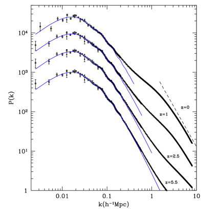
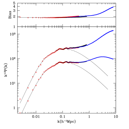
Figure 1 shows the evolution of the power spectrum of dark matter fluctuations in BigMDPL (circles), MDPL (triangles) and BolshoiP (squares) simulations. There is a remarkably good agreement between the simulations in overlapping regions. The plot also demonstrates with nice clarity the three dynamical regimes of growth of fluctuations: linear, quasi-linear with growth rates faster than linear and stable clustering with rates slower than quasi-linear. The power spectra and bias for dark matter halos and subhalos at redshift are shown in Figure 2. By plotting the power spectrum multiplied by we can see better the Baryonic Acoustic Oscillations (BAO).
The mass functions of halos at different redshifts in the Planck cosmology are shown in Figure 3. The Tinker et al. (2008) mass function provides an excellent fit to results and slightly underestimates the mass function at high redshifts. The differential mass function shows that the convergence of halo mass in the simulations is of the order of a few per cent. Compared to the suite of simulations, the prediction of Tinker et al. (2008) which was gauged at different cosmologies over-predicts the number of halos by less than 4% for halos below . (For definiteness we employed a quadratic interpolation to get the parameters for : )

3 Relaxed halos
Some dark matter halos may experience significant merging or strong interactions with environment that distort their density and kinematics, and hence, may bias the estimation of halo concentrations. To avoid possible biases due to non-equilibrium effects, we select and separately study halos that are expected to be close to equilibrium. Because halos grow in mass and have satellites moving inside them, there are no truly relaxed halos. However, by applying different selection conditions, we can select halos that are less affected by recent mergers and are closer to equilibrium.
A number of diagnostics have been used to select relaxed halos. These include the virial parameter , where and are the kinetic and potential energies, the offset parameter (distance between halo center and the center of mass), and the spin parameter (e.g. Neto et al., 2007; Macciò et al., 2007, 2008; Prada et al., 2012).
In addition to these three diagnostics, Neto et al. (2007) and Ludlow et al. (2012); Ludlow et al. (2014) also require that the fraction of mass in subhalos should be small, i.e. . This seems to be a reasonable condition, but we decided not to use it for two reasons. First, it is redundant: a combination of cuts in and already remove the vast majority of cases with . Figure 2 in Neto et al. (2007) clearly shows this. Second, this condition is very sensitive to resolution. Concentrations are often measured for halos with few thousand particles. For these halos one can reliably measure the spin and offset parameters, but detection of many subhalos is nearly impossible.
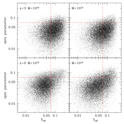
Figure 4 shows the distribution of spin and offset parameters for halos in the MDPL simulation at different redshifts and different masses. Note that the distribution of spin parameters is nearly independent of mass and redshift, a well known fact. Unlike the spin parameter, the distribution of visibly evolves with time. Dashed lines in the plot show our condition for relaxed halos:
| (6) |
Depending on redshift and mass, these conditions could select as “relaxed” most (% for halos at ) or small (% for halos at ) halo population.
In addition to the and diagnostics we also use the virial parameter . If halos are relaxed and isolated, then this parameter should be close to zero. Right panels in Figure 5 show the results for halos in the MDPL simulation at and .
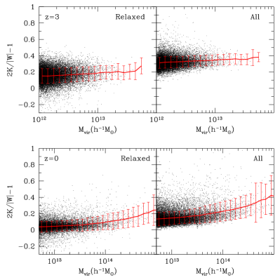

As it has been known for a long time that even the average virial parameter for a population of halos is not zero (e.g., Jang-Condell & Hernquist, 2001; Shaw et al., 2006; Neto et al., 2007). Results show that the kinetic energy is too large for halos to be in equilibrium. However, the conclusion that even at most of halos are significantly out of equilibrium is not correct. This is related with too simplistic application of the virial relation. Because halos are not isolated, a number of corrections must be taken into account to assess how far from the equilibrium they really are (Shaw et al., 2006; Knebe & Power, 2008; Davis et al., 2011; Power et al., 2012). Here we follow Davis et al. (2011), who presented the virial relation including effects of the surface pressure and external force. For a given halo with mass , radius , and kinetic energy , the virial equation should be written in the following form:
| (7) |
where the contribution of the external forces to the potential energy and the surface pressure term are:
| (8) | |||||
| (9) | |||||
| (10) |
Here the surface integral in the term is taken over the surface of a sphere of virial radius , and and are the density and radial velocity dispersion at .
We did not try to estimate the correction due to external forces, though simple estimates indicate that for low concentration halos it should be similar to . In order to estimate we use the halo profiles and find both the density and the radial velocity dispersion at the virial radius. We then estimate the term using eq. (10) and correct the virial parameter accordingly.
Left panels in Figure 5 and more detailed Figure 6 show effects of surface pressure correction as well as other corrections on the virial ratio . Typical value of the surface pressure correction is , which is similar to those found by Shaw et al. (2006); Knebe & Power (2008) and Davis et al. (2011). However, the correction depends on mass and on redshift. For the most massive halos at the correction is . It increases to for the most massive halos at .
Corrected values of the virial parameter are significantly closer to zero. For example, halos at with mass are very close to equilibrium, which is a dramatic improvement considering that all of them were considered to be out of equilibrium without the surface pressure correction. Just as Davis et al. (2011), we also find that the surface pressure correction, though an improvement, is not sufficient to bring the most massive and high- halos to equilibrium. Other corrections such as external forces and non-spherical effects are expected to bring those halos even closer to equilibrium. Unfortunately, it is difficult to estimate those.
Due to the uncertainty of the estimates of the virial parameter , one can apply somewhat loose conditions to select relaxed halos. For example, following Neto et al. (2007) and Ludlow et al. (2014), we may have used . The results in the right panels of Figure 5 show that this could have been a reasonable choice for halos, but not for high redshifts. For example, at , the vast majority of halos would be considered “unrelaxed” in spite of the fact that they are relaxed (i.e., pass the condition) once the surface pressure correction is applied.
The combination of a strict criterion for the virial parameter and the lack of correction for the surface pressure produces an unwanted side effect in results of Ludlow et al. (2012); Ludlow et al. (2014). Instead of selecting more relaxed halos, which was their intention, it results in selection of a biased sample of halos with unusually low concentrations and infall velocities.
Instead of applying the surface pressure correction and considering the fact that most of severely out-of-equilibrium halos are rejected by the offset and spin parameters, we adopt the selection applied to the uncorrected virial parameters.
4 Defining and measuring halo concentrations and density profiles

Dark matter halo density profiles are often approximated by the NFW profile (Navarro et al., 1997):
| (11) |
However, halo profiles can substantially deviate from the NFW shape and are much better approximated with an Einasto profile (Einasto, 1965; Navarro et al., 2004; Gao et al., 2008; Dutton & Macciò, 2014):
| (12) |
Here, the radius is the characteristic radius of the halo where the logarithmic slope of the density profile is equal to -2. It is often perceived that the Einasto profile provides accurate fits to the data because it has more free parameters: three instead of two for NFW. This conclusion is not correct. Even if the third parameter is fixed (defined by halo mass), the Einasto profile provides a better fit to simulation results (Gao et al., 2008). Nevertheless, there is a reason why the NFW profile was used for so long and why it is still a useful approximation.

The deviations of the NFW profile from -body results are small for halos that are not massive. For these halos the NFW and Einasto profiles are very close for a large range of radii . This point is illustrated in Figure 7 that gives examples of the circular velocity profiles for NFW and Einasto profiles. It shows the profiles for halos with the same virial mass and with the same characteristic radius , which was in this case chosen to be . To relate to we use eq. (13). The Einasto profiles with small parameters that are typical for halos with peak height , provide reasonable (though not perfect) approximations to the NFW with deviations for radii in the range (e.g., Ludlow et al., 2012). The situation is different for much more massive halos, which are larger peaks of the density field. For , the deviations are substantial even for radii where the circular velocity corresponding to the NFW profile is % below the Einasto profile (see also Gao et al., 2008).
The accuracy of the NFW approximation depends on parameters such as halo mass and redshift (e.g., Navarro et al., 2004). Gao et al. (2008) and Dutton & Macciò (2014) argue that the second parameter in the Einasto profile depends only on the amplitude of perturbations , where is the halo mass. Gao et al. (2008) provide the following approximation for the dependence of on the amplitude of perturbations:
| (13) |
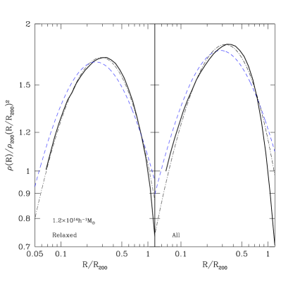
The observed large deviations from the NFW profile for high- peaks pose a number of problems for the estimates of halo concentrations because the concentrations are routinely estimated using NFW fits (e.g., Neto et al., 2007; Duffy et al., 2008; Diemer & Kravtsov, 2014a; Dutton & Macciò, 2014). Figure 8 shows an example that highlights the problem. At we select halos with mass in the BigMDPL simulation. These halos correspond to high density peaks of . We then construct the median halo density profiles for these halos and present them in Figure 8 for all and for relaxed halos. The plots demonstrate that the Einasto approximation provides remarkably accurate fits for the measured profiles with deviations less than 1% for the relaxed halos. The NFW profile is much less accurate. However, the real problem with the NFW fits is the systematic errors, not the random errors. The NFW fits systematically overpredict the halo concentration by (10–20)% for the high- halo density profiles shown in Figure 8. This and other systematic effects were recently discussed by Meneghetti & Rasia (2013) and Dutton & Macciò (2014).
One may think that using the Einasto profiles to estimate concentrations would produce much better results. Unfortunately, the Einasto profile has its own critical issue when it comes to concentration. For the NFW profile the ratio uniquely defines the density profile for given halo mass, and therefore it is a good measure for halo concentration. Yet, for the Einasto profile such a ratio is not the concentration because for the same ratio, halos with larger are clearly denser, and thus are more concentrated. In order to understand why is that, we need to step away from the problem of fitting profiles of cosmological dark matter halos and discuss what is concentration.
The common-sense notion of concentration is that for two objects of fixed mass and radius, the object with a more dense center is more concentrated. If we consider an astronomical quasi-spherical object such as a globular cluster, an elliptical galaxy, or a dark matter halo, then a more concentrated object is the one that has denser central region and less dense outer halo. Keeping in mind this general notion of concentration, we now look again at the NFW and Einasto profiles presented in Figure 7. All the profiles in the plot have the same virial mass, virial radius and . However, they all have different concentrations because they have different masses inside the central radius. This happens because the “shape parameter” in the Einasto profile affects not only the shape of the profile, but also its concentration.


Figure 9 illustrates the point. Here we analyze two Einasto profiles with the same total mass and the same ratio . The only difference is the shape parameter: and . For these density profiles Figure 9 shows two conventional measures of concentration: radius of a given fraction of mass (bottom panel) and fraction of mass within given radius (top panel). On all accounts, the profile with larger is more concentrated. For example, the radius of (1/3) of the virial mass is about 30% smaller for the model.
To summarize, for the Einasto profile the ratio is not the concentration. The real concentration depends on both and .
Following Prada et al. (2012) we use the ratio of the maximum circular velocity to the virial velocity as a profile-independent measure of halo concentration. The larger is the ratio, the larger is the halo concentration regardless of any particular analytical approximation of the profile.
It is convenient to write the circular velocity profile for the NFW and Einasto approximations in the following way:
| (14) | |||||
| (15) | |||||
| (16) | |||||
| (17) |
Here, functions and define the mass profiles for NFW and Einasto approximations correspondingly, and and are formal halo concentrations. Using these relations one can find the radius at the maximum of the circular velocity, .
Once ratio is measured in simulations, it can be used to estimate the formal concentration . For the Einasto approximation one can use one of the two relations in eq. (14):
| (19) | |||||
And for the NFW profile:
| (20) |

It is convenient to cast the ratio into the concentration using the NFW profile. For this we use eq. (20) to convert the velocity ratio into concentration . For halos that can be approximated by the NFW profile – and vast majority of them are – this gives us the familiar relation . For high- halos that are not approximated by the NFW profile, this still gives a measure of concentration: the larger the more dense is the central region of these halos. Because the mapping from the ratio to the concentration is monotonic, it always can be inverted to recover and then to find for halo with given parameter .
The BDM halofinder provides measurements of and for each halo, which are converted to estimates of concentration . When studying dependence of concentration on mass or , we bin halos according to their mass or . Halos in each bin (typically many thousands) are ranked by their values of and median values and deviations from the mean are found.
Similar procedure is used for dark matter profiles or profiles of the radial infall velocities and velocity anisotropy parameter . We normalize radii to the virial radius of each halo. Then profiles are binned using constant bin size in logarithm of radius . Radii are binned from % of to . For each radial bin, values from individual halos are ranked from the smallest to the largest and medians and deviations are found.
5 Halo profiles at different redshifts
Some of the halos in our simulations are resolved with millions of particles, but a vast majority have just few thousands. For this paper our goal is to study these numerous halos that are resolved from modest radius to . Simulations provide us the density profiles and also profiles of velocity dispersions, velocity anisotropies and radial infall velocities. Because of the wealth of information, we cannot show all combinations of halo profiles. Instead, we show only representative results.
One of the interesting issues is the structure of high- halos and the upturn in halo concentrations. In order to avoid possible complications with on-going major-mergers, we start the analysis with density profiles of relaxed halos. We select halos in a narrow range of masses and normalize distances by the virial radius and normalize densities by the density at the virial radius. Even with the narrow mass bins the number of halos in each bin is so large that the statistical errors of median values are very small. This is the reason why we do not show any statistical error bars in our plots.
The right panel Figure 10 shows density profiles for relaxed halos at . Even without fitting profiles with either NFW or Einasto profiles, the figure shows the well known trend with mass: more massive halos are less concentrated than the less massive ones. This can be seen by comparing densities at, say . There is another trend: the radius at which the density declines as (radius where curves in the plot are horizontal) increases with increasing mass. While the halos in the plot have large mass, in the sense of peak height they are not large: .
Halos at larger redshifts demonstrate strikingly different profiles. The left panel in Figure 10 presents halos at . Here the trend with mass is very different with more massive halos being more concentrated. There is a number of ways to demonstrate this. For example, inside a given fraction of virial radius larger halos have larger fraction of halo mass. Also the radius containing a given fraction of mass (another measure of concentration) is smaller for more massive halos. Another change in the halo profiles is the radius with the log-log slope -2 for density profiles. For these halos there is very little dependence of on halo mass.
Note that the halos at shown in the left panel of Figure 10 represent very large density peaks: . Indeed, it is mostly the height of the peak that defines the change in the structure of halo profiles. As we will see later, there is a dependence with the redshift, but this appears to be a weaker factor shaping the the structure of halos with peak height being the dominant effect. We can demonstrate this by selecting halos at the same redshift but with different .

For that we select relaxed halos at . The first sample of halos has mass and . These halos are in the regime of declining concentration-mass relation . Halos in the regime of the flat part of the are represented by halos with and and the upturn of the is represented by and . Profiles of these three types of halos are shown in Figure 11. Halos in the plateau of the have the lowest concentration and halos in the declining and upturn regimes are more concentrated. There is also a change in the shape of the density profiles. For example, the curves are broader for plateau halos and are more narrow for the upturn halos.

Figure 11 also shows rms deviations from the median profiles of halos. There is not much difference between different populations of halos. In this respect rare halos at the upturn are not more violent and do not have larger spread of densities as compared with “normal” halos of the declining population. However, many other halo properties do depend on .
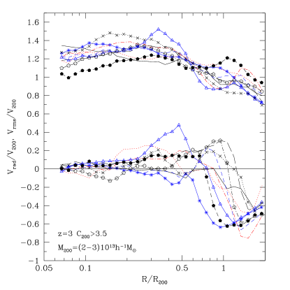
We start our analysis of velocity profiles of halos by presenting examples of radial and rms velocites of high peaks halos. Figure 12 presents velocity profiles (both radial and total rms) for all 10 halos in the simulation SMDPL at redshift with masses and concentrations . The halos are at the upturn. They clearly show strong infall velocities in the outer regions. However, the central regions, that define halo concentrtion, are quiet and have small radial velocities. Another indicator of relaxation is a large ratio of random velocites to the bulk radial velocities.
The average radial velocity profiles and the velocity anisotropy parameters are shown in Figures 13 and 14 for halos with different peak heights . Nearly zero average infall velocities indicate that central regions of halos are close to equilibrium at all times. This is true even for halos that are at the upturn regime of the relation. This confirms our estimates of the virial parameter in Sec. 3: corrected for the surface pressure the virial parameter is close to zero.
Negative values at radii larger than the virial radius indicate that matter falls into the halos resulting in its mass growth. However, the magnitude of the infalling velocities drastically depends on . It is nearly a half of the circular velocity at the virial radius for and goes to almost zero for (Prada et al., 2006; Cuesta et al., 2008; Diemer et al., 2013). Large infall velocities on high- halos are accompanied by very radial velocity anisotropy as demonstrated by right panels in Figure 14.
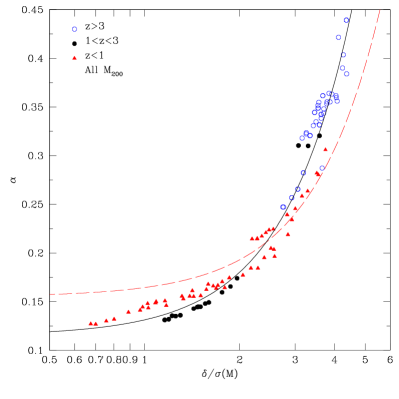
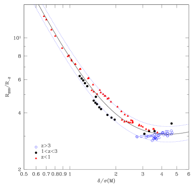
In order to characterize the density profiles of halos at different redshifts, masses and different , we stack profiles of halos binned by mass and normalize radii by virial radius of each halo. The number of halos in each mass bin is many hundreds and often thousands. We use only halos with more than 5000 particles. We then fit the Einasto profile eq.(12) using two free parameters: and . The third parameter is fixed to produce the total mass corresponding to the mass of selected halos. We note that this is not what is usually done (e.g., Macciò et al., 2007; Gao et al., 2008; Dutton & Macciò, 2014). Usually all three parameters are considered as free. This cannot be correct once the total mass is fixed by selecting halos by mass.
Parameters and of all halos in the Planck cosmology simulations SMDPL, MDPL, and bigMDPL are presented in Figure 15. Dependence of and on the peak height can be approximated with the following expressions:
| (21) | |||||
| (22) |
For relaxed halos we find that parameter is slightly smaller for high- halos and can be approximated as:
| (23) |
Evolution of halo density profiles for few halos around are given in Appendix B.
6 Halo Concentrations: evolution with redshift
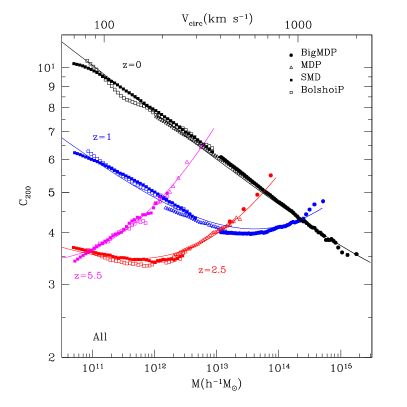
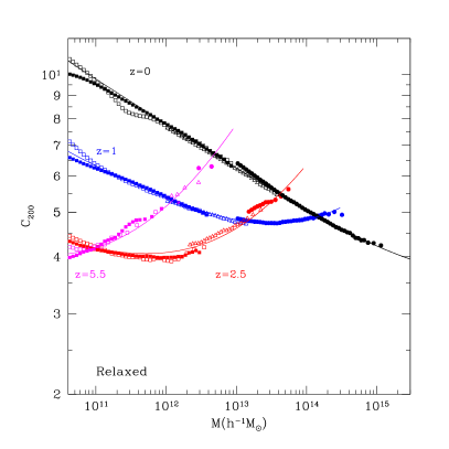
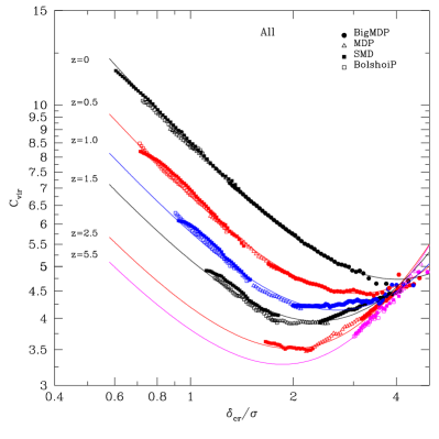
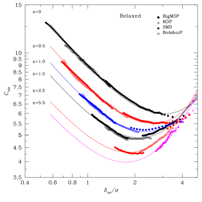
In addition to cosmological parameters, redshift, mass, and definition of virial radius, the halo concentration depends on how halos are selected. There are a number of options to do that. One can select all halos or only relaxed halos. Halos can be selected by virial mass or by circular velocity. Not surprisingly, different selection options result in a large number of combinations of approximations. However, qualitatively the results are the same. Figure 16 gives two examples of for halos selected in different ways. Here, we show the evolution of halo concentration defined using eq. (19) for halos selected by and by . The plots illustrate a well known result that the evolution of is quite complex (e.g. Prada et al., 2012). Nevertheless, qualitatively the pattern of the evolution is the same regardless how halos are selected.
The plots in Figure 16 show that there are three regimes for : a declining part on small masses, an upturn at very large masses and a plateau in between. Curves for and clearly illustrate this behavior. There is no declining part of at very large redshifts because our simulations do not have enough resolution to probe the declining brunch of .
As discussed in the previous section, the upturn in the concentration is related with the increase of at large masses. This is different for halos in the declining regime where the concentration declines mostly due to the change in the core radius while stays nearly constant.
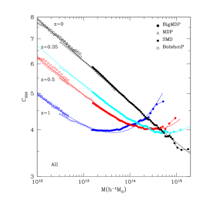
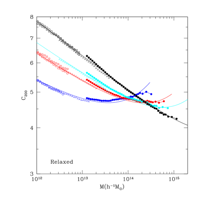
There is no upturn at . In order to shed light on this, we explore the evolution of halo concentration at low redshifts. Figure 17 shows that the concentration on the plateau starts to decline at and the upturn gets smaller and disappears at . Though the reason is not exactly clear, we speculate that this likely is related with the decline in matter density and, consequently, slower mass accretion on halos.
| Parameter | |||
|---|---|---|---|
| Redshift | |||
| 0.00 | 7.40 | 0.120 | |
| 0.35 | 6.25 | 0.117 | |
| 0.50 | 5.65 | 0.115 | |
| 1.00 | 4.30 | 0.110 | |
| 1.44 | 3.53 | 0.095 | |
| 2.15 | 2.70 | 0.085 | |
| 2.50 | 2.42 | 0.080 | |
| 2.90 | 2.20 | 0.080 | |
| 4.10 | 1.92 | 0.080 | |
| 5.40 | 1.65 | 0.080 | |
It is often convenient to have simple fits for concentration as function of mass for some redshifts. To make those fits we use the following 3-parameter functional form:
| (24) |
Table 2 gives parameters and for this approximation for the Planck cosmology. Parameters for additional selection conditions and for WMAP7 cosmology are presented in the Appendix A in tables 3– 8.
Following Prada et al. (2012) we study the evolution of halo concentrations as function of the amplitude of perturbations or as function of peak height . Evolution of the relation for halos defined using the virial mass and radius is presented in Figure 18 for the Planck cosmology for all and relaxed halos. As Figure 18 shows, the evolution of looks more simple as compared with . As Prada et al. (2012) and Diemer & Kravtsov (2014b) found, the shape of is almost the same at every redshift, but its position in the diagram gradually shifts. Here we find that the following functional form describes the shape of :
| (25) |
7 Upturn of halo concentration
The upturn in the concentration – mass relation is probably the most controversial regime. It was first discovered in Klypin et al. (2011) in the Bolshoi simulation made with the ART code. It later was found in the Millennium GADGET simulations and in the ART Multidark simulation by Prada et al. (2012) who made extensive analysis of halos at the upturn.
Considering that the upturn is a relatively new feature, some explanations were proposed. Ludlow et al. (2012) argue that the upturn is an artifact of halos that are out of equilibrium. Their idea can be summarized as follows. The most massive halos grow fast. When those halos are caught in the process of first major merger, the infalling satellite penetrates deep into the major halo producing an illusion of a very concentrated halo. When Ludlow et al. (2012) removed halos, which they perceived to be unrelaxed, they find that there is no upturn. The problem with this idea is that Ludlow et al. (2012) did not make the pressure term correction to the virial ratio. This renders most of the most massive halos to be considered unrelaxed when they actually are. The lack of infalling (radial) velocities in the central region of of the virial radius is also not consistent with the idea of “first infall” as an explanation for the upturn. So, the non-equilibrium explanation for the upturn does not seem to be valid.
Another idea for the upturn is related with the fact that in Klypin et al. (2011) and Prada et al. (2012) the concentration was estimated using the ratio. So, one may speculate that the upturn is due to the procedure. However, Prada et al. (2012) and more recently Dutton & Macciò (2014) compare estimates of concentration done with fitting the NFW profiles and with the ratio. They find that both methods produce nearly identical results for most of halos. Systematic 10% differences in concentration were found only for the most massive halos. However, the problem with the fitting densities of the massive halos is that the profiles substantially deviate from the NFW profile. For these halos only the ratio was reported as a concentration, thus missing the main contribution to the concentration, i.e. the increase of .
The properties of halos at the upturn point into a different explanation for the origin of the upturn. These extremely massive halos form around very high density peaks of initial linear density perturbations. The analysis of statistical properties of gaussian random fields shows that these rare peaks tend to be more spherical than low- peaks (Doroshkevich, 1970; Bardeen et al., 1986). In turn, this means that infall velocities are also more radial resulting in deeper penetration of infalling mass into the halo. This produces more centrally concentrated halos.
This large concentration will not be preserved as more material is accreted. As the mass grows, the relative peak height becomes lower and the infall velocities become less radial. The halo gradually slides into the plateau regime. As the rate of accretion decreases even more, the central region stops to be severely affected by mergers, which now tend to build more extended outer regions. This will be the “normal” slow growth mode of halos and associated with the decline regime in the concentration – mass relation.
8 Comparison with other results
There are some differences between our results with those in Prada et al. (2012). We now have more data, which allow us to make more detailed analysis of concentrations. We also make fits of density profiles using the Einasto profiles. In Prada et al. (2012) we used only bound particles to estimate profiles and concentrations. Even for the most massive halos the average fraction of unbound particles is less than 3%. However, this increases the halo concentration by as much as %.
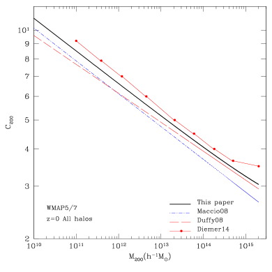
We start with comparing different published estimates of halo concentrations at redshift . In the left panel of Figure 19 we compare different published results of concentrations defined using the NFW profiles for all halos in the WMAP5/7 cosmologies. Overall, the agreement between different groups is quite reasonable, but there some systematic difference. For example, results of Duffy et al. (2008) and Macciò et al. (2008) are systematically below our estimates by %. Concentrations in Diemer & Kravtsov (2014a) are 5% above ours. They also find some indication of an upturn at the largest masses, which we do not see in our simulations.
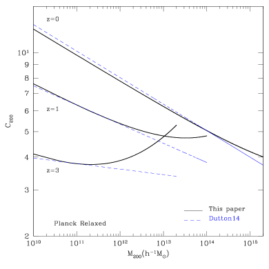
We compare concentrations for the Planck cosmology at different redshifts in the right panel of Figure 19. Here, we compare NFW-based concentrations for relaxed halos in our simulations with those in Dutton & Macciò (2014). There is an excellent agreement for with deviations less than 2%. The situation is more complicated at high redshifts with again very good agreement at low masses and substantial differences at large masses. However, one should remember that Dutton & Macciò (2014) fit the NFW profiles to the data and we do not. Because the most massive halos at high redshifts have large deviations from the NFW profiles, not surprisingly we have large differences between our estimates and those of Dutton & Macciò (2014).
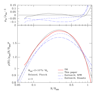
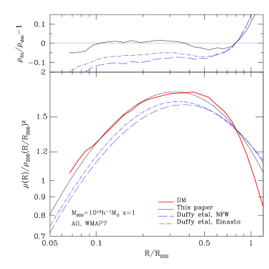
Because halo concentrations are used to estimate density profiles, it is important to compare different predictions for dark matter density profiles, not just concentrations. We give two examples of such a comparison. In the right panel of Figure 20 we show the median density profile of all halos at redshift with mass in the WMAP7 MultiDark simulation. The black thin curve also shows our approximation using the Einasto profile with parameters defined by eqs.(21-23). We also compare our results with the predictions given in Table 1 of Duffy et al. (2008) for both NFW and Einasto profiles. Those predictions are systematically below the results of simulations by %. Note that the problem cannot be fixed by scaling up the density profiles to improve the accuracy of the fits. This cannot be done because the total halo mass will be substantially larger than the mass of the halo in the simulation.
The failure of the Einasto fit in the Duffy et al. (2008) approximation is related to their approximation for the parameter. Duffy et al. (2008) used results from Gao et al. (2008) (eq. 13) that gives a 10% smaller value of as compared with our estimate given by eq. (21). Combined with a slightly smaller value of the formal concentration, this results in the halo density profile, which is systematically misses by 10% the density in the simulation.
Comparison of our density profiles with those by Dutton & Macciò (2014) shows much better agreement as indicated in the left panel of Figure 20 when the Einasto profile is used. Here, we show density profile for relaxed halos with in the Planck cosmology simulation MDPL at . The total of 300 halos where used to produce the median profile. Halos of this mass and redshift have , which puts them in the upturn of the concentration - mass relation. Our analytical fit for the density profile is obtained using eq. (23) for the parameter. The ratio is estimated using eq. (22), which we scale up by factor 1.1 to account for the fact that relaxed halos are more concentrated than all halos. To construct profiles predicted by Dutton & Macciò (2014), we use parameters for the NFW and Einasto approximations from their Table 3. All analytical fits are normalized to have the same total halo mass.
It is clear that the NFW fit given by Dutton & Macciò (2014) provides a halo, which is less concentrated than that in the simulation. This is consistent with the differences which we saw in the right panel of Figure 19: the NFW fits predict too low concentrations for halos at the upturn resulting in % too low densities. However, the differences between our and Dutton & Macciò (2014) Einasto fits are significantly smaller.
9 How to estimate density profiles
We offer different options to estimate density profiles of dark matter halos. Halos in the declining branch of the relation () can be approximated using the NFW profile. Tables in the Appendix A give numerous parameters for halos selected in different ways. One can interpolate between the values provided by the Tables to find the approximations for different redshifts. The interpolation of parameters is expected to be more accurate because there is less evolution of the parameters with the redshift.
There are two options for handling halos at the plateau and upturn. For all halos in the Planck cosmology one can use eqs.(21-22) to find and . For other selection conditions and for the WMAP cosmology, one should use eqs.(21) or eqs.(23) to find . These relations are expected to be least dependent on details of selection and cosmological parameters. Then one should use one of the approximations for given in the Appendix A. Finally, solve eqs.(19-20) to find for known and .
10 Conclusions
In this paper we present the new suite of MultiDark cosmological N-body simulations from which we have identified more than 60 billion dark matter halos with more than 100 particles that span more than 5 orders of magnitude in mass and covers more than 50 Gpc3 in volume. From this large data set we have studied with very high accuracy the halo density, infall velocity and velocity anisotropy profiles and concentrations in three dynamical regimes: declining concentration, plateau, and upturn. We derive analytical approximations that provide 2–5% accurate estimates for halo concentrations and density profiles.
We summarize the main results from this work:
-
•
In order to understand the evolution of halo concentration and, specifically the nature of the upturn, one needs to realize that the halo concentration is not defined as the ratio of the virial radius to the radius as in the NFW profile. For massive halos the average density profile is far from the NFW shape and the concentration is not defined by the core radius . In Section 5 we present density profiles that clearly show that massive halos at have increasing concentrations with increasing mass and they have nearly unchanging . Both parameters and of the Einasto approximation affect the concentration.
-
•
We speculate that the increase in the halo concentrations for the most massive halos is related with the tendency of rare peaks in the random gaussian linear density field to be more spherical (Doroshkevich, 1970; Bardeen et al., 1986). Very radial accretion onto these peaks is clearly seen in Figure 14 with the average velocity anisotropy parameter for halos with . This radial infall brings mass closer to the center, producing a highly concentrated halo. As time goes on the halo slides into the plateau regime, and accretion becomes less radial. Now mass is deposited at larger radius, and the concentration declines. Once the rate of accretion and merging slows down, the halo moves into the domain of declining because new accretion piles up mass close to the virial radius while the core radius is staying constant.
-
•
The ratio of the maximum circular velocity to the virial velocity gives a profile-independent measure of the halo concentration.
-
•
Density profiles of very massive halos with substantially deviate from the NFW shape. Fitting an NFW profile for these halos gives incorrect results regardless on how the fitting (what range of radii) is done. The differences between the NFW and Einasto concentrations for these massive halos do not mean that there are uncertainties in halo concentration. They simply indicate that the NFW formula should not be used.
-
•
Differences between the concentration and the formal concentration obtained by fitting the Einasto profile (the ratio ) do not indicate that there are real disagreements. These two estimates are for different quantities. The ratio is only a part of the real halo concentration.
Acknowledgements
The BigMultidark simulations have been performed on the SuperMUC supercomputer at the Leibniz-Rechenzentrum (LRZ) in Munich, using the computing resources awarded to the PRACE project number 2012060963. The SMDPL and HMDPL simulations have been performed on SuperMUC at LRZ in Munich within the pr87yi project. Bolshoi(P) and MultiDark simulations were performed on Pleiades supercomputer at the NASA Ames supercomputer center. S. H. wants to thank R. Wojtak for useful discussions. The authors want to thank V. Springel for providing us with the optimized version of GADGET-2. S.H. acknowledges support by the Deutsche Forschungsgemeinschaft under the grant . A.K. acknowledges support of NSF grants to NMSU. GY acknowledges support from MINECO (Spain) under research grants AYA2012-31101 and FPA2012-34694 and Consolider Ingenio SyeC CSD2007-0050 FP acknowledge support from the Spanish MICINNs Consolider-Ingenio 2010 Programme under grant MultiDark CSD2009-00064, MINECO Centro de Excelencia Severo Ochoa Programme under grant SEV-2012-0249, and MINECO grant AYA2014-60641-C2-1-P
References
- Alimi et al. (2012) Alimi J.-M. et al., 2012, ArXiv e-prints 1206.2838
- Angulo et al. (2012) Angulo R. E., Springel V., White S. D. M., Jenkins A., Baugh C. M., Frenk C. S., 2012, MNRAS, 426, 2046
- Angulo & White (2010) Angulo R. E., White S. D. M., 2010, MNRAS, 405, 143
- Bardeen et al. (1986) Bardeen J. M., Bond J. R., Kaiser N., Szalay A. S., 1986, ApJ, 304, 15
- Behroozi et al. (2013) Behroozi P. S., Wechsler R. H., Wu H.-Y., 2013, ApJ, 762, 109
- Bryan & Norman (1998) Bryan G. L., Norman M. L., 1998, ApJ, 495, 80
- Bullock et al. (2001) Bullock J. S., Kolatt T. S., Sigad Y., Somerville R. S., Kravtsov A. V., Klypin A. A., Primack J. R., Dekel A., 2001, MNRAS, 321, 559
- Crocce et al. (2010) Crocce M., Fosalba P., Castander F. J., Gaztañaga E., 2010, MNRAS, 403, 1353
- Cuesta et al. (2008) Cuesta A. J., Prada F., Klypin A., Moles M., 2008, MNRAS, 389, 385
- Davis et al. (2011) Davis A. J., D’Aloisio A., Natarajan P., 2011, MNRAS, 416, 242
- Diemer & Kravtsov (2014a) Diemer B., Kravtsov A. V., 2014a, ArXiv e-prints
- Diemer & Kravtsov (2014b) Diemer B., Kravtsov A. V., 2014b, ArXiv e-prints
- Diemer et al. (2013) Diemer B., More S., Kravtsov A. V., 2013, ApJ, 766, 25
- Doroshkevich (1970) Doroshkevich A. G., 1970, Astrophysics, 6, 320
- Duffy et al. (2008) Duffy A. R., Schaye J., Kay S. T., Dalla Vecchia C., 2008, MNRAS, 390, L64
- Dutton & Macciò (2014) Dutton A. A., Macciò A. V., 2014, MNRAS, 441, 3359
- Einasto (1965) Einasto J., 1965, Trudy Astrofizicheskogo Instituta Alma-Ata, 5, 87
- Gao et al. (2008) Gao L., Navarro J. F., Cole S., Frenk C. S., White S. D. M., Springel V., Jenkins A., Neto A. F., 2008, MNRAS, 387, 536
- Gottloeber & Klypin (2008) Gottloeber S., Klypin A., 2008, ArXiv e-prints
- Jang-Condell & Hernquist (2001) Jang-Condell H., Hernquist L., 2001, ApJ, 548, 68
- Jing (2000) Jing Y. P., 2000, ApJ, 535, 30
- Kim et al. (2009) Kim J., Park C., Gott III J. R., Dubinski J., 2009, ApJ, 701, 1547
- Klypin & Holtzman (1997) Klypin A., Holtzman J., 1997, ArXiv Astrophysics e-prints
- Klypin et al. (2011) Klypin A. A., Trujillo-Gomez S., Primack J., 2011, ApJ, 740, 102
- Knebe et al. (2011) Knebe A. et al., 2011, MNRAS, 415, 2293
- Knebe & Power (2008) Knebe A., Power C., 2008, ApJ, 678, 621
- Kravtsov et al. (1997) Kravtsov A. V., Klypin A. A., Khokhlov A. M., 1997, Rev.Astrn.Astrophys., 111, 73
- Ludlow et al. (2014) Ludlow A. D., Navarro J. F., Angulo R. E., Boylan-Kolchin M., Springel V., Frenk C., White S. D. M., 2014, MNRAS, 441, 378
- Ludlow et al. (2013) Ludlow A. D. et al., 2013, MNRAS, 432, 1103
- Ludlow et al. (2012) Ludlow A. D., Navarro J. F., Li M., Angulo R. E., Boylan-Kolchin M., Bett P. E., 2012, MNRAS, 427, 1322
- Macciò et al. (2008) Macciò A. V., Dutton A. A., van den Bosch F. C., 2008, MNRAS, 391, 1940
- Macciò et al. (2007) Macciò A. V., Dutton A. A., van den Bosch F. C., Moore B., Potter D., Stadel J., 2007, MNRAS, 378, 55
- Meneghetti & Rasia (2013) Meneghetti M., Rasia E., 2013, ArXiv e-prints
- Navarro et al. (1997) Navarro J. F., Frenk C. S., White S. D. M., 1997, ApJ, 490, 493
- Navarro et al. (2004) Navarro J. F. et al., 2004, MNRAS, 349, 1039
- Neto et al. (2007) Neto A. F. et al., 2007, MNRAS, 381, 1450
- Nuza et al. (2013) Nuza S. E. et al., 2013, MNRAS, 432, 743
- Power et al. (2012) Power C., Knebe A., Knollmann S. R., 2012, MNRAS, 419, 1576
- Prada et al. (2012) Prada F., Klypin A. A., Cuesta A. J., Betancort-Rijo J. E., Primack J., 2012, MNRAS, 423, 3018
- Prada et al. (2006) Prada F., Klypin A. A., Simonneau E., Betancort-Rijo J., Patiri S., Gottlöber S., Sanchez-Conde M. A., 2006, ApJ, 645, 1001
- Riebe et al. (2013) Riebe K. et al., 2013, Astronomische Nachrichten, 334, 691
- Shaw et al. (2006) Shaw L. D., Weller J., Ostriker J. P., Bode P., 2006, ApJ, 646, 815
- Springel (2005) Springel V., 2005, MNRAS, 364, 1105
- Teyssier et al. (2009) Teyssier R. et al., 2009, Astr.Astrophy., 497, 335
- Tinker et al. (2008) Tinker J., Kravtsov A. V., Klypin A., Abazajian K., Warren M., Yepes G., Gottlöber S., Holz D. E., 2008, ApJ, 688, 709
- van den Bosch (2002) van den Bosch F. C., 2002, MNRAS, 331, 98
- Watson et al. (2013) Watson W. A., Iliev I. T., Diego J. M., Gottlöber S., Knebe A., Martínez-González E., Yepes G., 2013, ArXiv e-prints
- Wechsler et al. (2002) Wechsler R. H., Bullock J. S., Primack J. R., Kravtsov A. V., Dekel A., 2002, ApJ, 568, 52
- Zhao et al. (2009) Zhao D. H., Jing Y. P., Mo H. J., Börner G., 2009, ApJ, 707, 354
- Zhao et al. (2003) Zhao D. H., Mo H. J., Jing Y. P., Börner G., 2003, MNRAS, 339, 12
Appendix A Parameters for the concentration - mass relation
Tables 3 – 10 give parameters for approximation eq.(24) for different simulations, virial mass definitions, halo selection criteria, and redshifts.
| Parameter | |||
| Redshift | |||
| Relaxed halos selected by mass | |||
| 0.00 | 7.75 | 0.100 | |
| 0.35 | 6.70 | 0.095 | |
| 0.50 | 6.25 | 0.092 | |
| 1.00 | 5.02 | 0.088 | |
| 1.44 | 4.19 | 0.085 | |
| 2.15 | 3.30 | 0.083 | |
| 2.50 | 3.00 | 0.080 | |
| 2.90 | 2.72 | 0.080 | |
| 4.10 | 2.40 | 0.080 | |
| 5.40 | 2.10 | 0.080 | |
| All halos selected by mass | |||
| 0.00 | 7.40 | 0.120 | |
| 0.35 | 6.25 | 0.117 | |
| 0.50 | 5.65 | 0.115 | |
| 1.00 | 4.30 | 0.110 | |
| 1.44 | 3.53 | 0.095 | |
| 2.15 | 2.70 | 0.085 | |
| 2.50 | 2.42 | 0.080 | |
| 2.90 | 2.20 | 0.080 | |
| 4.10 | 1.92 | 0.080 | |
| 5.40 | 1.65 | 0.080 | |
| Parameter | |||
| Redshift | |||
| Relaxed halos selected by | |||
| 0.00 | 8.0 | 0.100 | |
| 0.35 | 6.82 | 0.095 | |
| 0.50 | 6.40 | 0.092 | |
| 1.00 | 5.20 | 0.088 | |
| 1.44 | 4.35 | 0.085 | |
| 2.15 | 3.50 | 0.080 | |
| 2.50 | 3.12 | 0.080 | |
| 2.90 | 2.85 | 0.080 | |
| 4.10 | 2.55 | 0.080 | |
| 5.40 | 2.16 | 0.080 | |
| All halos selected by | |||
| 0.00 | 7.75 | 0.115 | |
| 0.35 | 6.50 | 0.115 | |
| 0.50 | 5.95 | 0.115 | |
| 1.00 | 4.55 | 0.110 | |
| 1.44 | 3.68 | 0.105 | |
| 2.15 | 2.75 | 0.100 | |
| 2.50 | 2.50 | 0.095 | |
| 2.90 | 2.25 | 0.090 | |
| 4.10 | 2.05 | 0.080 | |
| 5.40 | 1.76 | 0.080 | |
| Parameter | |||
| Redshift | |||
| Relaxed halos selected by mass | |||
| 0.00 | 10.2 | 0.100 | |
| 0.35 | 7.85 | 0.095 | |
| 0.50 | 7.16 | 0.092 | |
| 1.00 | 5.45 | 0.088 | |
| 1.44 | 4.55 | 0.085 | |
| 2.15 | 3.55 | 0.080 | |
| 2.50 | 3.24 | 0.080 | |
| 2.90 | 2.92 | 0.080 | |
| 4.10 | 2.60 | 0.080 | |
| 5.40 | 2.30 | 0.080 | |
| All halos selected by mass | |||
| 0.00 | 9.75 | 0.110 | |
| 0.35 | 7.25 | 0.107 | |
| 0.50 | 6.50 | 0.105 | |
| 1.00 | 4.75 | 0.100 | |
| 1.44 | 3.80 | 0.095 | |
| 2.15 | 3.00 | 0.085 | |
| 2.50 | 2.65 | 0.080 | |
| 2.90 | 2.42 | 0.080 | |
| 4.10 | 2.10 | 0.080 | |
| 5.40 | 1.86 | 0.080 | |
| Parameter | |||
| Redshift | |||
| Relaxed halos selected by | |||
| 0.00 | 10.7 | 0.110 | |
| 0.35 | 8.1 | 0.100 | |
| 0.50 | 7.33 | 0.100 | |
| 1.00 | 5.65 | 0.088 | |
| 1.44 | 4.65 | 0.085 | |
| 2.15 | 3.70 | 0.080 | |
| 2.50 | 2.35 | 0.080 | |
| 2.90 | 2.98 | 0.080 | |
| 4.10 | 2.70 | 0.080 | |
| 5.40 | 2.35 | 0.080 | |
| All halos selected by | |||
| 0.00 | 10.3 | 0.115 | |
| 0.35 | 7.6 | 0.115 | |
| 0.50 | 6.83 | 0.115 | |
| 1.00 | 4.96 | 0.110 | |
| 1.44 | 3.96 | 0.105 | |
| 2.15 | 3.00 | 0.100 | |
| 2.50 | 2.73 | 0.095 | |
| 2.90 | 2.45 | 0.090 | |
| 4.10 | 2.24 | 0.080 | |
| 5.40 | 2.03 | 0.080 | |
| Parameter | |||
| Redshift | |||
| Relaxed halos selected by mass | |||
| 0.0 | 6.90 | 0.090 | |
| 0.50 | 5.70 | 0.088 | |
| 1.00 | 4.55 | 0.086 | |
| 1.44 | 3.75 | 0.085 | |
| 2.15 | 2.9 | 0.085 | |
| 2.50 | 2.6 | 0.085 | |
| 2.90 | 2.4 | 0.085 | |
| 4.10 | 2.2 | 0.085 | |
| All halos selected by mass | |||
| 0.0 | 6.60 | 0.110 | |
| 0.50 | 5.25 | 0.105 | |
| 1.00 | 3.85 | 0.103 | |
| 1.44 | 3.0 | 0.097 | |
| 2.15 | 2.1 | 0.095 | |
| 2.50 | 1.8 | 0.095 | |
| 2.90 | 1.6 | 0.095 | |
| 4.10 | 1.4 | 0.095 | |
| Relaxed halos selected by | |||
| 0.0 | 7.20 | 0.090 | |
| 0.50 | 5.90 | 0.088 | |
| 1.00 | 4.70 | 0.086 | |
| 1.44 | 3.85 | 0.085 | |
| 2.15 | 3.0 | 0.085 | |
| 2.50 | 2.7 | 0.085 | |
| 2.90 | 2.5 | 0.085 | |
| 4.10 | 2.3 | 0.085 | |
| Parameter | |||
| Redshift | |||
| Relaxed halos selected by mass | |||
| 0.0 | 9.50 | 0.090 | |
| 0.50 | 6.75 | 0.088 | |
| 1.00 | 5.00 | 0.086 | |
| 1.44 | 4.05 | 0.085 | |
| 2.15 | 3.10 | 0.085 | |
| 2.50 | 2.80 | 0.085 | |
| 2.90 | 2.45 | 0.085 | |
| 4.10 | 2.20 | 0.085 | |
| All halos selected by mass | |||
| 0.0 | 9.00 | 0.100 | |
| 0.50 | 6.00 | 0.100 | |
| 1.00 | 4.30 | 0.100 | |
| 1.44 | 3.30 | 0.100 | |
| 2.15 | 2.30 | 0.095 | |
| 2.50 | 2.10 | 0.095 | |
| 2.90 | 1.85 | 0.095 | |
| 4.10 | 1.70 | 0.095 | |
| Relaxed halos selected by | |||
| 0.0 | 9.75 | 0.085 | |
| 0.50 | 7.02 | 0.085 | |
| 1.00 | 5.23 | 0.085 | |
| 1.44 | 4.25 | 0.085 | |
| 2.15 | 3.20 | 0.085 | |
| 2.50 | 2.90 | 0.085 | |
| 2.90 | 2.50 | 0.085 | |
| 4.10 | 2.35 | 0.085 | |
| Parameter | ||
| Redshift | ||
| All halos selected by mass | ||
| 0.0 | 0.278 | 0.40 |
| 0.38 | 0.375 | 0.65 |
| 0.50 | 0.411 | 0.82 |
| 1.00 | 0.436 | 1.08 |
| 1.44 | 0.426 | 1.23 |
| 2.50 | 0.375 | 1.60 |
| 2.89 | 0.360 | 1.68 |
| 5.41 | 0.351 | 1.70 |
| Relaxed halos selected by mass | ||
| 0.0 | 0.522 | 0.95 |
| 0.38 | 0.550 | 1.06 |
| 0.50 | 0.562 | 1.15 |
| 1.00 | 0.562 | 1.28 |
| 1.44 | 0.541 | 1.39 |
| 2.50 | 0.480 | 1.66 |
| 2.89 | 0.464 | 1.70 |
| 5.41 | 0.450 | 1.72 |
| All halos selected by | ||
| 0.0 | 0.41 | 0.65 |
| 1.00 | 0.49 | 1.15 |
| 2.50 | 0.41 | 1.60 |
| Parameter | ||
| Redshift | ||
| All halos selected by mass | ||
| 0.0 | 0.567 | 0.75 |
| 0.38 | 0.541 | 0.90 |
| 0.50 | 0.529 | 0.97 |
| 1.00 | 0.496 | 1.12 |
| 1.44 | 0.474 | 1.28 |
| 2.50 | 0.421 | 1.52 |
| 5.50 | 0.393 | 1.62 |
| Relaxed halos selected by mass | ||
| 0.0 | 0.716 | 0.99 |
| 0.38 | 0.673 | 1.10 |
| 0.50 | 0.660 | 1.16 |
| 1.00 | 0.615 | 1.29 |
| 1.44 | 0.585 | 1.41 |
| 2.50 | 0.518 | 1.65 |
| 5.50 | 0.476 | 1.72 |
Appendix B Examples of evolution of halo concentration and mass accretion history.
In Sections 5 and 6 we discussed the evolution of the average properties of halos, including density profiles and halo concentrations. In this appendix we focus on a somewhat different but related issue: how individual halos evolve. The evolution of individual halos has been extensively studied over the past 15 years (e.g., Wechsler et al., 2002; van den Bosch, 2002; Zhao et al., 2009; Ludlow et al., 2013, 2014). Here we do not intent to make a comprehensive analysis of the individual halo assmbly tracks, but provide typical examples of how concentrations and some other basic properties of individual very large halos – as opposed to the average – evolve over time.
Our main focus is on halos that are located at the upturn or on the plateau of the concentration-mass relation. Being the most massive, these halos typically grow very fast at large redshifts. Does it mean, as it was argued by Ludlow et al. (2012), that these halos are substantially out of equilibrium?
For our analysis we use halo tracks selected in the BolshoiP simulation. Because we are interested in the evolution of very large halos, this simulation provides a compromise between mass resolution and halo statistics.
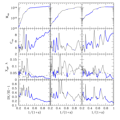
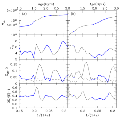
We start with presenting tracks of six halos that have at a mass of . The halos were selected to be relaxed at , but no other selection conditions were used. Figure 21 shows the evolution of different global parameters of these halos. Large variations in halo concentration are seen at high redshifts when halo mass increases very quickly. Once the mass accretion slows down at low redshifts, halo concentration shows the tendency to increase with time. This behavior is well known and has been well studied (e.g., Bullock et al., 2001; Wechsler et al., 2002).
There is also another trend with time: the virial ratio tends to decrease with time as the concentration increases. This is in line with the arguments put forward in Section 3. Indeed, as the concentration increases, the effects of the surface pressure become smaller, and the virial ratio also have a tendency to be smaller.
The three right panels in Figure 21 show examples of major mergers in the regime when the mass accretion slows down at low redshifts. For example, the first halo on the right experiences the merging event at (expansion parameter ). Just as the merging event proceeds, the halo concentration shows a sharp increase by climbing from , before the merger, to the peak value of . This happens when the infalling satellite reaches the center of halo, increasing the mass and, thus, halo concentration before bouncing back. This is definitely a sign of an out-of-equilibrium event. The jump in concentration disappears quickly after the onset of the merger. The same effect during major merger event was found by Ludlow et al. (2012). Most of the time, but not always, this jump in concentration is flagged as happening in a non-relaxed halo. This behavior of halo concentration is typical for halos at low redshifts (or at low peaks): rare major mergers result in jumps in mass followed by bumps in halo concentration.
The situation with mass accretion and concentration is more complicated in the case of fast growing high- halos. Halos in the left side of Figure 21 indicate that at , when halos quickly increase mass, their concentration experiences large fluctuations and overall do not grow with time.
In order to explore this domain of halo evolution in more detail, we focus on the most massive halos at . Specifically, we study large halos with at . The vast majority (%) of these halos more than double their mass in a dynamical time, which for these halos is typically equal to yrs. However, the crossing time of the central region, which defines the halo concentration, is significantly shorter: yrs, where is the core radius, and is the 3d rms velocity of dark matter particles in the central region. This short central time-scale allows the central halo region to quickly relax and adjust to ever infalling numerous satellites.
We can approximately split all halos at that redshift and mass range into “upturn” and “normal” halos by considering halos with to be in the upturn (see Figure 16). Overall, about 2/3 of all halos are in the upturn and 1/4 of all halos are relaxed upturn halos.
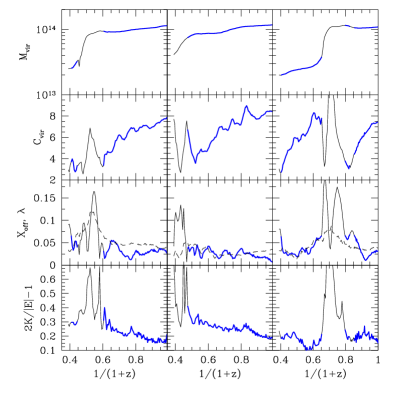
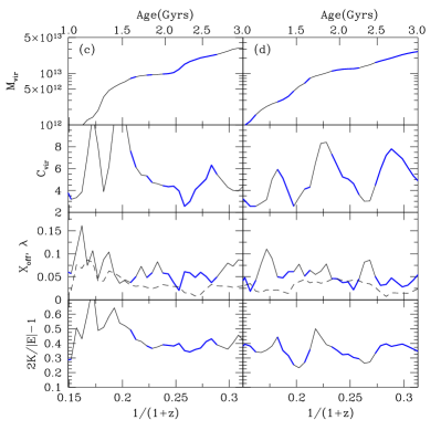
Figure 22 shows the evolution of four upturn halos. These halos were selected to be relaxed and have large concentration at . The mass accretion history of these halos shows occasional major merger events in their past, but there only few of theses events, and most of the mass accretion happens as a steady and fast mass growth, not major merger. This is also confirmed by studying masses and positions of largest subhalos. In all cases the most massive subhalo had just (1-3)% of the halo mass at . However, there are many of the subhalos and their total mass is substantial with the first 20 most massive subhalos providing (10-15)% of the total halo mass.
For example, halo (a) (left-most halo in Figure 22) has a major merger event at Gyrs, which was followed by a “normal” spike in its concentration. At ( Gyrs) it had large concentration that is clearly not related with the early major merger. Indeed, it does not show any large subhalo moving through its central region that would be responsible for the large concentration. Other halos in the figure do not have signatures of major mergers at Gyrs.
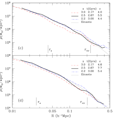
In left panels in figure 23 we show the evolution of halo profiles for two upturn halos presented in Figure 22. There are clear signs of large variations in the density at large radii comparable to the virial radius, and there are some variations in the central region too. However, the evolution of the density in the central region is better described as a gradual increase, not a sudden change that one may expect if the halo was drastically out of equilibrium.
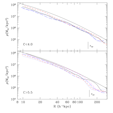
The right two panels shown in Figure 23 give examples of high concentration upturn halos (, bottom panel) and low concentration halos (, top panel). To guide the eye, the top dotted curve in each plot shows the same Einasto profile. High concentration halos are slightly denser and have larger fluctuations around the virial radius. They also have systematically different profile shapes with steeper decline in the outer regions. Still, there are no drastic differences between high and low concentration halos.
These results indicate that major mergers, though important and happening, do not explain the phenomenon of the upturn halos. What we find is more consistent with the picture where fast and preferentially radial infall of numerous satellites results in a quasi-equilibrium drift of the halo concentration. Because the infalling mass settles at different radii, the concentration does not increase with time but experiences large up-and-down variations.