Formation and properties of astrophysical carbonaceous dust. I: ab-initio calculations of the configuration and binding energies of small carbon clusters

Abstract

The binding energies of $n<100$ carbon clusters are calculated using the ab-initio density functional theory code Quantum Espresso. Carbon cluster geometries are determined using several levels of classical techniques and further refined using density functional theory. The resulting energies are used to compute the work of cluster formation and the nucleation rate in a saturated, hydrogen-poor carbon gas. Compared to classical calculations that adopt the capillary approximation, we find that nucleation of carbon clusters is enhanced at low temperatures and depressed at high temperatures. This difference is ascribed to the different behavior of the critical cluster size. We find that the critical cluster size is at $n=27$ or $n=8$ for a broad range of temperatures and saturations, instead of being a smooth function of such parameters. The results of our calculations can be used to follow carbonaceous cluster/grain formation, stability, and growth in hydrogen poor environments, such as the inner layers of core-collapse supernova and supernova remnants.

1 Introduction

Dust plays an important role at many levels in the observability, the dynamics, and the evolution of astrophysical phenomena. Many heavy atoms produced in stellar explosions are found in dust (Weingartner & Draine 2001). The formation of planetary and stellar systems is heavily affected by the abundance of dust (Whittet 2003); in particular dust is the the building block of rocky planets in protoplanetary disks (Blum & Wurm 2008). Furthermore, dust in the ISM scatters ultraviolet and visible light, and emits brightly in the infrared (Draine 2003).

However, dust formation in stellar and galactic environments is not well understood. The observation of crystalline silicates (Spoon et al. 2006; Speck et al. 2008) and dust formation in the hostile environment of colliding winds of WR stars (Williams et al. 1990; Varricatt et al. 2004) underline serious holes in our understanding of the physics of the phase transition at the base of dust formation. In addition, theoretical predictions of dust formation in supernova explosions over-predict the amount of dust observed at early times by several orders of magnitudes (on timescales of one year after core-collapse) (Todini & Ferrara 2001; Fallest et al. 2011; Gall et al. 2014). The limitations of the classical theory of nucleation for dust formation have been repeatedly pointed out (Donn & Nuth 1985; Jones 2001; Lazzati 2008; Cherchneff & Dwek 2009, 2010). Among the weaknesses of the theory is that of assuming quasi-equilibrium conditions for a strongly out of equilibrium phenomenon, the assumption of local thermal equilibrium, ignoring the presence of other components in the gas phase, and the capillary approximation. The capillary approximation is used to predict the binding energy of very small molecular clusters by assuming: (i) that they are spherical in shape, (ii) that a surface can be defined for them, and (iii) that the surface energy does not depend on the cluster size. Since the nucleation rate depends exponentially on the energy of cluster formation, and since the critical size of refractory grains is usually small due to the large temperatures at which nucleation occurs, the capillary approximation can be devastating to the accuracy of the results. Another limitation of dust formation calculations is that they assume homogeneous nucleation, i.e. that each compound nucleated independently of all the other atoms and molecules in the gas phase. While this is inaccurate in some environments such as the interstellar medium, where abundant hydrogen can incorporate into dust materials, we here consider only pure carbon clusters. Our results should be therefore considered relevant only for carbon-rich environments.

In this article we bypass the difficulties of the capillary approximation by using the atomistic formulation of the energy of cluster formation to determine nucleation rates. This approach accounts for clusters to form in irregular shapes, and has been shown to better model nucleation rates in crystals (Kashchiev 2008). Using modern molecular and quantum mechanical methods we find the ground state configuration and cohesive energy (and thus binding energy) of small carbon clusters up to $n=99$ atoms. While results for some clusters are available in the literature (e.g., Jones (1999); Kent (1999)) we offer here a comprehensive study of all sizes up to $n=99$, as required for application in the nucleation theory. We use these data to make predictions of critical cluster sizes and nucleation rates using both the thermodynamic and the kinetic nucleation theory.

This paper is organized as follows: in Section 2 we discuss the semi-classical and density functional theory (DFT) methods adopted in the calculations and in Section 3 we present the resulting configurations and cohesive energies. In Section 4 we briefly introduce the classical and kinetic nucleation theories, discuss where our results are relevant, and apply them to compute nucleation rates. A discussion of the whole paper is presented in Section 5.

2 Methods

2.1 Determination of lowest-energy candidate configurations

Before DFT calculations can be carried out on the ground-state configuration of carbon clusters, the geometric configuration of the molecular cluster must be found to a good approximation. The methods below are designed to efficiently search the Potential Energy Surface (PES) for the increasingly complex space of possible arrangements. The computational requirements for a PES search using ab-initio quantum methods are quite demanding. We therefore use a simpler empirical bond-order potential to search for ground state candidate geometries. These candidates will be further optimized during the density functional calculation before the final determination of ground-state energy.

2.1.1 Brenner Potential

The simplified bond-order hydrocarbon potential of Brenner (Brenner 1990) is used in candidate search. Binding potential between any two atoms in the cluster is written as a sum between attractive and repulsive forces:

$$E_{ij}=V_{R}(r_{ij})-\bar{B_{ij}}V_{A}(r_{ij})$$ (1)

giving the total binding energy of the cluster as:

$$E_{b}=\frac{1}{2}\sum_{i,j}E_{ij}=\sum_{i}\sum_{j>i}\left[V_{R}(r_{ij})-\bar{B_{ij}}V_{A}(r_{ij})\right]$$ (2)

The repulsive and attractive pair potentials are given by:

$$V_{R}(r_{ij})=f_{ij}(r_{ij})\frac{D^{(e)}}{S-1}\exp^{-\sqrt{2S}\beta(r_{ij}-R^{(e)})}$$ (3)

and

$$V_{A}(r_{ij})=f_{ij}(r_{ij})\frac{D^{(e)}S}{S-1}\exp^{-\sqrt{2/S}\beta(r_{ij}-R^{(e)})}$$ (4)

Defining the smooth pairwise cutoff function $f_{ij}(r_{ij})$ as

$$f_{ij}(r)=\begin{cases}1&\text{if }r_{ij}\leq R^{(1)}\\ \frac{1}{2}\left[1+\cos\frac{\pi(r-R^{(1)})}{(R^{(2)}-R^{(1)})}\right]&R^{(1)}\leq r_{ij}\leq R^{(2)}\\ 0&r_{ij}\geq R^{(2)}\end{cases}$$ (5)

The bond-order term $\bar{B}_{ij}$ is given as

$$\bar{B}_{ij}=\frac{B_{ij}+B_{ji}}{2}$$ (6)

$$B_{ij}=\left(1+\sum_{k\neq i,j}G(\theta_{ijk})f_{ij}(r_{ik})\right)^{-\delta}$$ (7)

$$G(\theta_{ijk})=a_{0}\left(1+\frac{c_{0}^{2}}{d_{0}^{2}}-\frac{c_{0}^{2}}{d_{0}^{2}+(1+\cos\theta_{ijk})}\right)$$ (8)

The only variables in Eqs.(1 - 8) are the inter-atomic distance $r_{ij}$ and angle $\theta_{ijk}$. All other terms are parameters, listed in Table 1. Values are taken from (Brenner 1990).

Table 1: Brenner potential parameters

$D^{(e)}$	$S$	$\beta$	$R^{(e)}$	$\delta$	$a_{0}$	$c_{0}$	$d_{0}$	$R^{(1)}$	$R^{(2)}$
6.325	1.29	1.5	1.315	0.80469	0.0011304	19	2.5	1.7	2.0

2.1.2 Cluster Geometry Search

The computation of a geometric configuration of molecular clusters in the ground state is the subject of much ongoing research (e.g.Johnston (2002); Bauschlicher et al. (2010); Goumans & Bromley (2012)). In the following sections we briefly describe the array of methods we utilized in locating minimum energy structures. All methods are statistical in nature, and no single result of any of the algorithms below suffices as a guaranteed minimal state. As these are the configurations found from a semi-classical empirical potential, the absolute minima as well as several near-degenerate configurations are chosen as candidates for DFT calculations.

Simulated Annealing

Simulated annealing is a Monte-Carlo search algorithm that moves the positions of atoms randomly in small increments. A cost-function describes the favorability of the configuration. In this work the cost-function is the Brenner potential (Section 2.1.1). The algorithm also applies a ”temperature” to the configuration to encourage the escape of local minima.

Every move that lowers the cost-function is accepted. Moves that increase the value of the cost-function are subject to the Metropolis criteria

$$e^{-\Delta E/T}>\alpha$$ (9)

where $\alpha$ is a random number on the range $[0,1)$. After some number of moves fine-tuned for the particular search, the temperature is lowered as

$$T^{\prime}=cT$$ (10)

where $c<1.0$ is the factor that controls cooling, usually set between $0.8\leq c\leq 0.99$. These steps are repeated until the temperature falls below a threshold value, typically near zero, indicating the termination of the algorithm.

Basin Hopping

Basin hopping (Wales & Doye 1997) is a another Monte Carlo algorithm similar to simulated annealing. Atomic positions are moved at random and a cost-function used to for determining optimal configurations. The algorithm is also given a temperature and uphill moves are again accepted according to the Metropolis criteria (9).

Basin hopping introduces into this procedure a cost-function minimization at each generation of new configurations. After each move step, a local geometric optimization (conjugate-gradient, Broyden-Fletch-Goldfarb-Shanno, ect) is applied on atomic positions.

$$\hat{E}=\min{E(\mathbf{x})}$$ (11)

The energy surface is thus transformed from a continuous landscape of hills and valleys into a discrete stair-step, making ”down-funnel” trajectories in the search much quicker. No ”cooling” is applied to the temperature as is done in simulated annealing. Each generated configuration is ”frozen” by the minimization step, so the cooling of the temperature is not necessary.

Minima Hopping

In contrast to the previous methods, minima hopping (Goedecker 2004) does not generate new configurations based on random moves, but rather smoothly follows the energy surface by applying molecular dynamics to the system. Starting from an initial state, the system is given a kinetic energy and allowed to evolve according to the equations of motion. The stopping criterion of the molecular dynamics algorithm is passing over a small (one or two) number of hills on the energy surface (that is, the system goes over from increasing to deceasing energy).

Like basin hopping, the new configurations are subjected to an optimization after the molecular dynamics step. After the optimization step, the configuration is compared to the previous one. If the two configurations are determined to be the same (in terms of atomic positions), the algorithm returns to the molecular dynamics step with the previous configuration. Kinetic energy for the molecular dynamics is increased to encourage the system to escape the current energy well. If the system escapes the current energy well into a new unique one, the kinetic energy is reduced.

Minima hopping maintains an internal list of previously discovered configurations, and moves that repeat these configurations are rejected. During the stage of attempting escape from the local energy well, if an escape is made into a previously located minima the kinetic energy is increased to encourage exploration of other sites. Similar to the previous methods, minima hopping allows an energy increase when moving between neighboring minima. The algorithm maintains an adaptive energy threshold, where new configurations with an energy increase below this threshold are accepted. Moves which energy increase below this threshold are rejected. All moves to unique configurations that decrease the energy are accepted. When a move is accepted, this threshold is made smaller, while rejected move lead to an increased threshold.

2.1.3 Combined Approach

The methods presented above provide a sufficient toolkit for searching for minimal energy configurations of carbon clusters. We use all three in an overlapping and reinforcing manner, where the results of one method are fed into another. Simulated annealing and basin hopping with broad moves are used (for $n<20$ and $n\geq 20$ respectively) to generate starting configurations for minima hopping, whose results are then subjected to simulated annealing and basin hopping with again with finer moves. This process is repeated until further refinement yields no new structures.

This work uses the Broyden-Fletcher-Goldfarb-Shanno method (BFGS) as the minimizer for both basin hopping and minima hopping optimization steps. Parameters for initial minima hopping runs are those given in (Goedecker 2004), but these are adjusted to refine the current search should further runs of minima hopping be necessary. Molecular dynamics are done with Verlet integration with a time-step of $\Delta t=2$ fs.

2.1.4 Seeding and Large odd-numbered clusters

Small clusters ($n<20$) are randomly seeded. In this regime the search space is small enough that we need only apply simulated annealing to locate suitable configurations for DFT analysis. As the size of the search space increases, it becomes very advantageous for each algorithm to provide a reasonable seed to initiate the search, rather than random starting positions.

For clusters $n\leq 60$, search seeds are randomly distributed on a spherical surface. The radius of the surface is chosen to be large enough that each random position is sufficiently (approximately half an average C-C bond length) far away from all other positions. For clusters with $n>60$ atoms searching for the most stable configurations from random initial positions becomes computationally expensive. It is preferable to begin the search with an educated guess, guided by physical considerations. In particular, the stability of 3-coordinated carbon clusters is well known, and the emergence of fullerene and fullerene-like cages in the results $n\leq 60$ from random initial seeds indicates that starting from a fullerene structure will accelerate the search process. For even-numbered clusters with $n>60$, we generate the initial seed using the fullerene generation algorithm given in (Brinkmann & Dress 1997). The full range of search methods are applied on these initial seeds.

Odd-numbered clusters with $n>60$ cannot form a proper fullerene configuration. Starting from an even-numbered fullerene, the maximum bonding that can take place with an extra atom is a 2-coordinated dangling bond somewhere near the fullerene surface. In searching for odd-numbered fullerene configurations, we seed the search with the previously found even-numbered fullerene along with an extra atom placed at a random position half an average bond length above the surface of the fullerene. The system is is then minimized. The minimized configuration is stored, and the process is repeated at a new location for the appended atom. The configuration with the lowest energy is taken as the optimal configuration. We stress that even if the search algorithm is seeded with a fullerene-like configuration, a full search for the optimal configuration is performed allowing for the possibility of non fullerene-like structures to be proofed.

2.2 DFT calculation of binding energies

2.2.1 Density Functional Theory

The candidate configurations from the searches above are then used as the initial configurations in DFT calculations. Here outline density functional theory.

The Hamiltonian of a system of $N$-interacting electrons and fixed nuclei is given by

$$\begin{split}H&=T+V_{ext}+W\\ &=-\frac{\hbar^{2}}{2m_{e}}\sum_{i=1}^{N}\nabla^{2}+\sum_{i=1}^{N}v_{ext}(\mathbf{r}_{i})+\frac{e^{2}}{2}\sum_{i\neq j}\frac{1}{|\mathbf{r}_{i}-\mathbf{r}_{j}|}\end{split}$$ (12)

$T$ is the kinetic energy operator, and $v_{ext}$ is some external potential, in this context provided by the nucleus. The many-body eigenstate $\Psi_{k}$ satisfies

$$\begin{split}H\Psi_{k}(\mathbf{x}_{1},\mathbf{x}_{2},\cdots,\mathbf{x}_{N})&=E_{k}\Psi_{k}(\mathbf{x}_{1},\mathbf{x}_{2},\cdots,\mathbf{x}_{N})\\ H|\Psi_{k}\rangle&=E_{k}|\Psi_{k}\rangle\end{split}$$ (13)

where we have used the space-spin coordinate $\mathbf{x}=(\mathbf{r},\sigma)$.

Eq.(13) is difficult to compute using direct methods. Instead, in DFT the problem is approached by elevating the number density $n(\mathbf{r})$ from an observable of the system to the fundamental function. That is, DFT inverts the relation

$$n(\mathbf{r})=\langle\Psi|\hat{n}(\mathbf{r})|\Psi\rangle$$ (14)

The Hohenberg-Kohn (HK) theorems (Hohenberg & Kohn 1964; Martin 2004) allows the wave function, in particular the ground state wave function, to be expressed as a functional of the number density

$$|\Psi_{0}\rangle=|\Psi_{0}[n]\rangle=|\Psi[n_{0}]\rangle$$

All observables determined from the wave function can be derived from the number density, and themselves become functionals. Of special interest is the ground state energy

$$\begin{split}\langle\Psi_{0}[n]|H|\Psi_{0}[n]\rangle&=\min_{\Psi\rightarrow n_{0}}\langle\Psi|H|\Psi\rangle\\ &=\min_{\Psi\rightarrow n_{0}}\langle\Psi|T+W|\Psi\rangle+\int d\,\mathbf{r}v_{ext}(\mathbf{r})n_{0}(\mathbf{r})\\ &=F[n_{0}]+\int d\,\mathbf{r}v_{ext}(\mathbf{r})n_{0}(\mathbf{r})\end{split}$$ (15)

where the kinetic and repulsive coulomb terms have been combined into the universal form $F[n]$, so called because it takes the same functional form for any number of electrons.

As a result of the HK theorems, the ground state energy functional $E[n]$ is stationary with respect to the number density. Determination of the ground state $n_{0}(\mathbf{r})$ is then a solution to the constrained variational equation

$$\frac{\delta}{\delta n(\mathbf{r})}\left[E[n(\mathbf{r})]-\mu\left(\int d\,\mathbf{r}n(\mathbf{r})-N\right)\right]=0$$ (16)

The Kohn-Sham (KS) anstaz provides a starting point for solving the above equation (Kohn & Sham 1965). The exact ground state density of an interacting system of particles can also be the ground state density of a set of non-interacting particles. That is, the problem of solving for the many-body wave function $|\Psi_{0}\rangle$ is replaced by the problem of solve for many independent orbitals $|\psi_{i}\rangle$.

The advantages of this method are intuitively clear. Although the orbitals themselves express independent particles, the number density $n_{0}(\mathbf{r})$ retains the details of many-body interactions through the exchange-correlation functional $E_{xc}[n]$. For details on the formulation of the KS system, see (Martin 2004).

2.2.2 Quantum Espresso

Quantum Espresso (QE) is an open-source DFT code that uses plane-wave basis expansion for the orbitals in the Kohn-Sahm system (Giannozzi et al. 2009). Candidate configurations from the methods discussed previously are used as the input configurations in QE. The system is then subjected to a local optimization using the BFGS algorithm.

QE uses an iterative self-consistent technique for solving the coupled KS equations. Self-consistency is achieved when the relative convergence is less than $10^{-6}$. Mixing of the iterative number densities is done using Broyden mixing with a mixing coefficient of $\alpha=0.7$.

Electrons near the core of the atom are tightly bound, and are nearly inert in bonding environments. Furthermore, electronic wavefunctions peak sharply near the core, requiring a large number of plane-waves for accurate treatment. It is useful to replace the full problem of the central atom + all electrons with a pseudoatom + valence electrons. The pseudoatom exerts a weaker pseudopotential than the full Coulomb potential near the core, but is constructed to sufficiently approach the all-electron potential beyond a critical distance. An ultrasoft pseudopotential is chosen to lessen the number of plane-waves necessary for convergence. We use the convention of $E_{rho}=12\times E_{cut}$. Convergence in energy is achieved when $\Delta E_{tot}<10^{-3}$.

Supercell optimization is necessary to negate any spurious electronic interaction arising from the periodic boundary conditions in the plane-wave treatment of QE. By implanting sufficient vacuum between the molecule and the cell boundaries - our tests show that a vacuum of at least 6 Å is necessary - the strength of the periodic interactions drop off sufficiently quickly to allow investigation of isolated systems.

2.2.3 Selection of energy functionals

Many-body exchange and correlation effects in DFT are captured by the exchange-correlation energy functional $E_{xc}[n(r)]$. This functional, for most systems of interest, is not known exactly and must be approximated. In QE, this functional is integrated with the pseudopotentials, allowing the selection of the pseudopotential to define the particulars of the DFT calculation. Investigation into the behavior of carbon clusters, especially in the critical ring-to-fullerene transition region, lead to the selection the generalized gradient approximation (GGA) of Perdew-Burke-Ernzerhof (PBE) for the functional of our DFT calculations (Perdew et al. 1996).

3 Results

3.1 Overview

The binding energy of an atomic cluster is given as the energy necessary to remove the atoms from the cluster to infinity. With $E_{T}$ as the total system energy calculated with QE, and $E_{1}$ as the ground-state energy of the isolated carbon atom, the binding energy of a cluster of $n$ carbon atoms is given by

$$E_{b}=nE_{1}-E_{T}$$ (17)

Our goal is to determine $E_{b}$. The results in this section, however, are given as the cohesive energy $E_{c}=E_{b}/n$ to better illustrate the properties of various clusters and to better allow for straightforward comparison of similar work (see Table 6).

3.2 C₂ to C₉

As shown in Fig. 1, all carbon structures in the range C₂ to C₉, save for the strongly aromatic C₆, take the form of linear chains. The practicality of producing free medium-to-large scale $n>5$ carbon chains, without terminal elements like hydrogen for stabilization, is an open question (Ravagnan et al. 2002). Our calculations of C₅ indicates that the cyclic structure is inherently unstable; our force relaxation procedure would always unwind the cluster back into a linear chain, indicating that the cyclic structure of C₅ is on or near to a saddle point on the energy surface. Optimal geometries and cohesive energies are given in Table 2

C₆ is the first molecule to demonstrate strong Huckle aromaticity, the first molecule of the Huckle Rule pattern stating that the cyclic structure for systems with a multiple of $4n+2$ electrons are the most energetically stable (McEwen & Schleyer 1986). There is general agreement in theory and experiment that the distorted hexagon structure of C₆ is the most stable (Jones 1999).

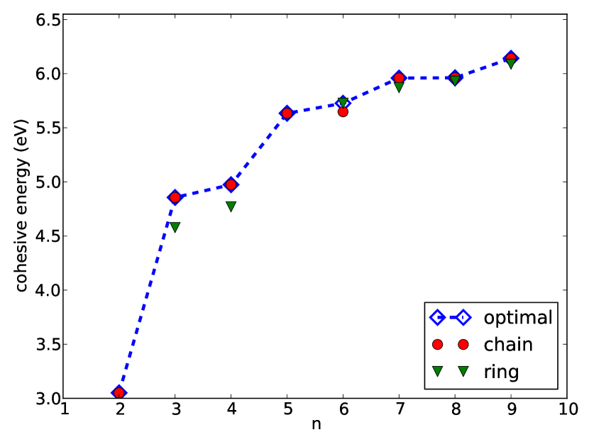
Figure 1: Cohesive energies of carbon clusters C₂ to C₉

Although $n=8$, $n=9$ chain geometries are optimal, they are nearly degenerate with the ring geometries. In the range of temperatures considered for nucleation (section 4), they are both within one $kT$. It is reasonable to conclude that the transition from chains to rings can occur at $n=8$.

Table 2: Optimal cohesive energies for C₂ to C₉

$n$	Geometry	$E_{c}$ (eV)
2	chain	3.051
3	chain	4.856
4	chain	4.974
5	chain	5.634
6	ring	5.727
7	chain	5.960
8	chain	5.962
9	chain	6.142

3.3 C₁₀ to C₂₀

The strain due to the curvature of carbon rings for $n\geq 10$ is sufficiently small that the extra C-C bond of the chain terminals becomes energetically preferable. The transition between aromatic states dominates in this regime, with the $4n+2$ cyclic rings showing pronounced peaks in stability (Fig.2). The $D_{nh}$ symmetry of the classical calculation is broken into a lower $D_{n/2h}$ due to Jahn-Teller distortion (Saito & Okamato 1999). The chain clusters show a repeating stair-step pattern, where stability is unchanged between an even and the preceding odd-numbered chain. The first fullerene-like states starting at C₁₈ are not as energetically stable as the rings. Optimal geometries and cohesive energies are given in Table 3.

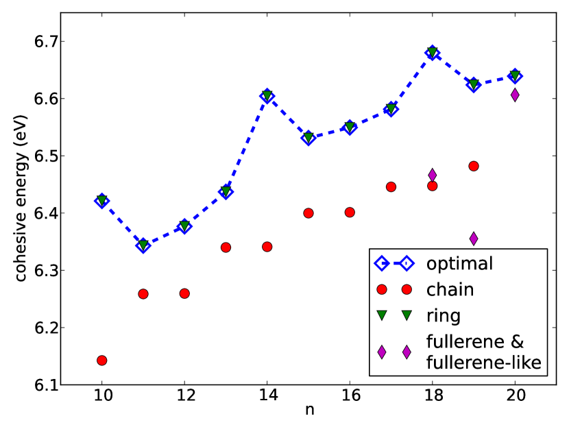
Figure 2: Cohesive energies of carbon clusters C₁₀ to C₂₀

Table 3: Optimal cohesive energies for C₁₀ to C₂₀

$n$	Geometry	$E_{c}$ (eV)
10	ring	6.421
11	ring	6.343
12	ring	6.377
13	ring	6.437
14	ring	6.604
15	ring	6.531
16	ring	6.549
17	ring	6.581
18	ring	6.680
19	ring	6.624
20	ring	6.639

3.4 C₂₁ to C₃₀

The exact transition from cyclic carbon to fullerenes or fullerene-like cages (hereafter fullerene-like) is an open question. No experimental evidence is available that conclusively shows where in this critical region the transition takes place, and different levels of theory are in disagreement (Handschuh et al. 1995; Helden et al. 1993).

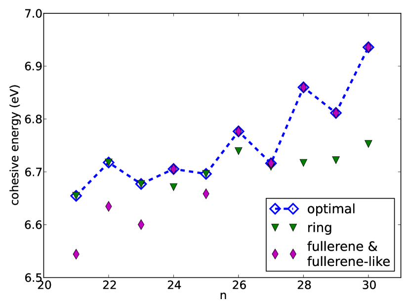
Figure 3: Cohesive energies of carbon clusters C₂₁ to C₃₀

Fig. 3 shows an initial continuation of the cyclic rings through the final aromatic structure C₂₂. The fullerene C₂₄ becomes the most stable configuration, although the odd-numbered C₂₅ fullerene-like suffers in stability from a dangling bond that returns the cyclic C₂₅ as the most stable configuration. C₂₇ is nearly degenerate in ring and fullerene-like geometries. The calculations performed here are in good agreement on the transition point with other studies using similar techniques (Kent 1999; Jones 1999). Compared to our second-order approximation of exchange-correlation energy functional (PBE), first-order approaches like local-density approximation (LDA) of the exchange-correlation energy functional prefer an earlier transition to fullerenes, whereas hybrid methods (B3LYP) prefer a later transition.

Continuing through particle number, the fullerenes and fullerene-like quickly outpace the cyclic structures, a trend that continues for the remainder of the clusters considered here. Optimal geometries and cohesive energies are given in Table 4.

Table 4: Optimal cohesive energies for C₂₁ to C₃₀

$n$	Geometry	$E_{c}$ (eV)
21	ring	6.655
22	ring	6.718
23	ring	6.677
24	fullerene	6.705
25	ring	6.696
26	fullerene	6.777
27	fullerene-like/ring	6.716
28	fullerene	6.860
29	fullerene-like	6.812
30	fullerene	6.936

3.5 C₃₁ to C₉₉

Fullerene and fullerene-like structures occupy the remainder of the optimally stable carbon clusters (Fig.4, Table 5). The binding energy is monotonically increasing, although there is a clear zig-zag pattern evident between the even- and odd-numbered fullerene clusters.

Odd numbered fullerene-like clusters, shown in Fig.5, are 2-coordinated at the appended atom, accounting for the clear instability in relation to the even numbered clusters. This extra atom prevents a fully closed cage structure associated with fullerenes. These clusters have been observed in the experiments with the fragmentation of C₆₀ (Deng et al. 1993; Kong et al. 2001), although they are generally regarded as intermediate states.

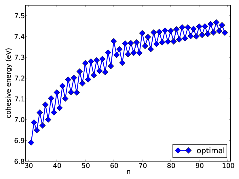
Figure 4: Cohesive energies of carbon clusters C₃₁ to C₉₉

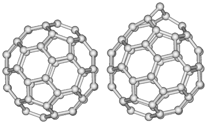
Figure 5: left: C₆₀ fullerene. right: C₆₁ fullerene-like cage with appended atom on top.

Strong peaks in stability are present at both C₆₀ and C₇₀, where the Isolated Pentagon Rule (IPR) is manifest (Kroto 1987). The most significant strain in fullerenes is due to the sub-optimal stability of the pentagon faces, which however are required to complete the geometry of the fullerene. IPR fullerenes keep pentagon faces maximally separated, minimizing the effect of pentagon strain and yielding a larger stability relative to the surrounding clusters.

A comparison of our results with other theoretical investigations as well as with experimental results is given in Table 6. The biggest differences are encountered when comparing our results to theoretical DFT calculations adopting less sophisticated pseudopotential (e.g., about 15% difference for C₄). Our results are comparable to within 1% to other DFT results adopting GGA pseudopotentials. Finally, comparison with experimental results show that our results (and in general DFT results) overestimate the cohesive energy by approximately 5%. Overall the agreement is quite good, even though the source of the systematic difference with experimental results deserves further investigation.

Table 5: Optimal cohesive energies for C₃₁ to C₉₉

$n$	Geometry	$E_{c}$ (eV)	$n$	Geometry	$E_{c}$ (eV)	$n$	Geometry	$E_{c}$ (eV)
31	fullerene-like	6.890	51	fullerene-like	7.194	71	fullerene-like	7.354
32	fullerene	6.987	52	fullerene	7.280	72	fullerene	7.398
33	fullerene-like	6.950	53	fullerene-like	7.214	73	fullerene-like	7.339
34	fullerene	7.034	54	fullerene	7.286	74	fullerene	7.420
35	fullerene-like	6.972	55	fullerene-like	7.235	75	fullerene-like	7.364
36	fullerene	7.072	56	fullerene	7.292	76	fullerene	7.423
37	fullerene-like	7.000	57	fullerene-like	7.229	77	fullerene-like	7.372
38	fullerene	7.103	58	fullerene	7.323	78	fullerene	7.429
39	fullerene-like	7.035	59	fullerene-like	7.258	79	fullerene-like	7.375
40	fullerene	7.131	60	fullerene	7.378	80	fullerene	7.427
41	fullerene-like	7.057	61	fullerene-like	7.312	81	fullerene-like	7.376
42	fullerene	7.163	62	fullerene	7.339	82	fullerene	7.434
43	fullerene-like	7.102	63	fullerene-like	7.274	83	fullerene-like	7.386
44	fullerene	7.193	64	fullerene	7.367	84	fullerene	7.444
45	fullerene-like	7.132	65	fullerene-like	7.315	85	fullerene-like	7.391
46	fullerene	7.201	66	fullerene	7.369	86	fullerene	7.444
47	fullerene-like	7.131	67	fullerene-like	7.322	87	fullerene-like	7.402
48	fullerene	7.232	68	fullerene	7.372	88	fullerene	7.437
49	fullerene-like	7.175	69	fullerene-like	7.322	89	fullerene-like	7.401
50	fullerene	7.272	70	fullerene	7.416	90	fullerene	7.448
51	fullerene-like	7.194	71	fullerene-like	7.354	91	fullerene-like	7.407
52	fullerene	7.280	72	fullerene	7.398	92	fullerene	7.449
53	fullerene-like	7.214	73	fullerene-like	7.339	93	fullerene-like	7.412
54	fullerene	7.286	74	fullerene	7.420	94	fullerene	7.459
55	fullerene-like	7.235	75	fullerene-like	7.364	95	fullerene-like	7.419
56	fullerene	7.292	76	fullerene	7.423	96	fullerene	7.468
57	fullerene-like	7.229	77	fullerene-like	7.372	97	fullerene-like	7.427
58	fullerene	7.323	78	fullerene	7.429	98	fullerene	7.455
59	fullerene-like	7.258	79	fullerene-like	7.375	99	fullerene-like	7.418

Table 6: Comparison of Cohesive energies $E_{c}$ for selected clusters

$n$	$E_{c}$ (this work)	$E_{c}$ (reference)	Method
3	4.86	4.60	Exp
3	4.86	4.85	DFTB
4	4.97	4.75	Exp
4	4.97	5.75	DFT(LDA)
5	5.63	5.25	Exp
6	5.72	5.76	DFT(GGA)
24	6.71	6.46	DQMC
24	6.71	6.75	DFT(GGA)
28	6.86	6.63	DQMC
32	6.99	6.88	DFT(GGA)
60	7.38	7.40	DFT(LDA)
60	7.38	7.38	DFT(GGA)
60	7.38	7.07	Exp
70	7.42	7.42	DFT(LDA)
70	7.42	7.10	Exp

4 Carbon dust nucleation

The principal application of the cohesive energies and structures computed in this work is for the calculation of the nucleation rate of carbonaceous dust in hydrogen-poor environments. The main example is formation of graphitic or amorphous-carbon grains in the inner layers of core-collapse supernovae, where the carbon to hydrogen number ratio is typically in the range $10^{6}:1$ to $10^{3}:1$ (Kozasa et al. 1989, 1991; Todini & Ferrara 2001; Fallest et al. 2011).

The deposition of carbon from the gas to the solid phase is a first order phase transition. The gas does not spontaneously go over from the old to the new phase in bulk. Between the metastable and stable phases there exists an energy barrier that makes a uniform and global phase change (associated to a density change) highly improbable. A far more energetically favorable pathway is the random formation of mirco-to-nanoscale density transition nuclei, a process known as nucleation.

The theory that follows utilizes the cluster model of nucleation. A bulk of $M$ particles exists in the gas phase, where a cluster of $n\ll M$ particles at higher density forms within a small region inside the bulk. In the following we consider both the classical thermodynamic theory of nucleation and the kinetic theory of nucleation. For the classical theory we will use both the standard capillary approximation (CNT-CAP) and our DFT-derived cohesive energies in the atomistic formulation (ANT-DFT) for evaluating the work energy of cluster formation. For the kinetic theory, we will use our DFT results for deriving the cluster concentrations and the monomer detachment rates (KNT-DFT).

4.1 Classical nucleation theory

In the classic nucleation theory, the rate at which new stable clusters are nucleated in the supersaturated gas per unit volume and time is given by:

$$J=z\gamma S^{*}C_{1}^{2}\sqrt{\frac{kT}{2\pi m_{0}}}e^{-W^{*}/kT}$$ (18)

where $z$ is the Zeldovich factor (see below), $\gamma$ is the sticking coefficient , $C_{1}$ is the equilibrium gas density of carbon at the given temperature, $m_{0}$ is the atomic mass of carbon, and $S^{*}$, $W^{*}$ are respectively the surface area and work of cluster formation, the star denoting that these quantities are associated with the cluster at the critical size (see below).

The work of cluster formation (WCF) is the energy necessary to form a cluster in the new phase from the constituents of the old one. The WCF of a cluster of size $n$ is given by

$$\begin{split}W_{n}&=G_{new,n}-G_{old,n}\\ &=-n\Delta\mu+G_{ex,n}\end{split}$$ (19)

where $G$ is the Gibbs free energy and $\Delta\mu=kT\ln S$ is the supersaturation Zettlemoyer (1969). T is the system temperature and S denotes the supersaturation ratio of vapor-to-equilibrium pressure $S=p/p_{e}$ (hereafter saturation).

Classical nucleation utilizes the capillary approximation to determine the excess Gibbs free energy $G_{ex,n}$

$$G_{ex,n}=\sigma_{n}S_{n}=\sigma_{n}c(nv_{0})^{\frac{2}{3}}$$ (20)

where $\sigma_{n}$ is the surface tension of the cluster, $c=S_{n}/V_{n}^{2/3}$ is a shape factor and $v_{0}$ is the volume of occupied by a single particle in the new phase. Clearly the capillary approximation is inadequate in the regime where $n$ is small, and where a spherical approximation for the molecular geometry is poor. Unfortunately, it is at this scale that nucleation is most significant for astrophysical refractory grains.

The capillary approximation offers a reasonably good description of nucleation when $n>>1$. In the case where $n\rightarrow 1$, the more exact atomistic model is required

$$G_{ex,n}=\lambda n-E_{n}$$ (21)

where $n\lambda$ is the work necessary to transfer $n$ particles from the old phase to the bulk of new one, and $E_{n}$ is the binding energy of the particle within the cluster. This form of $G_{ex,n}$ is valid for all $n$. However the difficulty of the theory is the determination of $E_{n}$, which is the result of complex chemical and quantum mechanical interactions within molecule. The focus of this work in section 3 was the evaluation of this term. The capillary approximation discards these difficulties in favor of a simple droplet model.

Eq.(21) allows the WCF to be expressed more precisely in the atomistic form

$$W_{n}=-n(\Delta\mu-\lambda)-E_{n}$$ (22)

To good approximation, $\lambda$ can be treated as an intensive property of the material. As $\Delta\mu$ is given in terms of the thermodynamic variables ($T$, $S$) of the system, this leaves the binding energy $E_{n}$ as the only unknown quantity in determining the WCF. Our DFT calculations allow us to compute $E_{n}$ directly for small clusters, without the need to recourse to the capillary approximation.

The classical nucleation rate (Eq. 18) is given in terms of the surface area and WCF of the cluster at the critical size $n^{*}$. The value of $n^{*}$ is the size at which the $W_{n}$ is maximum. Clearly, determination of the critical size $n^{*}$ is essential. In the capillary approximation $W_{n}$ is a smooth, continuous function of $n$, and determination of $n^{*}$ is accomplished with elementary analysis. However, in the case of Eq.(22) the $W_{n}$ have no known analytic form, and determination of $n^{*}$ must be done by direct inspection of available values.

A more concise form of Eq.(18) can be given using the monomer attachment rate for a cluster of size $n$ as

$$f_{n}=\gamma S_{n}C_{1}\sqrt{\frac{kT}{2\pi m_{0}}}$$ (23)

and the $n$-cluster concentration as

$$C_{n}=C_{1}e^{-W_{n}/kT}$$ (24)

The steady-state nucleation rate is then

$$J_{s}=zf^{*}C^{*}$$ (25)

The Zeldovich factor $z$ is is present to account for back-decay of the supercritical clusters. In the classical theory, it takes the approximate form

$$z=\left[\left(\frac{-1}{2\pi kT}\right)\left(\frac{d^{2}W}{dn^{2}}\bigg{|}_{n=n^{*}}\right)\right]^{1/2}$$ (26)

Evaluation using the capillary approximation from Eq.(20) gives

$$z=\sqrt{\frac{W^{*}}{3\pi kTn^{*}}}$$ (27)

In the atomistic case, the derivatives in Eq.(26) are ill-defined. Recourse to the kinetic formulation (see Lewis & Anderson 1978) shows that $z$ can be given in terms of $C_{n}$

$$z=\left(\sum_{n=1}^{h}\frac{C^{*}}{C_{n}}\right)^{-1}$$ (28)

where $h>n^{*}$ is a reasonable cut-off of the summation (see below).

4.2 Kinetic nucleation theory

A more precise treatment of nucleation is given by the kinetic theory, first formulated by Becker (Becker & Döring 1935). Clusters are assumed to form in a bath of abundant monomers, their size changing by no more than one atom at a time. The steady state nucleation rate is given in terms of attachment and detachment rates ($f_{n}$ and $g_{n}$, respectively):

$$J=f_{1}C_{1}\left[1+\sum_{n=2}^{h}\frac{g_{2}g_{3}...g_{n}}{f_{2}f_{3}...f_{n}}\right]^{-1}$$ (29)

In this formulation no recourse to thermodynamics is required, and the simplifying assumptions of CNT can be discarded provided $f_{n}$ and $g_{n}$ are known. In principle, the attachment and detachment rates must be known at any size $n$ ($h=\infty$). However, if a critical cluster $n^{*}$ is defined for the size at which $f_{n}=g_{n}$, the summation in Eq.(29) can be truncated at $h=2n^{*}$ (e.g. Kashchiev 2000).

The kinetic nucleation theory is readily amenable to adoption of our DFT-derived cohesive energies since

$$g_{n}\propto e^{(W_{n}-W_{n-1})/kT}\propto e^{[\lambda-(E_{n}-E_{n-1})]/kT}$$ (30)

A close look to our results, however, reveals that the ratio $f_{n}/g_{n}$ keeps oscillating around unity, preventing us to identify the critical cluster size in the kinetic sense. However, it is possible to avoid this difficulty by reintroducing the cluster concentrations $C_{n}$ defined in Eq.(24), since

$$C_{n}=C_{1}e^{W_{n}/kT}=C_{1}\frac{f_{1}f_{2}f_{3}\dotso f_{n-1}}{g_{2}g_{3}g_{4}\dotso g_{n}}$$ (31)

Eq.(29) takes on the simple form

$$J_{s}=\left(\sum_{n=1}^{h}\frac{1}{f_{n}C_{n}}\right)^{-1}$$ (32)

Inspection of the above reveals a clear dominance of the term at $n=n^{*}$, where $n^{\star}$ is here defined as the value of $n$ that maximized $W_{n}$, as in CNT. Truncating the summation at $h=2n^{*}$ has negligible effect on the result.

Values for bulk sublimation energy $\lambda$, surface tention $\sigma$, and carbon molecule mass $m_{0}$ are those used in Fallest (2012).

4.3 Results

4.3.1 Work of cluster formation

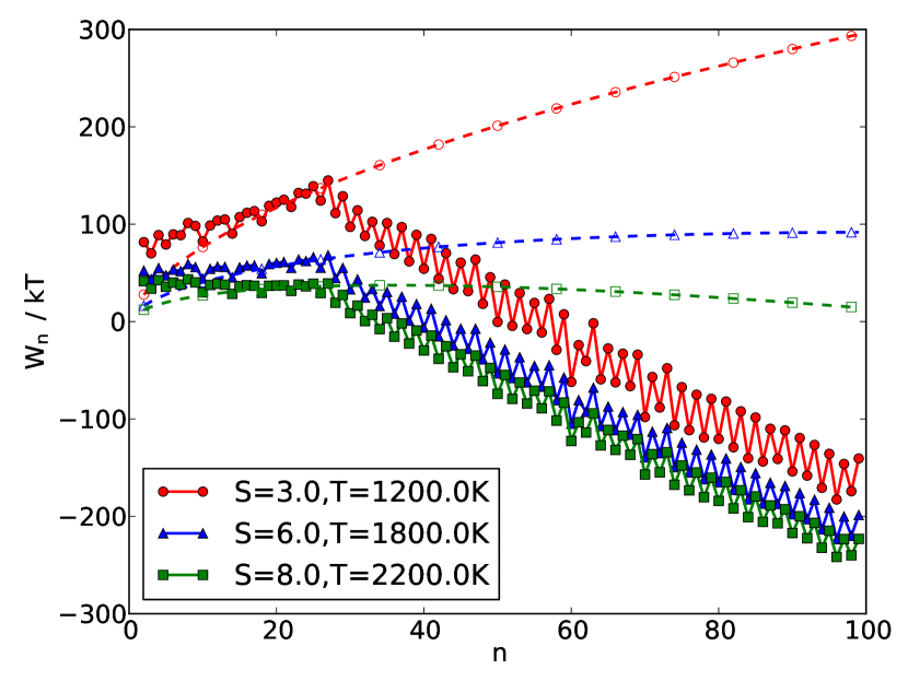
Figure 6: Work of Cluster Formation for three values for temperature, saturation. Solid curves are from this work, dashed curves are $W_{n}$ in CNT. $W_{n}$ given per $kT$

Fig.(6) shows the WCF for different values of temperature and saturation in both the CNT and the accurate atomistic cluster formation energy using the results of DFT calculations. The overall trend of the atomistic evaluation changes nearly linearly on both sides of the fullerene transition. Higher temperatures and saturations give a much slower growth before the fullerenes. It is in this regime where CNT is most near the atomistic case. The classical WCF coincides most closely at the high-$n$ ring structures. CNT estimates lower WCFs at the low chains.

The most striking divergence between CNT and the atomistic case is at the fullerene transition. Here the is a distinct change in the trend of the cluster energies. At low temperatures and saturations this is clearly the critical size. At higher temperatures and saturations, the critical size is located at a lower cluster size, although a distinct transition into the fullerenes is still apparent. This change arises from the properties of the fullerene in relation to the previous geometries. In particular, the fullerene is 3-coordinated (compared to the 2-coordinated rings) and addition carbon atoms releases more energy than in the 2-coordinated case. As seen below in the results for the critical cluster size, the fullerene transition (and, to a lesser extent, the ring transition) provide a natural critical size past which growth in the new phase is spontaneous.

4.3.2 Critical cluster size

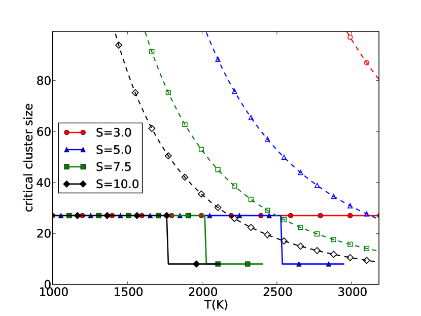
Figure 7: Critical cluster size $n^{*}$ as a function of temperature at different values of saturation. Solid curves are results of this work, while dashed curves and symbols are derived from CNT.

Critical cluster sizes in the classical and precise atomistic case are given in Fig.(7). Critical sizes in both cases are determined by selecting the value of $n$ for the maximum value of the WCF, if such a maximum exists for $2<n<99$. CNT gives every-increasing values for the critical size as the temperature falls. In the atomistic case the maximum critical size at $n^{*}$ is consistent at $n^{*}=27$ for a wide range of temperature and saturation. The critical size falls in both models with increasing temperature, however the atomistic case gives a minimum critical size of $n^{*}=8$.

At higher temperatures and saturations, the WCF is maximum at $n=2$, implying that a catastrophic seeding of the new phase should take place. In practice, since at high temperatures nucleation is fast, the gas phase is depleted at very small saturation when $n^{*}>2$, and saturation never reaches values for which catastrophic nucleation occurs.

4.3.3 Nucleation rates

As discussed above, we will adopt three methodologies to compute the nucleation rate. In the first method, named CNT-CAP we adopt the capillary approximation within the classical nucleation theory. Nucleation is computed from Eq.(18) with the Zeldovich factor from Eq.(27), surfaces calculated for spherical uniformly filled grains, and WCF from the capillary approximation Eq.(20). The second methodology, named ANT-DFT still adopts the classical nucleation theory, but the capillary approximation is replaced by our DFT results on the clusters’ cohesive energies. The WCF is computed from Eq.(22), and the cluster surfaces derived from the most stable configurations in DFT. In practice, we compute the surfaces with the formula

$$S_{n} =2\pi r_{C}nl+2\pi r_{C}^{2}$$ (33)

$$S_{n} =2\pi r_{C}(n-1)l$$ (34)

$$S_{n} =12A_{p}+(n/2-10)A_{h}$$ (35)

for the chain, ring, and fullerene (Adams et al. 1994) areas respectively. $l$ is an assumed bond length, and $r_{C}$ is the carbon atom radius. We take as $l=1.4\text{\AA}$ and $r_{C}=1\text{\AA}$. The Zeldovich factor is computed atomistically using Eq.(28).

Finally, we compute the nucleation rate with the full kinetic theory, and we label these results as KNT-DFT. The nucleation rate in this case is computed with Eq.(32), where the cluster concentrations are derived according to Eq.(24) and making use of our DFT-derived cohesive energies.

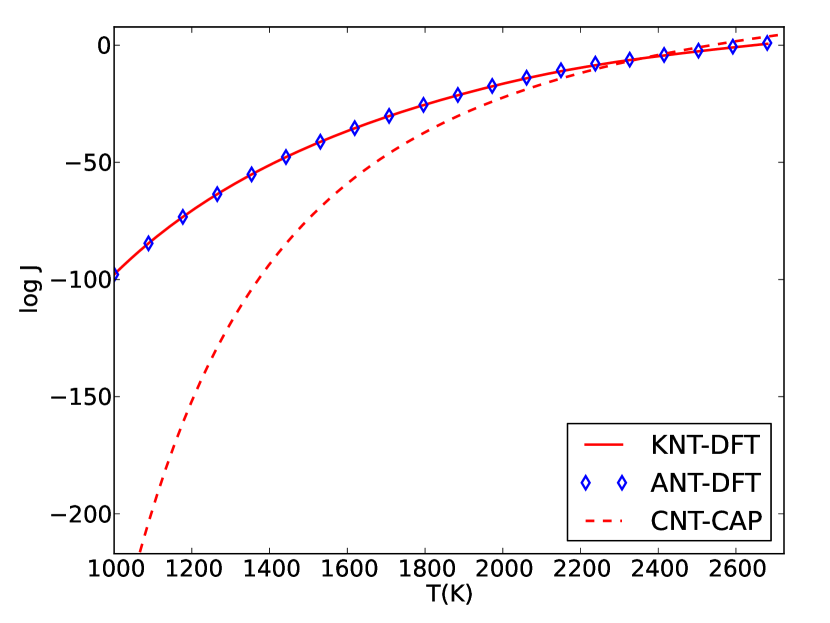
Figure 8: Nucleation rates for a single saturation using CNT-CAP (dashed), ANT-DFT (diamond), & KNT-DFT (solid).

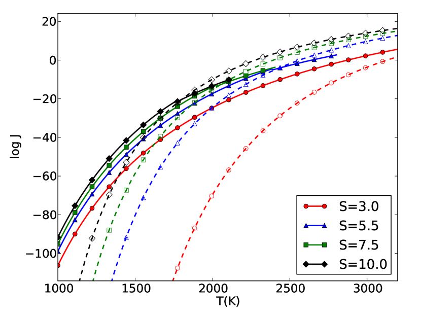
Figure 9: Nucleation rates at different saturations using ANT-DFT(solid, filled) and CNT-CAP (dashed, open).

A comparison of CNT-CAP, ANT-DFT, and KNT-DFT nucleation rates is plotted in Fig.  8. ANT-DFT and KNT-DFT rates agree to very high order. Expanding Eq.(25) with Eq.(28)

$$J_{cl}=zf^{*}C^{*} =\left[\sum_{n=1}^{h}\left(\frac{C^{*}}{C_{n}}\right)\right]^{-1}f^{*}C^{*}$$

$$=\left[\sum_{n=1}^{h}\left(\frac{1}{C_{n}}\right)\right]^{-1}f^{*}$$

$$=\left[\sum_{n=1}^{h}\left(\frac{1}{f^{*}C_{n}}\right)\right]^{-1}$$

Cleary this only differs from Eq.(32) by the the constant $f^{*}$ in the summation. The $f_{n}$’s vary much more slowly than the $C_{n}$’s, and the difference between the two sums is negligible.

Since the ANT-DFT and KNT-DFT results are in good agreement with each other, we only show in the following the results of ANT-DFT. This is not a trivial result and it is particularly useful for numerical implementations of nucleation, since the prescription of ANT-DFT is much faster than KNT-DFT, especially at large critical sizes.

ANT-DFT rates and CNT-CAP rates are compared for a set of saturations in Fig.(9). Nucleation at lower temperatures is faster than in the capillary model, due to the much smaller critical size given by DFT. As the critical size predicted by the two calculations converge the rates of the methods track better. At large temperatures and saturations nucleation is suppressed. In this regime DFT predicts no critical size beyond the dimer. Transition between the two phases is spontaneous. Lower saturations allow higher nucleation temperatures.

5 Conclusions and Discussion

We performed empirical global geometry optimization on carbon clusters $n=2$ to $n=99$ using a combination of search algorithms to find lowest-energy candidate clusters. We then applied local geometry optimization and binding energy calculation using the DFT code Quantum Espresso to determine the precise ground state. These results are applied to accurate atomistic nucleation theory and compared with the results of classical nucleation theory.

Where there is overlap, our results for the geometries and energies conform well to previous studies. We find good agreement with calculations performed using similar DFT methods (see Table 6). Higher energies than quantum Monte Carlo techniques are found, although we find a similar ring-to-fullerene transition pattern (Kent 1999). As expected, our results for small clusters are consistently lower than corresponding LDA methods, which are known to overestimate energies and bond strengths. All DFT methods overestimate the energies compared to experimental values for small clusters.

Low-$n$ clusters are mostly chains, with C₆ the only ring structure due to the strong stability of Huckle aromaticity. Carbon rings begin to form at C₁₀ and continue up to C₂₇. These rings are initially distorted and show lower symmetry than their counterparts in classical evaluations, but this distortion declines with larger $n$. Fullerene and fullerene-like structures start at C₂₄, and form all ground state configurations from C₂₈ to C₉₉.

Even though the calculations were performed at zero pressure, they are expected to provide an excellent approximation for the typical pressures at which astrophysical nucleation takes place (less than one barye). As an example, consider the $n=92$ fullerene. It can be re-casted in an onion structure with an $n=32$ fullerene inside a $n=60$ buckminsterfullerene. This nested structure has a lower total binding energy by approximately $10$ eV or $1.9\times 10^{-}{11}$ erg. Since the volume of the C₉₂ fullerene is of order $10^{-22}$ cm², a very large pressure of approximately $10^{11}$ barye is required so that the more compact onion structure has a lower enthalpy then the bigger C₉₂ fullerene.

Critical cluster sizes and nucleation rates were calculated with these results and compared to the rates obtained with the classical capillary approximation. We find that the critical cluster size consistently falls near the two geometry transitions (chain-to-ring, ring-to-fullerene), while it varies continually as a function of temperature and saturation adopting the capillary approximation. As a consequence, our ANT-DFT results yield larger nucleation rates at low temperature and saturations, the regimes in which CNT-CAP predicts very large critical clusters. In support of our conclusion, previous work has shown that ANT offers a richer and more natural nucleation description than CNT by accounting for irregular cluster geometries (Kashchiev 2012).

Nucleation rates at higher temperatures and saturations tend to be similar, as the difference in critical cluster size between the exact case and the capillary approximation becomes smaller. An important result particularly relevant for numerical implementations is that the nucleation rates do not depend on the use of the classical or kinetics frameworks. The more computational intensive kinetic theory yields rates only marginally different from the classical thermodynamic framework, as long as the work for cluster formation, the cluster surfaces, and the Zeldovich factor are computed with DFT cohesive energies instead of with the capillary approximation.

References

- Adams et al. (1994) Adams G. B. et al. 1994, Journal of Chemical Physics, 98, 9465
- Bauschlicher et al. (2010) Bauschlicher, C. W., Jr., Boersma, C., Ricca, A., et al. 2010, ApJS, 189, 341
- Becker & Döring (1935) Becker R. & Döring 1935, Annalen der Physik, 416, 719
- Blum & Wurm (2008) Blum J. & Wurm G. 2008, Annual Review of Astronomy and Astrophysics, 46, 21
- Brenner (1990) Brenner, D W. 1990, Physical Review B, 42, 9458
- Brinkmann & Dress (1997) Brinkmann G. & Dress A. W. M. 1997, Journal of Algorithms, 23, 345
- Cherchneff & Dwek (2009) Cherchneff I. & Dwek E. 2009, Astrophysical Journal, 703, 642
- Cherchneff & Dwek (2010) Cherchneff I. & Dwek E. 2010, Astrophysical Journal, 713, 1
- Deng et al. (1993) Deng J.P. et al. 1993, Journal of Chemical Physics, 92, 11575
- Donn & Nuth (1985) Donn B. & Nuth J. A. 1985, Astrophysical Journal, 288, 187
- Draine (2003) Draine B. T. 2003, Astrophysical Journal, 598, 1017
- Drowart et al. (1959) Drowart J. et al. 1959, Journal of Chemical Physics, 31, 1131
- Fallest et al. (2011) Fallest D. W. et. al. 2011, Monthly Notices of the Royal Astronomical Society, 418, 571
- Fallest (2012) Fallest D. W. 2012 Kinetic Nucleation Theory and Thermal Fluctuations in the Formation of Cosmic Dust, North Carolina State University
- Gall et al. (2014) Gall, C. et al. 2014, Nature, 511, 326
- Giannozzi et al. (2009) Giannozzi P., et al. 2009, Journal of Physics: Condensed Matter, 39, 21. http://www.quantum-espresso.org
- Goedecker (2004) Goedecker S. 2004, Journal of Chemical Physics, 120, 21
- Goumans & Bromley (2012) Goumans, T. P. M., & Bromley, S. T. 2012, MNRAS, 420, 3344
- Grimme (1997) Grimme S. 1997, Journal of Molecular Structure, 398, 301
- Handschuh et al. (1995) Handschuh H. et.al. 1995, Physical Review Letters, 74, 7
- Helden et al. (1993) Helden G. et al. 1993, Chemical Physics Letters, 204, 1
- Hohenberg & Kohn (1964) Hohenberg P. & Kohn W. 1964, Physical Review, 136, 3B
- Johnston (2002) Johnston, R. L. 2002, Atomic and Molecular Clusters, Taylor and Francis, London, UK, 2002
- Jones (2001) Jones A.P. 2001, Philosophical Transactions of the Royal Society London A, 369, 1787
- Jones (1999) Jones R.O. 1998, Journal of Chemical Physics, 110, 11
- Kashchiev (2000) Kashchiev D. 2000, Nucleation, Butterworth-Heinemann
- Kashchiev (2008) Kashchiev D. 2008, Journal of Chemical Physics, 129, 164701
- Kashchiev (2012) Kashchiev D. 2012, Crystal Growth & Design, 12, 3257
- Kent (1999) Kent P.R.C. 1999, Techniques and Applications of Quantum Monte Carlo, University of Cambridge
- Kobayashi et al. (1992) Kobayashi K. et al. 1992, Physical Review B., 45, 13690
- Kohn & Sham (1965) Kohn W. & Sham L. J. 1965, Physical Review, 140, 1133
- Kong et al. (2001) Kong Q. et al. 2001, International Journal of Mass Spectrometry, 209, 1
- Kozasa et al. (1989) Kozasa, T., Hasegawa, H., & Nomoto, K. 1989, ApJ, 344, 325
- Kozasa et al. (1991) Kozasa, T., Hasegawa, H., & Nomoto, K. 1991, A&A, 249, 474
- Kroto (1987) Kroto H. W. 1987, Nature, 329, 8
- Lazzati (2008) Lazzati, D. 2008, Monthly Notices of the Royal Astronomical Society, 384, 165
- Lewis & Anderson (1978) Lewis B. & Anderson J. C. 1978 Nucleation and Growth of Thin Films, Academic Press
- Martin (2004) Martin R. M. 2004, Electronic Structure, Cambridge University Press
- McEwen & Schleyer (1986) McEwen A. B. & Schleyer P. R. 1986, Journal of Organic Chemistry, 51, 4357
- Menon et.al. (1993) Menon G. & Subbaswamy K. R. & Sawraire M., 1993, Physical Review B, 48, 8398
- Perdew et al. (1992) Perdew J. P. et al. 1992, Physical Review B, 46, 6671
- Perdew et al. (1996) Perdew J. P., Burke K., & Ernzerhof M. 1996, Physical Review Letters, 77, 3865
- Ravagnan et al. (2002) Ravagnan L. et al. 2002, Physical Review Letters, 89, 28
- Saito & Okamato (1999) Saito M. & Okamoto Y. 1999, Physical Review B, 60, 12
- Saito & Oshiyama (1991) Saito S. & Oshiyama A. 1991, Physical Review B, 44, 11532
- Speck et al. (2008) Speck, A. K., Whittington, A. G., & Tartar J. B. 2008, Astrophysical Journal Letters, 687, L91
- Spoon et al. (2006) Spoon H. W. W. et al. 2006, Astrophysical Journal, 638, 759
- Todini & Ferrara (2001) Todini, P. & Ferrara, A. 2001, Monthly Notices of the Royal Astronomical Society, 325, 726
- Wales & Doye (1997) Wales D. J. & Doye P. K. J. 1997, Journal of Physical Chemistry A, 101, 28
- Weingartner & Draine (2001) Weingartner J. C & Draine B. T., Astrophysical Journal, 528, 296
- Whittet (2003) Whittet D. C. B. 2003, Dust in the Galactic Environment, Institute of Physics Publishing
- Williams et al. (1990) Williams, P. M., van der Hucht, K. A., The, P. S., & Bouchet, P. 1990, Monthly Notices of the Royal Astronomical Society, 247, 18
- Varricatt et al. (2004) Varricatt W. P., Williams P. M., & Ashok N. M. 2004, Monthly Notices of the Royal Astronomical Society, 351, 1307
- Zettlemoyer (1969) Zettlemoyer, A. C. 1969, Nucleation, Dekker