Analytic solutions of topologically disjoint systems

Abstract

We describe a procedure to solve an up to $2N$ problem where the particles are separated topologically in $N$ groups with at most two particles in each. Arbitrary interactions are allowed between the (two) particles within one group. All other interactions are approximated by harmonic oscillator potentials. The problem is first reduced to an analytically solvable $N$-body problem and $N$ independent two-body problems. We calculate analytically spectra, wave functions, and normal modes for both the inverse square and delta-function two-body interactions. In particular, we calculate separation energies between two strings of particles. We find that the string separation energy increases with $N$ and interaction strength.

I Introduction

Analytic models were unavoidable in physics before the advent of computers. This forced researchers to extract the essence of the problems and design the models to catch the crucial properties. Appropriately done these simplifications delivered deep insight and the necessary realistic results. Computers are extremely useful to provide solutions of more and more complicated problems. Advanced research is then almost by definition forced to push implementations to the limit of the available computer capacity.

The increased complexity of problems combined with large numerical calculations require larger efforts to understand and develope an intuition for the underlying physics. Getting the deeper insight is more difficult for complicated problems, but nevertheless very desirable for several reasons. Beside the direct usefulness of basic understanding, it is also efficient in construction of improved algorithms, which in turn would allow investigation of even more complicated problems.

We recapitulate briefly a number of important reasons to employ suitable analytic methods. First, model construction must concentrate on the crucial features, and thus formulate and order the issues according to importance. Second, in many perturbative approaches in physics the potentials are expanded to second order in coordinates or momenta, and the emerging harmonic oscillator problems are analytic. Third, a problem can be beyond even present day computer capacity. Fourth, advanced numerics can be greatly improved by combination with analytic tools and insight. Fifth, analytic models can hardly be overestimated as a tool in teaching on all levels. Sixth, present experimental frontline research on cold atomic gases employ unprecedentedly simple (almost) analytically solvable potentials bloc08 .

The harmonic oscillator is the simplest and most useful analytic potential at our disposal and this has been exploited throughout the history of physics. A relevant example dating all the way back to 1926 is by Werner Heisenberg who used harmonic Hamiltonians to gain insight into the many-body problem heisenberg1926 (within a year of him inventing the new quantum theory). Later on the harmonic oscillator was instrumental in providing insights for models of the atomic nucleus goep55 . Harmonic interactions have also been used as a replacement for Coulomb potentials in atoms in order to gain analytical insights (the so-called Moshinsky atom or pseudoatom) moshinsky1968 ; moshinsky1985 . These models continue to produce new insights into aspects of atomic systems such as the density matrix amovilli2003 ; schilling2013a , correlations kestner1962 ; taut1993 ; lopez2006a ; lopez2006b ; laguna2011 and entropy amovilli2004 , density functionals riveros2012a , and entanglement properties pipek2009 ; yanez2010 ; bouvrie2012 ; riveros2012b ; koscik2013 ; riveros2014 ; bouvrie2014 . Harmonic models have been a subject of great interest in several other fields including quantum dots johnson1991 , quantum statistics liang2012 ; schilling2013b , black holes thermodynamics bombelli1986 ; srednicki1993 , and recently also area laws and entanglement in quantum many-body systems eisert2010 .

In the field of cold atomic gases the harmonic oscillator method has also served as an important model to gain insights. For instance, it has been used extensively as a starting point for path integral calculations of quantum gas properties bros97 ; zalu00 ; yan03 ; gajd06 ; tempere1997 . More recently, an $N$-body model for harmonically interacting particles in an external harmonic confining potential has been solved arms11 ; arms12 , and the spectra have been used to investigate thermodynamics and virial expansions arms12a ; arms12b . All these studies attest to the versatility of the harmonic approach as an analytical tool that can address even advanced frontline research questions.

A recent frontier in ultracold atomic gases is the creation of ultracold polar molecules lahaye2009 ; carr2009 with long-range interactions that hold great promise for greating some unique exotic quantum systems carr2009 ; baranov2008 . To avoid strong dipolar loss due to the attractive head-to-tail interactions, the dipoles should be confined to lower dimensional geometries such as tubes or layers, and a layered system of dipoles was recently experimentally realized mira11 . In such a system one expects the formation of chains of dipoles which are bound structures across several layers wang06 ; arms-dip12 ; barbara2011 ; arms-dip13 . Similarly, in one-dimensional tubes one also expects this bound state formation klawunn2010 ; barbara2011 ; artem-dip2013 . This chain formation takes place in a topologically disjoint system as the layers or tubes are physically disconnected when tunneling between them is negligible. However, they still provide a very interesting physical system as the dipolar interactions are long-range and act between physically disconnected parts of the system. Here we consider some general models that allow an analytical approach to such topologically disjoint geometries.

More generally, the purpose of the present paper is to discuss an analytic model which reduces a $2N$ problem in a non-trivial geometry with disjoint regions to an approximate but analytic $N$-body problem and $N$ individual two-body problems. The particles must pairwise have the same masses but the in-pair interaction can be arbitrary. The same four two-body oscillator interactions are preferred between two such pairs. Otherwise there are no constraints on masses and arbitrary oscillator intereractions are allowed. A seperable model like the one we discuss here has been studied recently within the context of exactly solvable models karwowski2004 ; karwowski2008 and applied as a model of two-electron atoms and molecules karwowski2010 . In the current work we will be applying this kind of Hamiltonian to other model systems that are of relevance for neutral atoms in cold atomic gases.

The paper is organized as follows. In Section II we derive the conditions for the huge simplification obtained by decoupling the different degrees of freedom. In section III we specialize to analytic two-body problems, and in Section IV we present a number of corresponding examples for illustrations. Finally in Section V , we briefly summarize, conclude and give perspectives.

II Method

We consider a system of particles which can be divided into $N$ groups where each consists of one or two particles. A priori, all particles may be identical or different, and any spatial dimension is allowed. The two-body interactions between all the topologically separated groups of particles are assumed to be harmonic oscillators. In addition, we allow completely arbitrary interactions between the pairs of particles within each of the $N$ groups. Identical particles must obey Fermi or Bose symmetry relations, but the group distinction must be maintained. The perhaps artificially appearing grouping and the related conditions arise from anticipating a strongly simplifying decoupling of the many degrees of freedom. The corresponding additional decoupling conditions are derived in the first subsection, and specific features of the solutions are discussed in the second subsection.

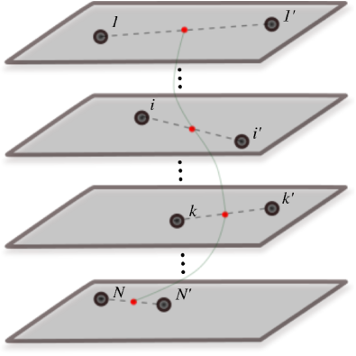
Figure 1: (Color online) Schematic picture of a possible $2D$ layer geometry with two particles in each layer (for instance $i$ and $i^{\prime}$). The pairwise intra-layer relative motion are independent of other pairs, and as well independent of the motion of their intra-layer center-of-masses. The particles could be constrained to stay on a one-dimensional curve within each layer reducing the problem to $1D$. The particles may also be allowed to move freely in all three dimensions, but for the decoupling to work we insist that only $i-i^{\prime}$ pairs can have arbitrary relative two-body interactions.

The required distinction between particles and interactions can be achieved by geometrically separated systems. The most obvious possibilities are series of separate two-dimensional layers or one-dimensional tubes where each layer or tube is occupied by one or two particles. We provide a visualization in fig. 1. The inter-layer and/or inter-tube two-body interactions then must be of harmonic oscillator form whereas arbitrary intra-layer and/or intra-tube two-body interactions are allowed. In addition one-body harmonic oscillator potentials acting on each of the particles are also allowed. The restrictive fundamental conditions may even be possible in some three-dimensional structures. Imagine a lattice with up to two particles per site with arbitrary on-site interactions, and harmonic potentials between particles on different sites.

II.1 Hamiltonian

The $N$ groups are labeled by $k=1,2,3,...,N$ and the two particles in each group are labeled by $k$ and $k^{\prime}$, where we first assume two particles in all $N$ groups. To simplify the discussion we shall refer to the system as a series of $N$ doubly occupied layers. Only $k$ and $k^{\prime}$ are allowed arbitrary interactions, while two-body individual harmonic oscillator potentials are assumed for any of the other interactions. The Hamiltonian, $H$, of this $N$-layer system is then

$$H=-\frac{\hbar^{2}}{2}\sum_{k=1}^{N}\left(\frac{1}{m_{k}}\nabla_{k}^{2}+\frac{1}{m_{k^{\prime}}}\nabla_{k^{\prime}}^{2}\right)+V^{(shift)}$$

$$+\sum_{k=1}^{N}V_{k}(\mathbf{r}_{k}-\mathbf{r}_{k^{\prime}})+\frac{1}{2}\sum_{k=1}^{N}\omega_{0k}^{2}\left(m_{k}r_{k}^{2}+m_{k^{\prime}}r_{k^{\prime}}^{2}\right)$$

$$+\frac{1}{2}\sum_{i=1}^{N-1}\sum_{k=i+1}^{N}\left[\mu_{ik}\omega_{ik}^{2}\left(\mathbf{r_{i}}-\mathbf{r_{k}}\right)^{2}+\mu_{ik^{\prime}}\omega_{ik^{\prime}}^{2}(\mathbf{r_{i}}-\mathbf{r_{k^{\prime}}})^{2}\right.$$

$$\left.+\mu_{i^{\prime}k}\omega_{i^{\prime}k}^{2}(\mathbf{r_{i^{\prime}}}-\mathbf{r_{k}})^{2}+\mu_{i^{\prime}k^{\prime}}\omega_{i^{\prime}k^{\prime}}^{2}(\mathbf{r_{i^{\prime}}}-\mathbf{r_{k^{\prime}}})^{2}\right]\;,$$ (1)

where $\mathbf{r}_{k}$ and $m_{k}$ are coordinate and mass of particle $k$, $\mu_{ik}=m_{i}m_{k}/(m_{i}+m_{k})$ is the reduced mass between particles $i$ and $k$, $V_{k}$ is the intra-layer interaction between particles $k$ and $k^{\prime}$ in the $k$th layer, $\omega_{0k}=\omega_{0k^{\prime}}$ is the one-body external field frequency, $\omega_{ik}$ is the harmonic frequency between the particles $i$ and $k$ in the layers $i$ and $k$, and $V^{(shift)}$ is a constant zero-point energy shift which is needed to compare with experimental results. Numerically, $V^{(shift)}$ is the sum of the individual interactions, $v^{(shift)}_{ik}$, between particles $i$ and $k$, that is

$$V^{(shift)}=$$

$$\sum_{i=1}^{N-1}\sum_{k=i+1}^{N}\left(v^{(shift)}_{ik}+v^{(shift)}_{i^{\prime}k}+v^{(shift)}_{ik^{\prime}}+v^{(shift)}_{i^{\prime}k^{\prime}}\right).$$ (2)

which are chosen to fit the energies of the individual two-body systems. All these definitions are completed by repeating with primes on each of the indices as applied in the equations. The different terms are divided and explicitely written according to layers and thereby reducing the summation index to run over layers.

We transform the coordinates in the different layers to relative, $\mathbf{\tilde{r}_{k}}$, and center-of-mass two-body coordinates, $\mathbf{R_{k}}$. Defining $M_{k}=m_{k}+m_{k^{\prime}}$, the transformations both ways become

$$\mathbf{\tilde{r}_{k}} = \mathbf{r_{k}}-\mathbf{r_{k^{\prime}}}\;;\;\;\;\mathbf{R_{k}}=\frac{m_{k}\mathbf{r_{k}}+m_{k^{\prime}}\mathbf{r_{k^{\prime}}}}{M_{k}}\;,$$ (3)

$$\mathbf{r_{k}} = \mathbf{R_{k}}+\frac{m_{k^{\prime}}}{M_{k}}\mathbf{\tilde{r}_{k}}\;;\;\;\;\mathbf{r_{k^{\prime}}}=\mathbf{R_{k}}-\frac{m_{k}}{M_{k}}\mathbf{\tilde{r}_{k}}\;.$$ (4)

Inserting these transformations into the Hamiltonian in eq. (1) leads to many terms. We consider first the one-body terms from the kinetic energy operators and external fields, that is

$$\frac{1}{2}\left(\omega_{0k}^{2}(m_{k}r_{k}^{2}+m_{k^{\prime}}r_{k^{\prime}}^{2})-\frac{\hbar^{2}}{m_{k}}\nabla_{k}^{2}-\frac{\hbar^{2}}{m_{k^{\prime}}}\nabla_{k^{\prime}}^{2}\right)=$$

$$\frac{1}{2}\left(\omega_{0k}^{2}(M_{k}R_{k}^{2}+\mu_{kk^{\prime}}\tilde{r}_{k}^{2})-\frac{\hbar^{2}}{M_{k}}\nabla_{R_{k}}^{2}-\frac{\hbar^{2}}{\mu_{kk}}\nabla_{\tilde{r}_{k}}^{2}\right)\;.$$ (5)

Then we transform the two-body oscillator terms in eq. (1) while assuming $\omega_{kk}=0$, $\omega_{ik}=\omega_{ki}$ and also for the primed indices. We find with the substitution in eq. (4) that

$$\frac{1}{4}\sum_{i=1}^{N}\sum_{k=1}^{N}[\mu_{ik}\omega_{ik}^{2}(\mathbf{r_{i}}-\mathbf{r_{k}})^{2}+\mu_{i^{\prime}k}\omega_{i^{\prime}k}^{2}(\mathbf{r_{i^{\prime}}}-\mathbf{r_{k}})^{2}$$

$$+\mu_{ik^{\prime}}\omega_{ik^{\prime}}^{2}(\mathbf{r_{i}}-\mathbf{r_{k^{\prime}}})^{2}+\mu_{i^{\prime}k^{\prime}}\omega_{i^{\prime}k^{\prime}}^{2}(\mathbf{r_{i^{\prime}}}-\mathbf{r_{k^{\prime}}})^{2}]$$

$$=\frac{1}{4}\sum_{i=1}^{N}\sum_{k=1}^{N}(\mathbf{R_{i}}-\mathbf{R_{k}})^{2}[\mu_{ik}\omega_{ik}^{2}$$

$$+\mu_{i^{\prime}k}\omega_{i^{\prime}k}^{2}+\mu_{ik^{\prime}}\omega_{ik^{\prime}}^{2}+\mu_{i^{\prime}k^{\prime}}\omega_{i^{\prime}k^{\prime}}^{2}]$$

$$+\frac{1}{2}\sum_{i=1}^{N}\mu_{ii^{\prime}}\tilde{r}_{i}^{2}\sum_{k=1}^{N}\left[\frac{m_{i}}{M_{i}}\left(\frac{m_{k}}{m_{i^{\prime}}+m_{k}}\omega_{i^{\prime}k}^{2}+\frac{m_{k^{\prime}}}{m_{i^{\prime}}+m_{k^{\prime}}}\omega_{i^{\prime}k^{\prime}}^{2}\right)\right.$$

$$\left.+\frac{m_{i^{\prime}}}{M_{i}}\left(\frac{m_{k^{\prime}}}{m_{i}+m_{k}}\omega_{ik}^{2}+\frac{m_{k}}{m_{i}+m_{k^{\prime}}}\omega_{ik^{\prime}}^{2}\right)\right]$$

$$+\frac{1}{2}\sum_{i=1}^{N}\sum_{k=1}^{N}\mu_{ii^{\prime}}\mu_{kk^{\prime}}\mathbf{\tilde{r}_{i}}\cdot\mathbf{\tilde{r}_{k}}\left[\frac{\omega_{ik^{\prime}}^{2}}{m_{i}+m_{k^{\prime}}}-\frac{\omega_{ik}^{2}}{m_{i}+m_{k}}\right.$$

$$\left.+\frac{\omega_{i^{\prime}k}^{2}}{m_{i^{\prime}}+m_{k}}-\frac{\omega_{i^{\prime}k^{\prime}}^{2}}{m_{i^{\prime}}+m_{k^{\prime}}}\right]$$

$$+\sum_{i=1}^{N}\sum_{k=1}^{N}\mu_{kk^{\prime}}\mathbf{\tilde{r}_{k}}\cdot(\mathbf{R_{k}}-\mathbf{R_{i}})\left[\frac{m_{i^{\prime}}}{m_{i^{\prime}}+m_{k}}\omega_{i^{\prime}k}^{2}\right.$$

$$\left.-\frac{m_{i^{\prime}}}{m_{i^{\prime}}+m_{k^{\prime}}}\omega_{i^{\prime}k^{\prime}}^{2}+\frac{m_{i}}{m_{i}+m_{k}}\omega_{ik}^{2}-\frac{m_{i}}{m_{i}+m_{k^{\prime}}}\omega_{ik^{\prime}}^{2}\right]\;,$$ (6)

where the double summations independently run over all values of $i$ and $k$ from $1$ to $N$. Thus, to give the corresponding expressions in eq. (1) we have multiplied by $1/4$. All terms in the Hamiltonian are now rewritten in terms of the $(\mathbf{\tilde{r}_{k}},\mathbf{R_{k}})$ coordinates, since $V_{k}(\mathbf{r_{k}}-\mathbf{r_{k}^{\prime}})=V_{k}(\mathbf{\tilde{r}_{k}})$.

We have so far assumed that each layer is occupied by precisely two particles. It is a simplification if some layers only contain one particle. The equations are essentially still valid, provided we insert $m_{k^{\prime}}=0$ in the layers with only one particle. The problem arising in the kinetic energy operator is solved by disregarding the corresponding infinite term. The remaining formalism is then the same. The opposite direction of adding more particles in a layer is much more complicated, since now nine terms appear by rewriting the two-body interactions between two layers in Jacobi coordinates.

II.2 Decoupling conditions

The $2N$-body problem is still as complicated as in the formulation with the original particle coordinates. However, the coupling terms between relative, $\mathbf{\tilde{r}_{k}}$, and center-of-mass coordinates, $\mathbf{R}_{k}$,vanish if

$$m_{i^{\prime}}\left(\frac{\omega_{i^{\prime}k^{\prime}}^{2}}{m_{i^{\prime}}+m_{k^{\prime}}}-\frac{\omega_{i^{\prime}k}^{2}}{m_{i^{\prime}}+m_{k}}\right)$$

$$=m_{i}\left(\frac{\omega_{ik}^{2}}{m_{i}+m_{k}}-\frac{\omega_{ik^{\prime}}^{2}}{m_{i}+m_{k^{\prime}}}\right)\;.$$ (7)

This reduces from $2N$ to two independent $N$-body problems, $(\{\mathbf{\tilde{r}_{k}}\},\{\mathbf{R_{k}}\})$. If furthermore the oscillator frequencies and masses are related by

$$\frac{\omega_{ik}^{2}}{m_{i}+m_{k}}+\frac{\omega_{i^{\prime}k^{\prime}}^{2}}{m_{i^{\prime}}+m_{k^{\prime}}}=\frac{\omega_{i^{\prime}k}^{2}}{m_{i^{\prime}}+m_{k}}+\frac{\omega_{ik^{\prime}}^{2}}{m_{i}+m_{k^{\prime}}}\;,$$ (8)

the $2N$ problem separates to one $N$-body oscillator problem, $\mathbf{R_{k}}$, and $N$ independent two-body problems, $\mathbf{\tilde{r}_{k}}$. This is a huge simplification in itself but in addition also because the $N$ coupled oscillators can be solved analytically leaving only $N$ decoupled two-body problems. For both conditions in eqs. (II.2) and (8) to hold we must have $m_{i}=m_{i^{\prime}}$ for all $i$, that is all these pairs must have the same masses. The conditions in eqs. (II.2) and (8) then becomes

$$\omega_{ik}^{2}+\omega_{i^{\prime}k^{\prime}}^{2}=\omega_{ik^{\prime}}^{2}+\omega_{i^{\prime}k}^{2}\;.$$ (9)

One solution is then that the two frequencies between particle $i$ and particles $k$ and $k^{\prime}$ could be equal ($\omega_{ik}^{2}=\omega_{ik^{\prime}}^{2}$), provided precisely the same holds independently for interactions between $i^{\prime}$ and particles $k$ and $k^{\prime}$ ($\omega_{i^{\prime}k^{\prime}}^{2}=\omega_{i^{\prime}k}^{2}$). Other combinations are possible. However, the most obvious solution is that all frequencies within two layers are equal, that is

$$\omega_{ik}^{2}=\omega_{i^{\prime}k}^{2}=\omega_{ik^{\prime}}^{2}=\omega_{i^{\prime}k^{\prime}}^{2}\;.$$ (10)

We emphasize that these conditions can still be obeyed if $m_{i}\neq m_{k}$ when $i\neq k$, provided the frequencies are related through eq. (9). The problem still reduces tremendously as all coupling terms vanish. We also want to emphasize that masses and frequencies between different layers can be different while decoupling still is achieved, but we shall not here pursue these possibilities.

Decoupling can still be achieved when any of the layers is only occupied by one particle. If $i^{\prime}$ does not exist, we have to omit all terms where it enters. For the decoupling conditions this means that the right hand side of eq. (II.2) must vanish and eq. (8) reduces to the same condition. For precisely this pair the frequencies only have to be related by that mass weighting where $m_{k}$ may differ from $m_{k^{\prime}}$. However, as soon as other layers occupied by two particles are present the $m_{k}=m_{k^{\prime}}$ reappears. We are then left with eq. (10) where the $i^{\prime}$ quantities are removed.

If the simple conditions in eq. (10) are met for decoupling, the Hamiltonian separates into a sum of four terms

$$H = V^{(shift)}+H_{S}+H_{CM}+\sum_{k=1}^{N}H_{k}\;,$$ (11)

$$H_{CM} = -\frac{\hbar^{2}}{2M_{CM}}\nabla_{\mathbf{R_{CM}}}^{2}+\frac{1}{2}M_{CM}\omega_{CM}^{2}R_{CM}^{2}\;,$$ (12)

$$H_{k} = -\frac{\hbar^{2}}{2\mu_{kk}}\nabla_{\mathbf{\tilde{r}}_{k}}^{2}+V_{k}(\mathbf{\tilde{r}_{k}})$$ (13)

$$+ \frac{1}{2}\mu_{kk}\tilde{r}_{k}^{2}(\omega_{0k}^{2}+\sum_{i=1}^{N}\frac{m_{i}}{m_{i}+m_{k}}\omega_{ki}^{2})\;,$$

$$H_{S} = \sum_{k=1}^{N}\left(-\frac{\hbar^{2}}{2M_{k}}\nabla_{R_{k}}^{2}+\frac{1}{2}M_{k}\omega_{0k}^{2}R_{k}^{2}\right)$$ (14)

$$- H_{CM}+\sum_{i=1}^{N-1}\sum_{k=i+1}^{N}2\mu_{ik}\omega_{ik}^{2}(\mathbf{R_{i}}-\mathbf{R_{k}})^{2}\;.$$

We also assume that

$$V^{(shift)}=4\sum_{i=1}^{N-1}\sum_{k=i+1}^{N}v^{(shift)}_{ik}\;,$$ (15)

where the factor $4$ is from the $4$ identical interactions in eq. (15) between the particles in layers $i$ and $k$. The center-of-mass variables are defined by

$$M_{CM} = \sum_{k=1}^{N}M_{k}\;,$$ (16)

$$M_{CM}{\mathbf{R_{CM}}} = \sum_{k=1}^{N}M_{k}\mathbf{R_{k}}\;,$$ (17)

$$M_{CM}\omega_{CM}^{2} = \sum_{k=1}^{N}M_{k}\omega_{0k}^{2}\;.$$ (18)

Thus, the total center-of-mass, intra- and inter-layer coordinates are separated. The intra-layer coordinates are further separated into $N$ two-body systems, where their effective interaction is from the external trap, the direct pair interaction, and from the decoupling procedure. The latter two terms amount to an oscillator potential. The inter-layer coordinates appear in the Hamiltonian as $N$ harmonically interacting particles and the total center-of-mass is only in a bound state if there is an external trap.

The total wave function depends initially on all coordinates, that is $\Psi(\mathbf{r_{1}},\mathbf{r_{2}},...,\mathbf{r_{N}},\mathbf{r_{1^{\prime}}},\mathbf{r_{2^{\prime}}},...,\mathbf{r_{N^{\prime}}})$, which now separates into products corresponding to the Hamiltonian in eq. (11). This simplification is written as

$$\Psi(\mathbf{r_{1}},\mathbf{r_{2}},...,\mathbf{r_{N}},\mathbf{r_{1^{\prime}}},\mathbf{r_{2^{\prime}}},...,\mathbf{r_{N^{\prime}}})$$

$$=\mathcal{A}\bigg{(}\Phi(\mathbf{R_{CM}})\bigg{)}\left(\prod_{k=1}^{N}\psi_{k}(\mathbf{\tilde{r}_{k}})\right)\left(\prod_{i=1}^{N-1}\varphi_{i}(\mathbf{R^{\prime}_{i}})\right)\;,$$ (19)

where the Schrödinger equations are

$$(H_{CM}-E_{CM})\Phi(\mathbf{R_{CM}})=0,$$ (20)

$$(H_{k}-E_{k})\psi_{k}(\mathbf{\tilde{r}_{k}})=0,$$ (21)

$$(H_{S}-E_{S})\prod_{i=1}^{N-1}\varphi_{i}(\mathbf{R^{\prime}_{i}})=0.$$ (22)

with the $\psi_{k}$ functions as the solutions to the intra-layer equations (21) from a given choice of intra-layer interactions. The solutions to the inter-layer equation, eq.(22), are of the harmonic oscillator type. The prime on the coordinates, $R^{\prime}_{i}$, reflects that in solving this equation, another coordinate transformation has to be made arms11 . The function $\Phi(R_{CM})$ describes the harmonic center-of-mass motion. Finally, $\mathcal{A}$ is the normalization constant and if necessary it symbolizes symmetrization due to quantum statistics of identical particles. The symmetrization is only relevant for the intra-layer wave function.

Finally, we notice that the decoupled equations are easily found when only one particle occupies some of the layers. The different pieces of the Hamiltonian as well as the related wave functions simply should skip the corresponding summations over the primed quantities and set $m_{i^{\prime}}=0$.

II.3 Decoupled solutions

The solutions fall into the different parts related to intra-layer two-body problems and inter-layer harmonic oscillator $N$-body problems. The two-body problems involve in general an arbitrary interaction which therefore must be solved numerically except for specific analytic cases. One analytic case is obviously with oscillator potentials which already was investigated previously even with many particles per layer arms-dip12 . However, repulsion cannot be realistically simulated because an inverted oscillator would either lead to instability or, by combination with the induced attractions from the other layers, lead to an attractive oscillator potential. In the next section we shall investigate some specific more realistic analytic intra-layer interactions.

The inter-layer problem is reduced to pure oscillator properties which has been discussed in detail before arms-dip12 . If there is no one-body potential, the center-of-mass degree of freedom solved through eqs. (12) and (20) is an unbound continuum state described by a plane wave with the total linear momentum as the continuous quantum number. With an external $k$-independent oscillator trap of frequency $\omega_{0}$, the center-of-mass frequency given by eqs. (16) and (18) reduces to be $\omega_{CM}=\omega_{0}$.

The spectrum for the inter-layer degrees-of-freedom is of oscillator structure, that is

$$E_{S}(\{N_{k}\})=\sum_{k=1}^{N-1}\hbar\omega^{\prime}_{k}\left(N_{k}+\frac{D}{2}\right),$$ (23)

where $D$ is the spatial dimension of the layer, and $\{N_{k}\}$ is the set of principal quantum numbers corresponding to each normal mode of the solution. The prime on the frequency, $\omega^{{}^{\prime}}_{k}$, indicates that the $k$ solutions may be complicated functions of the parameters in the initial Hamiltonian arms-dip12 . These energies then correspond to the normal modes for the relative coordinates. The geometry is simply described in one dimension as an oscillating string with increasing number of nodes, and in higher dimensions as independent product states of corresponding strings for each dimension. Formally the wave functions are harmonic oscillator solutions.

Intuition for the properties of the solutions can be developed by schematic assumptions. We first explore the case when all one- and two-body frequencies are the same, $\omega_{ik}\equiv\omega_{r}$ and $\omega_{0k}=\omega_{0}$. Two different eigenfrequencies emerge from solving eq. (14), that is corresponding to the center-of-mass motion, $\omega_{0}$, and the relative motion between the layers, $(\omega_{0}^{2}+N\omega_{r}^{2})^{1/2}$ arms11 . The latter is then $N-1$ times degenerate.

Another limit is studied by ordering the coordinates, $\mathbf{R_{k}}$, such that neighboring successive “particles” interact with the same frequencies and all other two-body frequencies are zero. In this nearest neighbor approximation we then assume that $\omega_{ik}=\omega_{12}$ for $|i-k|=1$, and with $\omega_{ik}=0$ otherwise. The solution produces $N-1$ inter-layer “string” modes. The modes are all different and do not have a simple formula, but in the large $N$ limit the smallest string frequency approaches the value of the mean field frequency, $\omega_{0}$, and the highest frequency mode becomes $\sqrt{4\omega_{12}^{2}+\omega_{0}^{2}}$. The intra-layer interaction in eq. (13) also simplifies by use of the same nearest neighbor approximation, that is

$$H_{k} = -\frac{\hbar^{2}}{2\mu_{kk}}\nabla_{\mathbf{\tilde{r}}_{k}}^{2}+V_{k}(\mathbf{\tilde{r}})+\frac{\mu_{kk}}{2}\left(\omega_{0}^{2}+\gamma\omega_{12}^{2}\right)\tilde{r}_{k}^{2}\;,$$ (24)

where $\gamma=1$ if $k=1$ or $N$, and $\gamma=2$ otherwise. If we for a moment neglect the presence of $V_{k}$, the frequency of the solution is $(\omega_{0}^{2}+\gamma\omega_{12}^{2})^{1/2}$. If there is no one-body confining field, $\omega_{0}=0$, then the frequency of the interior layers is bigger than the terminal frequencies by a factor of the square root of two. Still a bound state solution exists. We emphasize that the interaction, $V_{k}(\mathbf{\tilde{r}})$, has to be added to obtain the proper solution.

We also need to specify how to obtain the energy shift $V^{(shift)}$ in eq. (15). The origin arises outside the present model where the inter-layer attractive interaction is assumed to be approximated by a two-body harmonic oscillator potential. The zero-point energy should in principle be chosen by using a realistic potential to compute the two-body bound state energy, $E_{ik}$. To reproduce this value the oscillator must be shifted by $v^{(shift)}_{ik}=E_{ik}-D\hbar\omega_{ik}/2$. Without knowing the realistic potential we can not be precise, but $E_{ik}$ should vanish together with the energy of the oscillator. An easy and quite natural assumption is linear proportionality, that is $E_{ik}=-e_{ik}D\hbar\omega_{ik}/2$, where $e_{ik}$ for a bound state is a positive dimensionless constant depending on the interaction between the layers. We then get $v^{(shift)}_{ik}=-(e_{ik}+1)D\hbar\omega_{ik}/2$, and in total

$$V^{(shift)}=-2D\sum_{i=1}^{N-1}\sum_{k=i+1}^{N}(e_{ik}+1)\hbar\omega_{ik}\;,$$ (25)

For weakly bound states $e_{ik}$ is small but the present method is much better suited for modest or strongly bound systems.

In summary, the total energy spectrum is a sum arising from three different sources, that is intra- and inter-layer as well as center-of-mass contributions. The form is therefore

$$E = E_{S}(\{N_{k}\})+V^{(shift)}$$ (26)

$$+ \hbar\omega_{CM}\left(N_{CM}+\frac{D}{2}\right)+\sum_{k=1}^{N}E_{k},$$

where $N_{CM}$ is the center-of-mass quantum number, and $E_{k}$ is the energy of the state within the $k$’th layer.

III Analytic Intralayer Solutions

The full analytic solutions of decoupled systems are determined by the unspecified arbitrary potential, $V_{k}$. It is tempting and illuminating to continue the descriptions by assuming analytically solvable potentials, yet with realistic or at least semi-realistic properties. Obviously an oscillator form, $V_{k}(\mathbf{\tilde{r}})=-\mu\omega^{2}\tilde{r}^{2}/2$, allow such solutions as studied in arms-dip12 to account for repulsion. Other possibilities are inverse square centrifugal potentials, $\propto 1/\tilde{r}^{2}$ and the extreme short-range delta-function potential, $\propto\delta(\mathbf{\tilde{r}})$. These potentials are schematic prototypes representing properties of long- and short-range character, respectively. We shall investigate each of these cases in the following two subsections, working with repulsive potentials only.

III.1 Inverse distance squared potential

The intra-layer Hamiltonian in eq. (13) depends on the spatial dimension. The generic form for the inverse square potential is

$$H_{k}=-\frac{\hbar^{2}}{2m}\left(\frac{d^{2}}{dx^{2}}-\frac{g}{x^{2}}\right)+\frac{1}{2}m\omega_{k}^{2}x^{2},$$ (27)

where $x$ is the radial relative coordinate, $m$ is the reduced mass, $\omega_{k}$ is the frequency of the oscillator term, and $g$ the “centrifugal barrier” strength. We note that this model is also studied in atomic physics where it has been dubbed the ’Crandell model’ manzano2010 follwoing Ref. crandell1984 The application to our system in eq. (13) is then for $D=1$ and a given $k$ achieved by

$$m=\mu_{kk}\;\;,\;\;\omega_{k}^{2}=\omega_{0k}^{2}+\sum_{i=1}^{N}\omega_{ki}^{2}\;\;,\;\;x=|\mathbf{\tilde{r}_{k}}|\;.$$ (28)

The solution is known calo69 ; calo71 , and the quantized energies are

$$E_{k}=\hbar\omega_{k}\left[2n+l_{\textrm{eff}}+3/2\right],$$ (29)

where $l_{\textrm{eff}}=\sqrt{g+1/4}-1/2$ and $n$ is a non-negative integer, $n=0,1,2,\dots$. The label $k$ on the energy indicates that the frequency and effective angular momentum may depend on the layer. The corresponding intra-layer harmonic oscillator radial wave functions are

$$\psi(x)\propto{x}^{l_{\textrm{eff}}+1}\exp(-x^{2}/(2b_{\omega}^{2}))L_{n}^{l_{\textrm{eff}}+1/2}(x^{2}/b_{\omega}^{2})\;,$$ (30)

where $x\in[0,\infty]$, $b_{\omega}^{2}=\hbar/(m\omega_{k})$, and $L_{n}^{\alpha}(z)$ is an associated Laguerre polynomial calo69 . The corresponding size of these states are from the same oscillator calculations found to be

$$\langle x^{2}\rangle=b_{\omega}^{2}(2n+l_{\textrm{eff}}+3/2)\;.$$ (31)

which through $b_{\omega}$ may depend on the layer.

The “layer” may have higher spatial dimension than $D=1$. However, the generic form in eq. (27) is still the same if we interprete $x$ as the radial coordinate, and the Hamiltonian as corresponding to the reduced radial equation. The replacements necessary in eq. (28) are the same. Now $g$ must also include the additive centrifugal barrier contribution arising from reduction to spherical coordinates.

For dimension, $D=2$, the centrifugal barrier term of $(l_{2}^{2}-1)/4$ has to be added to the bare strength, $g$ where $l_{2}$ is an integer related to higher partial waves. This results in $l_{\textrm{eff}}=\sqrt{g+l_{2}^{2}/4}-1/2$, the energy is given by eq. (29), and the reduced radial wave function is in eq. (30). The total wave function is obtained after dividing by the phase space factor, $\sqrt{x}$, and multiplying by the angular part, $\exp(\pm il_{2}\phi)$.

Continuing to $D=3$, we have to add the ordinary centrifugal term $l(l+1)$ to $g$, where $l$ is the angular momentum quantum number which in turn gives $l_{\textrm{eff}}=\sqrt{g+(l+1/2)^{2}}-1/2$. The energy in eq. (29) remains the same, and the total wave function is found by dividing the reduced wave function in eq. (30) by $x$, and multiplying by the angular part, that is the spherical harmonic of order $l$ and projection, $m_{l}=-l,\ldots,l$.

The radial wave function is symmetric around $x=0$ for $D=1$ and applies for bosons. For fermions we have to antisymmetrize by changing sign for negative $x$. For higher dimensions, application to bosons or fermions may restrict the quantum numbers of the physically allowed radial solutions to have the proper symmetry.

III.2 Delta-function potential

We now assume that the intra-layer Schrödinger equation from eq. (13) has $V_{k}$ as a zero-range potential. This means that only intra-layer $s$-waves are affected by this interaction where higher partial waves remain unaltered. We first consider dimension $D=1$, that is

$$H_{k}=-\frac{\hbar^{2}}{2m}\left(\frac{d^{2}}{dx^{2}}-\frac{2}{a_{1}}\delta(x)\right)+\frac{1}{2}m\omega^{2}x^{2}\;.$$ (32)

where $a_{1}$ is the one-dimensional scattering length parametrizing the strength of the potential. This means repulsion for $a_{1}>0$ and decreasing repulsion for increasing $a_{1}$. The bound-state eigenvalues, $E_{k}$, and eigenfunctions, $\psi_{1D}$, for this Hamiltonian are analytically known busc98 . They can be found by imposing the bound-state boundary conditions for $x\rightarrow\pm\infty$ combined with the appropriate limit when $x\rightarrow 0$, that is $\partial\psi_{1D}(x)/\partial x\rightarrow\psi_{1D}(x)/a_{1}$. The solutions are linear combinations of the oscillator solutions for all non-zero $x$-values.

The energies are calculated through a transcendental eigenvalue equation

$$E_{k}=\hbar\omega_{k}(2n_{\textrm{eff}}+1/2)\;,\;\frac{\Gamma(-n_{\textrm{eff}})}{{2}\Gamma(-n_{\textrm{eff}}+1/2)}=\frac{a_{1}}{b_{\omega}}\;,\;\;$$ (33)

where $\Gamma(z)$ is the gamma function. The related wave functions are then

$$\psi_{1D}(x)\propto\exp(-x^{2}/(2b_{\omega}^{2}))U(-n_{\textrm{eff}},0.5,x^{2}/(b_{\omega}^{2})),$$ (34)

where $U(a,b,z)$ is the Tricomi confluent hypergeometric function abr70 . It should be noted that the values of $n_{\textrm{eff}}$ from eq. (33) are not necessarily integers.

Proceeding now to two dimensions where $V_{k}$ in eq. (24) is a two-dimensional delta-function. This requires very subtle treatment, although the resulting equations are as simple as in one dimension busc98 ; liu10 . The oscillator potential is still given by the frequency $\omega_{k}$. The usual bound state boundary condition at infinity has to be combined with the behavior for $x\rightarrow 0$, that is

$$\frac{\partial\psi_{2D}(x)}{\partial x}\rightarrow\frac{1}{x\ln(x/a_{2})}\psi_{2D}(x),$$ (35)

where $a_{2}$ is the two-dimensional scattering length, and $\psi_{2D}(x)$ is the radial wave function

$$\psi_{2D}(x)\propto\exp(-x^{2}/(2b_{\omega}^{2}))U(-n_{\textrm{eff}},1,x^{2}/b_{\omega}^{2})\;.$$ (36)

The total wave function is obtained after multiplying by an angular function, which is just a constant since we work only with $s$-waves. The energy expression becomes

$$E_{k}=\hbar\omega(2n_{\textrm{eff}}+1)\;,\;\gamma_{\textrm{E}}+\frac{1}{2}\psi_{\gamma}(-n_{\textrm{eff}})=\ln\left(\frac{b_{\omega}}{a_{2}}\right)\;,\;\;$$ (37)

where $\gamma_{\textrm{E}}$ is the Euler constant and $\psi_{\gamma}(-n_{\textrm{eff}})$ is the digamma function abr70 .

IV Numerical illustrations

The decoupling of inter- and intra-layer degrees-of-freedom reduces the work to analytic oscillator problems and independent two-body problems where specific choices for the latter can also provide fully analytical solutions. We shall illustrate our approach with analytic results obtained from use of both $1/x^{2}$ and delta-function two-body intra-layer repulsive potentials in one and two spatial dimensions.

IV.1 Overall parameter choices

The parameters necessary to specify the system and provide complete solutions are masses, particle number, inter- and intra-layer interactions, and external potential. We assume that all particle masses are the same, $m_{k}=m$, and all particles are subject to the same confinement, i.e., $\omega_{0k}=\omega_{0}$. We choose energy and length units as related to the one-body confinement potential, that is $\hbar\omega_{0}$ and $\sqrt{\hbar/m\omega_{0}}$. Therefore the $m$ and $\omega_{0}$ dependencies are determined by the scalings contained in these units. The center-of-mass part in eqs. (12) and (18) is therefore solved by the oscillator solutions with the trap frquency, $\omega_{0}$.

We first choose inter-layer interactions to be only between the nearest neighbours, which means that each of the two particles in a layer interacts in the same way with each particle in each of the two neighbouring layers (above and below). Particles further apart than the adjacent layers are assumed not to interact. The frequency, $\omega_{12}$, describing this oscillator potential is chosen larger than $\omega_{0}$ corresponding to a two-body attraction much stronger than the one-body potential. We shall use the value $\omega_{12}=3\omega_{0}$ in the numerical illustrations. The spatial dependence of the inter-layer interaction in eq. (14) is then defined.

An estimate of the related total energy requires the shift in eq. (25) which in turn depends on the number of inter-layer interacting pairs, $N-1$, and the dimension, $D$. At the moment we leave this two-body shift, $e_{12}$, unspecified and the total shift is then

$$V^{(shift)}=-2D(N-1)(e_{12}+1)\hbar\omega_{12}\;.$$ (38)

The structure is not influenced at all by such a constant shift but it is essential for estimates of stability against separation into smaller clusters.

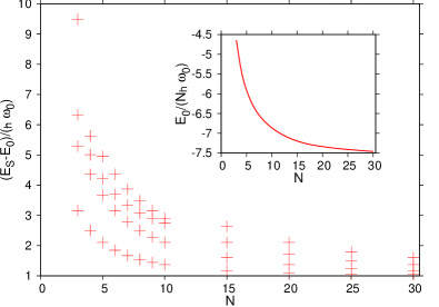
Figure 2: (Color online) Main plot: the excitation spectrum $E_{S}-E_{0}$ of the first four excited states of the inter-layer spectrum. Center-of-mass excitations are not included. Inset: Ground state $E_{0}/N$ as function of $N$ for $D=1$. The energy shift is included with $e_{12}=1$. Only nearest-neighbor layers interact with the same frequency, $\omega_{12}=3\omega_{0}$, all particles have equal mass, $m_{k}=m$. The energy unit is from the external trap frequency, $\hbar\omega_{0}$.

The inter-layer and center-of-mass solutions and related structures are now completely determined through eqs. (14) and (22), and for the total energy by use of eq. (38) as well. The resulting frequencies depend on $N$, as described in Section II.3. The total energy per layer decreases for small $N$ and saturate for large $N$ at constant values which increase with excitation energy in accordance with the individual frequencies in eq. (23). This saturation is closely related to the assumption of nearest neighbor inter-layer interaction. A longer-range interaction acting between layers further apart would lead to more than a linear $N$-dependence of the inter-layer energy. The additional increase would come from the normal mode frequencies in eq. (23) which would depend on a higher than linear power of $N$.

The excitation energies of the lowest excited states are shown in fig. 2 along with the evolution of the ground state energies including the zero-point shift, eq. (38) with $e_{12}=1$, with particle number in the inset. As the system gets larger, excitations become lower in energy and eventually approach the external field frequency. This lowering of the excitation energies with chain length is similar to acoustic phonons in solids arms-dip12 . The ground state energy also decreases with each additional layer, as each additional layer creates an additional interior layer which has eight attractive interactions with its neighbors. The quantity $E/N$ approaches a constant at large $N$ since the main contribution to the energy is linear in $N$. These plots are the same in 1, 2, and $3D$, if the interaction is isotropic (except for degeneracies). The increase in zero-point energy in higher dimensions is cancelled by the $D$-dependence of the shift in eq. (38).

IV.2 Inverse distance square potential

The remaining part of the problem is related to the two-body intra-layer Hamiltonian in eqs. (13) or (27). The fundamental frequency, $\omega$, is given by eq. (28). The intra-layer energy spectrum is given by eq. (29) for each of the $N$ layers.

The parameters of this part of the decoupled motion are layer number, $N$, dimension, $D$, and strength, $g$, of the $1/x^{2}$ potential. The latter two only enter through $l_{\textrm{eff}}$, which equals $l_{\textrm{eff}}=\sqrt{g+1/4}-1/2$ and $l_{\textrm{eff}}=\sqrt{g}-1/2$ for $s$-waves in $D=1$ and $2$, respectively. Thus the dimension dependence is very weak and for small $g$ only changing from $l_{\textrm{eff}}=0$ to $-1/2$. The number of layers only appears in the frequency obtained from eq. (28), but when only nearest neighbors interact, this frequency becomes independent of the total number of layers.

The energy spectrum is then obtained by adding four spectra, that is the inter-layer contribution shown in fig. 2, the $N-2$ times degenerate intra-layer spectrum from the inner layers, the $2$ identical end-layer spectra, and the total center-of-mass oscillator energies. The intra-layer contributions are $N$-independent except for the degeneracies. The $g$-dependence is entirely from the intra-layer summation, where for large $g$ it approximately amounts to a shift, $\hbar\omega\sqrt{g}$, of all the intra-layer energies.

If we also for $D=2$ include non-zero values of $l_{2}$, a large number of other energies appears through the value of $l_{\textrm{eff}}$. This would for special values of $g$ corresponding to integers give rise to precise degeneracies rather than just larger density of states. The $N$-dependence receives contributions from all parts of the Hamiltonian. The sum over all intra-layer energies is (at least for large $N$) essentially proportional to $N$. For large $N$ the inter-layer energy dependence in fig. 2 is proportional to $N$, and therefore comparable to the other contributing terms. The intra-layer excitations are higher in energy than the inter-layer string excitations. At the largest $N$ values, the intra-layer excitations approach the highest energy inter-layer excitation.

The spatial extension of the system is to a large extent determined by the intra-layer two-body structure characterized by the mean square radius. These radii are given by the expression in eq. (31) by insertion of the appropriate parameter values. These harmonic oscillator sizes are first of all determined by the length parameter, $b_{\omega}\propto 1/\sqrt{\omega_{k}}$, derived from eq. (28). The value of $\omega_{k}^{2}$ in eq. (28) increases from the outer to inner layers by about a factor of $2$ for large $\omega_{12}/\omega_{0}$. These sizes are almost independent of dimension which only enters weakly through $l_{\textrm{eff}}$.

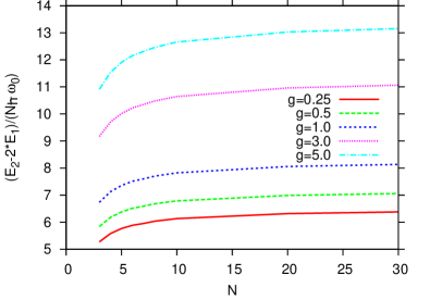
Figure 3: (Color online) The $D=1$ energies of double occupancy minus twice the energy of singly occupied layers as function of layer number $N$ for several strengths, $g$, of the $1/x^{2}$ potential. The parameters are the same as in fig. 2. We have not included the shift per layer, $-(e_{ik}+1)\hbar\omega_{12}(1-1/N)$, arising from the two-body binding energy.

The total energies are only useful in comparison with other energies. We may view the structure as two vertical strings interacting with each other through the direct intra-layer two-body repulsion and indirectly through the effective intra-layer potential arising from the interaction between particles in different strings. Then we can investigate string-string properties where the relative binding energy must be a crucial quantity. We must first decide a value for $V^{(shift)}$ to enter in both double and single string structures. The difference between zero-point shifts for these structures becomes $\delta V^{(shift)}=-D(N-1)(e_{12}+1)\hbar\omega_{12}$.

We show in fig. 3 the difference per layer between the combined double string system and two separated strings as function of the number of layers for different repulsive strengths. The structure of this energy difference can be divided into different contributions, that is (i) inter-layer difference of doubly occupied layers minus two times singly occupied layers, (ii) intra-layer contribution which is almost $D$ and $N$-independent but contains all the $g$ dependence, (iii) inter-layer center-of-mass energy difference between the two types of occupancy which is comparably small as arising from only one (vector) degree of freedom.

The energy difference in fig. 3 always increases with $N$ although approaching a constant depending on $g$ for large $N$. The inter-layer leading order coefficients on $N$ must be more than twice as large for two as it is for one string with singly occupied layers. The next to leading order vanishes after division by $N$ and the energy difference saturates at constant asymptotic values reached within about 10% when $N\simeq 10$.

The shifts are not included in fig. 3 since they strongly depend on which inter-layer interaction we are trying to simulate. With a shift corresponding to $e_{ik}=0$, $\delta V^{(shift)}/N\approx-3\hbar\omega_{0}$, the double string is never bound for any value of $N$. This is not surprising since two particles in different layers then have zero binding and therefore cannot supply any binding to the total system. If the two-body binding is given by $e_{12}=2$ all $1D$ curves in fig. 3 should be translated $9$ units downwards. Then any number of layers are bound as long as $g$ is less than about $1$.

The $2D$ results are qualitatively very similar. They also increase and approach constants as function of $N$ with increasing values as function of $g$. The chief difference is that the $2D$ energies are about 1.5 units of energy less than the corresponding $1D$ energy. This occurs because the effective $g$ value is always less for $2D$ (see the discussion following eq. (29)), so the $2D$ chain is experiencing a weaker repulsion than the $1D$ system. This weaker repulsion means that the larger zero-point shifts in $2D$ make the string-binding energy smaller in $2D$.

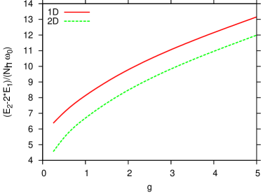
Figure 4: (Color online) The same energy differences as in fig. 3 for $N=30$, with the same parameters, but as function of the strength, $g$, of the $1/x^{2}$ potential for both $D=1$ and $D=2$.

The stability of a double string against two separate strings must obviously depend on the amount of repulsion between the strings. This arises entirely from the intra-layer $g$-dependence in the double string energy. We show the results for both $D=1$ and $D=2$ in fig. 4 as function of $g$ for a large value of $N(=30)$ where the asymptotic region is reached as seen in fig. 3. The inaccurately determined shift energy is again not included but for $\omega_{12}=3\omega_{0}$ the shift amounts to about $-3,-6,-9$ for $D=1$ for $e_{ik}=0,1,2$, respectively, and twice these amounts for $D=2$. It is then easy to see at which $g$-value a large number of layers become unstable. For fewer than $30$ layers the stability reaches to larger values of $g$.

These results are almost totally independent of $\omega_{12}$ since all energies for large $\omega_{12}/\omega_{0}$ are proportional to $\omega_{12}$. This includes the zero-point energies and the critical strength, $g_{crit}$, where the separation energies are zero, therefore remains the same. Instability then occurs for the same repulsion, $g$, and the same number of layers, $N$, for all large inter-layer interaction frequencies, $\omega_{12}$. On the other hand, the value of $e_{12}$ is crucial for the actual estimates.

The $D=2$ results are again qualitatively very similar. The separation energies also increase with increasing values of $g$. The string separation energies in figs. 3 and 4 are about $2$ energy units larger for $D=1$ than for $D=2$, that is for this choice of $\omega_{12}=3\omega_{0}$. The reasoning here is the same as for the previous plot, that is the centrifugal barrier present for $D=2$ effectively lowers the value of $g$. The energy is dependent on the square root of $g$, and that dependence is seen in the shape of the curves in figure 4.

IV.3 Delta-function intra-layer potential

The intra-layer extreme short-range repulsion has properties differing from the long-range $1/x^{2}$ potential. We calculate again spectra, two-body in-layer radii, and string separation energies. The total spectrum has precisely the same inter-layer contribution as shown in fig. 2. The center-of-mass term is trivially also the same. The differences in the total spectrum are therefore contained in the $N$ different intra-layer energies.

We therefore consider the energy expressions given in eqs. (33) and (37) corresponding to $D=1,2$, respectively. The dependence on the parameters clearly only arise from the energy unit, $\hbar\omega_{k}$, and $n_{\textrm{eff}}$. The frequency, $\omega_{k}$, is given by eq. (28) with the corresponding $N$ and $\omega_{12}$ dependence. The quantum number, $n_{\textrm{eff}}$, only depends on the ratio between scattering length and the derived oscillator length, $b_{\omega}$. These spectra in both $D=1$ and $D=2$ are discussed in busc98 ; liu10 . The oscillator sequence of excited states appears for all values of this ratio, while integer and half integer values of the principal quantum number result for large and small scattering lengths, respectively.

The difference to our application is only that the length unit is $b_{\omega}$ instead of the trap length defined in eq (28). This changes the scattering lengths in these units to much smaller values, and the asymptotic spectra are therefore reached for much smaller $a_{D}/b_{\omega}$-values.

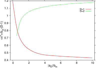
Figure 5: (Color online) The $D=1$ and $D=2$ mean square radii $\langle x^{2}\rangle/b^{2}_{\omega}-(D-1)$, of doubly occupied layers as function of strength, $a_{D}/b_{\omega}$, for a delta-function intra-layer interaction. The other interaction parameters are the same as specified in fig. 2. The larger sizes for $D=2$ is accounted for by the shift of $(D-1)$.

The intra-layer mean square radii in units of $b_{\omega}$ are necessarily determined by the ratio $a_{D}/b_{\omega}$. The resulting universal curves are shown in fig. 5 for the ground and lowest excited states states in both $D=1$ and $D=2$. The decreasing behavior for $D=1$ reflects the decreasing repulsion, with the opposite behavior for $D=2$ where the repulsion increases with increasing scattering length.

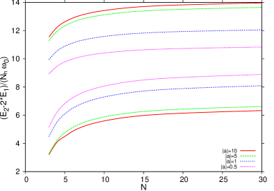
Figure 6: (Color online) The same energy differences as in fig. 3 for $D=2$ (largest values) and $D=1$ (smallest values) for a delta-function intra-layer interaction and several strengths given in terms of scattering lengths, $a_{D}/b_{\omega}$.

The separation energy between two coupled strings is again calculated for the delta-function repulsion. We show the results for $D=1$ and $D=2$ in fig. 6 as function of layer number, $N$, for different scattering lengths. As for the $1/x^{2}$ potential, we find the same behavior of an increase towards a constant large-$N$ value. This asymptotic energy also increases with the repulsive strength. We have still to translate the energy scale by the shift value in order to find critical $N$-values for given repulsion. The results for $D=1$ and $D=2$ are qualitatively similar, although with the order reversed as increasing repulsion is in opposite directions of changing scattering lengths.

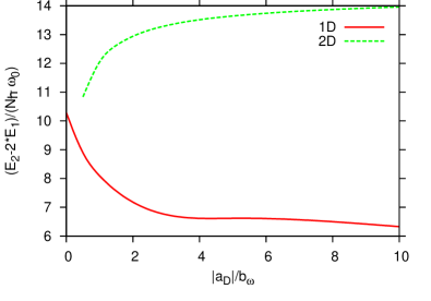
Figure 7: (Color online) The same energy differences as in fig. 4 for $N=30$ for a delta-function intra-layer interaction shown as functions of the strength in terms of the scattering lengths, $a_{D}/b_{\omega}$. Both $D=1$ (full, red) and $D=2$ (dashed, green) are shown.

The stability of a double string against two separate strings can be extracted from fig. 7. The separation energy is shown as function of decreasing repulsion for $N=30$ where the asymptotic region is reached as seen in fig. 6. This dependence arise entirely from the intra-layer $a$-dependence in the double string energy. The two-body intra-layer energies reach asymptotic values for extreme scattering lengths, which causes the many-body energies to also flatten out. The other contributions, including the energy shift, are independent of the two-body repulsion and discussed in connection with the $1/x^{2}$ potential. Again, instability therefore occurs for the same repulsion, $a_{D}/b_{\omega}$, and the same number of layers, $N$, for all large inter-layer interaction frequencies, $\omega_{12}$. The energies move in opposite directions between $D=1$ and $D=2$ given the opposite dependence of repulsive strength and scattering length magnitude in the different dimensions.

The scattering length dependent intra-layer excitation energies for the delta-function potential are, like in the case of the $1/x^{2}$ potential, mostly higher than the string excitations. However, in the case of a long string in $D=1$, some of the highest string excitations become higher in energy than the lowest intra-layer excitation. To give a sense of scale, the highest string excitation approaches $6.08$ $\hbar\omega_{0}$ when $\omega_{12}=3\omega_{0}$. For a range of scattering lengths, the lowest intra layer excitation is around $5.90$ $\hbar\omega_{0}$. This excitation occurs in the outermost layers, the interior layers’ excitations are all higher than the string excitations (coming in around 8.14 $\hbar\omega_{0}$). In two dimensions, the intra layer excitations are higher such that none of them are lower than a string excitation, even for very long strings.

V Summary and conclusion

We have formulated a prescription for a tremendous reduction of certain $2N$-body problems to an $N$-body oscillator problem and $N$ two-body problems. The conditions are rather severe but at least fulfilled for a number of experimentally relevant one and two-dimensional systems. The method is valid for a group of particles which can be separated topologically in $N$ groups (layers or tubes or other separable structures), each containing at most two arbitrarily interacting particles. All other one- and two-body interactions must be modelled by harmonic oscillator potentials.

The reduction of a theoretical problem to many two-body problems is an enormous simplification. The Schrödinger equation for nearly any interaction can be solved for two particles at least numerically, and other observables such as momentum distributions are easily calculated. If these two-body spectra are calculated, then statistical and thermodynamic quantities are also easily obtained, since the statistical properties of oscillators are also well known.

Decoupling of the many degrees-of-freedom is only achieved for equal masses of the two particles in each group. Different masses are allowed for different groups. Furthermore, two averages of the squares of specific oscillator frequencies must be equal. These interactions are related to the four interactions between pairs of particles in two groups. If one group only contains one particle it is allowed to have an arbitrary mass, and the identical averages still hold by insertion of zero interactions related to the removed particles.

Thus, we have one frequency constraint among four freqencies, where the most natural solution is that all these interactions are equal. We emphasize that this amounts to two conditions, that is equal masses in each group, and equal interactions between two groups, but both masses and interactions are allowed to vary between groups and pairs of groups. The result of these assumptions is total decoupling of degrees-of-freedom describing the relative oscillator motion between the center-of-masses of the groups, motion of the pairs in each layer, and the total center-of-mass motion within the external field. The $(2N)$-body problem is then reduced to an analytic $N$-body oscillator problem, $N$ independent two-body problems, and one center-of-mass analytic oscillator problem.

We illustrate how to apply the method by calculation of a number of basic properties in both one and two spatial dimensions. We choose two analytically solvable intra-group repulsive interactions where one is the long-range inverse distance squared potential and the other is the extreme short-range delta-function. We first specify pertinent analytic properties of these interactions.

Then we collect the variables describing our system, that is, individual masses, the number of particles, the intra-group repulsive strength, one-body external oscillator frequency, inter-group frequency and related shift of this oscillator potential. In the calculations we choose as few parameters as possible while retaining a number of fairly realistic features. All masses and one-body potentials are equal which leave dependence on them in the simple scaling through a choice of length and energy units. The inter-group frequencies are chosen to be identical for all particles in topologically neighboring groups and zero for all other inter-group potentials.

We are left with one inter-group frequency, the intra-group repulsive strengths, and the number of groups (layers or tubes). We first discuss the inter-group spectrum depending on $N$ and inter-group interaction frequency. We show the saturation of these energies per particle reached for large $N$ at values increasing linearly with inter-group frequency. The intra-group spectra are independent of $N$ for large $N$ and exactly given as function of repulsive strength in the effective intra-group oscillator units arising by combination of external trap and inter-group frequencies. All other intra-group properties, like root mean square radii, also only depend on the strength in such units.

The inverse distance squared potential has very small dimensional dependence. The delta-function potential, characterized by scattering length, $a_{D}$, leads superficially to very different behavior for $D=1$ and $D=2$, since positive and increasing $a_{1}$ corresponds to decreasing repulsion while the opposite is true for $a_{2}$ in two dimensions.

The total energy is calculated as the sum of all three (inter, intra and CM) parts. We calculate the total energy difference between doubly occupied groups and two times singly occupied groups. This energy is then the separation energy for this double string structure into two single strings. For both intra-group repulsive interactions and for both $D=1$ and $D=2$ we find that this energy difference saturates at constant values for large $N$. We calculate the saturation values as function of the repulsive strengths.

We can then in principle predict whether these structures are stable against string separation. For this we need to insert the energy gained by two interacting particles in different groups. This energy shift would depend strongly on the initial two-body interaction, unspecified in the present paper. We estimate a range of values and provide crude estimates of critical group number for stability for different repulsion and different dimensions.

In summary, we have discussed a versatile tool to calculate approximately a number of properties of structures separated topologically in groups with at most two particles in each. We demonstrate the capacity of the method by computing various energies as function of the variables describing the system, that is group number, spatial dimension, and intra- and inter-group one- and two-body interactions. A number of practically appearring systems can now be realistically approximated and investigated, that is for example dipolar particles in layer and tube structures. In the case of multiple layers, this was considered within a purely harmonic approach for chains with two or more particles per layer both at zero arms-dip12 and finite temperature arms-dip13 . In those studies the intralayer interaction was harmonic and modelling repulsive intralayer forces is therefore a delicate matter arms-dip12 . In comparison, the model present in the present paper allows for different choices of the intralayer interaction other than harmonic. In particular, for two chains per layer one may include the $1/r^{3}$ intralayer repulsion that dipoles have when their dipoles moments are polarized perpendicular to the layer, and thus investigate the chain-chain dynamics. This is an interesting topic for future study.

This work is supported by the Danish Council for Independent Research DFF Natural Sciences and the DFF Sapere Aude program.

References

- (1) I. Bloch, J. Dalibard and W. Zwerger, Rev. Mod. Phys 80, 885 (2008).
- (2) W. Heisenberg, Z. Physik 38, 411 (1926).
- (3) M. Goeppert-Mayer and J. H. D. Jensen. Elementary Theory of Nuclear Shell Structure John Wiley & Son, Inc., New York (1955).
- (4) M. Moshinsky, Am. J. Phys. 36, 52 (1968), Erratum: Am. J. Phys. 36, 763 (1968).
- (5) M. Moshinsky, N. Méndez, and E. Murow, Ann. Phys. 163, 1 (1985).
- (6) C. Amovilli and N. H. March, Phys. Rev. A 67, 022509 (2003).
- (7) C. Schilling, Phys. Rev. A 88, 042105 (2013).
- (8) N. R. Kestner and O. Sinanoglu, Phys. Rev. 128, 2687 (1962).
- (9) M. Taut, Phys. Rev. A 48, 3561 (1993).
- (10) X. Lopez, J. M. Ugalde and E. V. Ludeña, Eur. Phys. J. D 37, 351 (2006).
- (11) X. Lopez, J. M. Ugalde, L. Echevarría and E. V. Ludeña, Phys. Rev. A 74, 042504 (2006).
- (12) H. G. Laguna and R. P. Sagar, Phys. Rev. A 84, 012502 (2011).
- (13) C. Amovilli and N. H. March, Phys. Rev. A 69, 054302 (2004).
- (14) C. L. Benavides-Riveros and J. Várilly, Eur. Phys. J. D 66, 274 (2012).
- (15) J. Pipek and I. Nagy, Phys. Rev. A 79, 052501 (2009).
- (16) R. J. Yáñez, A. R. Plastino, and J. S. Dehesa, Eur. Phys. J. D 56, 141 (2010).
- (17) P. A. Bouvrie, A. P. Majtey, A. R. Plastino, P. Sánchez-Moreno, and J. S. Dehesa, Eur. Phys. J. D 66, 1 (2012).
- (18) C. L. Benavides-Riveros, J. M. Gracia-Bondía, and J. C. Várilly, Phys. Rev. A 86, 022525 (2012).
- (19) P. Kościk and A. Okopińska, Few-Body Syst. 54, 1637 (2013).
- (20) C. L. Benavides-Riveros, I. V. Toranzo, and J. S. Dehesa, J. Phys. B:At. Mol. Opt. Phys. 47, 195503 (2014).
- (21) P. A. Bouvrie, A. P. Majtey, M. C. Tichy, J. S. Dehesa, and A. R. Plastino, Eur. Phys. J. D 68, 346 (2014).
- (22) N. F. Johnson and M. C. Payne, Phys. Rev. Lett. 67, 1157 (1991).
- (23) Z. Wang, A. Wang, Y. Yang, and X. Li, Commum. Theor. Phys. 58, 639 (2012).
- (24) C. Schilling, D. Gross, and M. Christandl, Phys. Rev. Lett. 110, 040404 (2013).
- (25) L. Bombelli, R. K. Koul, J. Lee, and R. D. Sorkin, Phys. Rev. D 34, 373 (1986).
- (26) M. Srednicki, Phys. Rev. Lett. 71, 666 (1993).
- (27) J. Eisert, M. Cramer, and M. B. Plenio, Rev. Mod. Phys. 82, 277 (2010).
- (28) F. Brosens, J. T. Devreese, and L. F. Lemmens, Phys. Rev. E 55, 227 (1997); 55, 6795 (1997); 57, 3871 (1998); 58, 1634 (1998).
- (29) M. A. Załuska-Kotur, M. Gajda, A. Orłowski and J. Mostowski, Phys. Rev. A 61, 033613 (2000).
- (30) J. Yan, J. Stat. Phys. 113, 623 (2003).
- (31) M. Gajda, Phys. Rev. A 73, 023693 (2006).
- (32) J. Tempere, F. Brosens, L. F. Lemmens, and J. T. Devreese, Phys. Rev. A 58, 3180 (1998); ibid. 61, 043605 (2000); ibid 61, 043605 (2000).
- (33) J. R. Armstrong, N. T. Zinner, D. V. Fedorov, and A. S. Jensen, J. Phys. B:At. Mol. Opt. Phys. 44, 055303 (2011).
- (34) J. R. Armstrong, N. T. Zinner, D. V. Fedorov, and A. S. Jensen, Physica Scripta T151, 014061 (2012).
- (35) J. R. Armstrong, N. T. Zinner, D. V. Fedorov, and A. S. Jensen, Phys. Rev. E 85, 021117 (2012).
- (36) J. R. Armstrong, N. T. Zinner, D. V. Fedorov, and A. S. Jensen, Phys. Rev. E 86 , 021115 (2012).
- (37) T. Lahaye, C. Menotti, L. Santos, M. Lewenstein, and T. Pfau, Rep. Prog. Phys. 72, 126401 (2009).
- (38) L. D. Carr, D. DeMille, R. V. Krems, and J. Ye, New J. Phys. 11, 055049 (2009).
- (39) M. A. Baranov, Phys. Rep. 464, 71 (2008).
- (40) M. H. G. Miranda et al., Nature Phys. 7, 502 (2011).
- (41) D. W. Wang, E. Demler, and M. D. Lukin, Phys. Rev. Lett. 97, 180143 (2006).
- (42) J. R. Armstrong, N. T. Zinner, D. V. Fedorov, and A. S. Jensen, Eur. Phys. J. D 66, 85 (2012).
- (43) B. Capogrosso-Sansone and A. Kuklov, J. Low Temp. Phys. 156, 213 (2011).
- (44) J. R. Armstrong, N. T. Zinner, D. V. Fedorov, and A. S. Jensen, Few-Body Syst. 54, 605 (2013).
- (45) M. Klawunn, J. Duhme, and L. Santos, Phys. Rev. A 81, 013604 (2010).
- (46) A. G. Volosniev et al., New J. Phys. 15, 043046 (2013).
- (47) J. Karwowski and L. Cyrnek, Annalen der Physik 13, 181 (2004).
- (48) J. Karwowski, Int. J. Quan. Chem. 108, 2253 (2008).
- (49) J. Karwowski and K. Szewc, J. Phys.: Conf. Ser. 213, 012016 (2010).
- (50) D. Manzano, A. R. Plestino, J. S. Dehesa, and T. Koga, J. Phys. A: Math. Theor. 43, 275301 (2010).
- (51) R. Crandell, R. Whitnell, and R. Bettega, Am. J. Phys. 52, 438 (1984).
- (52) F. Calogero, J. Math. Phys. 10, 2191 (1969).
- (53) F. Calogero, J. Math. Phys. 12, 419 (1971).
- (54) T. Busch, B.-G. Englert, K. Rza̧żewski, and M. Wilkens, Found. Phys. 28, 549 (1998).
- (55) X.-J. Liu, H. Hu, and P. D. Drummond, Phys. Rev. B 82, 054524 (2010).
- (56) M. Abramowitz and I.R. Stegun: Handbook of mathematical functions (Dover publications, Inc., New York 1970).