Relativistic Bessel Cylinders

Abstract

A set of cylindrical solutions to Einstein’s field equations for power law densities is described. The solutions have a Bessel function contribution to the metric. For matter cylinders regular on axis, the first two solutions are the constant density Gott-Hiscock string and a cylinder with a metric Airy function. All members of this family have the Vilenkin limit to their mass per length. Some examples of Bessel shells and Bessel motion are given.

I Introduction

Exact solutions in cylindrical spacetimes have found a wide variety of applications in general relativity SKM+03 . The 1917 solutions of Weyl and Levi-Civita are used for cylindrical vacuums BM91 ; WSS97 ; L-B14 , and there are a wide range of cylindrical matter solutions. Krasinski Kra93 has reviewed many of the cylindrical solutions with perfect and imperfect fluid sources. Other fluid descriptions include the 1937 van Stockum rotating dust solution v-Sto37 , constant density string solutions His85 ; Got85 , cylinders with a cosmological vacuum Lin86 , and global solutions for static cylinders BLS+04 . There is interest in cylindrical shells Sta84 ; BZ02 , both static and rotating KLB11 . Solutions have been combined to create van Stockum cylinders with Gott-Hiscock cores Kri03 or matter cylinders with vacuum cores SY12 . While infinite cylinders are not physically realized, cylindrical structures can be used to investigate some gravitational models BK13 and can be physically relevant for systems with cylindrical waves Bic00 , or cosmic strings CV87 ; MMT+10 and have recently become of interest BKL13 ; Ric13 ; BS14 in wormhole applications.

In this paper we examine the static cylindrical field equations for the following metric

$$ds^{2}=-dt^{2}+dr^{2}+F^{2}d\varphi^{2}+dz^{2},\text{ \ \ }F=F(r).$$ (1)

We assume power law matter densities, and it emerges that for such densities the field equations can be cast into a form which has solutions obeying a Bessel equation. The solutions are characterized by the Bessel index or the power law exponent. For integer power laws, two members of the matter filled cylinder family are (a) the Gott-Hiscock His85 ; Got85 constant density solution and (b) a solution with linear density and metric function $F(r)$ as a combination of Airy functions. All interior solutions are matched to an exterior vacuum Levi-Civita metric with angular deficit factor $"\alpha"$.

$$ds^{2}=-dt^{2}+d\rho^{2}+dz^{2}+\alpha^{2}\rho^{2}d\varphi^{2}$$ (2)

Bessel shells, matched to a central Levi-Civita vacuum are also discussed and examples of Bessel motions are given. In the next section we develop the field equations deriving from metric (1), and give several examples of the solutions for both full matter cylinders and shells. Among the recurring questions about cylindrical solutions is the limit of mass per length FG88 ; BLS+04 . We show that the linear mass density of the solutions have the Vilenkin limit Vil81 and compare the possible cylinder size limits by using the zeros of the angular deficit factor $"\alpha".$ Several ways of adding Bessel functions to the matter motion are discussed in the third part of the paper.

II The Solution Family

Field Equations

For the metric of Eq.(1), the interior field equations are (with primes denoting $\partial/\partial r$ and units such that $G=c=1$)

$$G_{tt}=-G_{zz}=-\frac{F^{\prime\prime}}{F}=8\pi\varepsilon.$$ (3)

The desired Bessel form PZ95 ; AS72 is

$$\frac{F^{\prime\prime}}{F}+\frac{a}{r}\frac{F^{\prime}}{F}+br^{n-2}=0.$$ (4)

For simplicity, we choose $a=0$. The Bessel equation is

$$\frac{F^{\prime\prime}}{F}+br^{n-2}=0.$$ (5)

where the density in Eq.(3) was chosen as $8\pi\varepsilon=br^{n-2}$, so that the field equation is a Bessel equation. The energy density is either constant or zero on axis for $n\geq 2.$ The $n=2$ constant density cylinder will be used as a reference solution. Defining the $n=2$ density as $\varepsilon_{0}$, the power law energy density is

$$\varepsilon=\varepsilon_{0}(r/r_{0})^{n-2},$$ (6)

with $\ b=8\pi\varepsilon_{0}/r_{0}^{n-2}.$ The Bessel solution for the metric function PZ95 ; AS72 is

$$F(r)=\sqrt{r}\left[A_{0}J_{1/n}(\frac{2\sqrt{b}\text{ }r^{n/2}}{n})+B_{0}Y_{1/n}(\frac{2\sqrt{b}\text{ }r^{n/2}}{n})\right].$$ (7)

The Kretchmann scalar for metric (1) is

$$R^{\alpha\beta\mu\nu}R_{\alpha\beta\mu\nu}=(2\frac{F^{\prime\prime}}{F})^{2}=4b^{2}r^{2(n-2)}.$$ (8)

When $n<2$ the energy density and Kretchmann scalar are singular on the axis. For $n=2$ the curvature is constant.

Bessel functions are most easily described with a coordinate argument $J_{1/n}(x)$. For the Bessel cylinders $x:=C(n)r^{n/2},$ with $C(n):=2b^{1/2}/n$ and

$$F=\left[\frac{x}{C(n)}\right]^{1/n}[A_{0}J_{1/n}(x)+B_{0}Y_{1/n}(x)].$$ (9)

Herrera and Di Prisco HDiP12 have introduced a classification system for relativistic cylinders with a general metric $g^{\text{H-DiP}}=[-A^{2},$ $A^{2},$ $B^{2},$ $C^{2}]$. For static anisotropic matter distributions the solution depends on a set of three functions, $(Y_{k},Y_{s},E_{k}),$ related to the metric functions $(A,B,C)$. $Y_{k}$ and $Y_{s}$ depend on metric functions $A$ and $B$ which are zero for the Bessel cylinders. The structure scalar, $E_{k}=F^{\prime\prime}/2F$,  is determined by the energy density through the field equations. As expected, the other curvature functions (Weyl, Ricci, Ricci scalar) also depend on the same field relation and are proportional to the energy density. In the next section, we describe full matter cylinders with $n\geq 2,$ where the limited range of $n$ insures a non-singular axial density.

III Cylinder Properties

Matter Filled Cylinders: $n\geq 2$

For the special cylinders discussed here, the full matter cylinder has energy density and axial tension with $\varepsilon=-P_{z}.$ The normalization of $F(r)$ depends on the choice of axial behavior. With $n\geq 2,$ the axial density is either constant or zero. One can require that $F(r)$ approach the interior radial coordinate near the axis. $F(r)$ simplifies to the Bessel form

$$F(r)=A_{0}\sqrt{r}J_{1/n}[C(n)r^{n/2}].$$

To first order, the Bessel expansion OMS00 is

$$J_{1/n}[Cr^{n/2}]\text{ }{\LARGE\sim}\text{ }\frac{\sqrt{r}}{\Gamma(\frac{n+1}{n})}[\frac{C(n)}{2}]^{1/n}\ +\ ....$$ (10)

This determines the constant $A_{0}$. The $F(r)$ solution is

$$F(r)=\Gamma(\frac{n+1}{n})\left[\frac{2}{C(n)}\right]^{1/n}\sqrt{r}J_{1/n}[C(n)r^{n/2}],$$ (11)

or, in terms of the x-coordinate,

$$F(x)=\Gamma(\frac{n+1}{n})\left[\frac{2}{C(n)^{2}}\right]^{1/n}x^{1/n}J_{1/n}(x).$$ (12)

The angular deficit factor and interior-exterior coordinate map follow from the metric and extrinsic curvature match to vacuum Levi-Civita at $(r_{B}$, $\rho_{B}):$

$$\alpha =\frac{\partial F(x_{B})}{\partial r}=\Gamma(\frac{n+1}{n})J_{(1-n)/n}(x_{B})2^{1/n-1}[nx_{B}^{(n-1)/n}]$$ (13)

$$\rho_{B} =\frac{J_{1/n}(x_{B})}{J_{(1-n)/n}(x_{B})}\ \frac{2x_{B}^{(2-n)/n\ }}{nC(n)^{2/n}}.$$ (14)

In the ”Mass Density” section we show that the Bessel cylinders, in the $n\geq 2$ parameter range, have the Vilenkin upper limit on their mass per length, the limit occurring at $\alpha=0.$ For the simplest interiors, the zero of $J_{(1-n)/n}$ set an upper limit on $x_{B}$ (and $r_{B})$. In the following section we consider two examples in the range $n\geq 2:$ $n=2\$and $n=3.$

Matter Filled Cylinders: n = 2, 3

The $n=2$ solution is the Gott-Hiscock His85 ; Got85 string with constant density $\varepsilon=\varepsilon_{0}$, constant curvature, and axial tension. $n=3$ describes an Airy cylinder. For $n=2$, the $x$ coordinate is linearly related to $r:$ $x=kr$, with $k=\sqrt{8\pi\varepsilon_{0}}$. The metric function in terms of the density is

$$F(x)=\frac{\sqrt{2}}{k}\ \Gamma(\frac{3}{2})\ x^{1/2}J_{1/2}(x).$$ (15)

Using the relation between Bessel functions of half order and spherical Bessel functions identifies this as the Gott-Hiscock His85 ; Got85 constant density string solution.

$$F_{2}(x)=\frac{\sin(x)}{k},\text{ \ \ \ }\alpha=\cos(x_{B}),\text{ \ \ \ }\rho_{B}=\frac{\tan(x_{B})}{k}.$$ (16)

The $n=3$ string has a linear mass density $\varepsilon=\varepsilon_{0}(r/r_{0})$.  Here

$$x:=\frac{2}{3}kr_{0}(r/r_{0})^{3/2}.$$

The metric function $F,$ given in terms of the x-coordinate is

$$F(x)=\Gamma(\frac{4}{3})\left[\frac{2}{C^{2}(3)}\right]^{1/3}x^{1/3}J_{1/3}(x),\text{\ \ \ }C(3)=\frac{2k}{3\sqrt{r_{0}}}.$$ (17)

The Levi-Civita match gives the angular deficit and interior-exterior coordinate map

$$\alpha =\frac{3}{2}\Gamma(\frac{4}{3})J_{-2/3}(x_{B})(\frac{x_{B}}{2})^{2/3}$$ (18)

$$\rho_{B} =(\frac{k^{2}}{r_{0}})^{1/3}\frac{J_{1/3}(x_{B})}{J_{-2/3}(x_{B})}(\frac{2}{3x_{B}})^{1/3}.$$ (19)

For the $n=2$ solution, the $x$ and $r$ coordinates are linearly related. For $n=3$, the Bessel functions linear in $x$ are related to Airy functions with arguments $"\chi"$ linear in the r-coordinate.

$$J_{1/3}(x)=\sqrt{\frac{3}{4\chi}}\left[\sqrt{3}Ai(-\chi)-Bi(-\chi)\right],$$ (20)

with

$$x=(2/3)\chi^{3/2}=C(3)r^{3/2}.$$

The Airy functions do not simplify the analysis but provide a function linear in $r$. Their occurrence is interesting because they provide a text book example of a non-relativistic wave packet appearing as solutions to the Schrödinger equation with a linear potential BB79 . (In particular, the Schrödinger equation written with a linear potential is an Airy equation

$$\frac{d^{2}\psi}{dz^{2}}-z\psi=0.$$ (21)

This equation has solutions $Ai(z)$ for one of the two kinds of Airy functions.) Here the Airy functions are the $1-d$ envelope of the cylinder cross section and the linear behavior is in the density.

Mass Density

The mass per length is calculated as an integral over density.

$$M=\mu L={\textstyle\int\limits_{0}^{L}}dz{\textstyle\int\limits_{0}^{2\pi}}d\phi{\textstyle\int\limits_{0}^{r_{B}}}\varepsilon(r)F(r)dr,$$ (22)

with

$$\mu=2\pi\varepsilon_{0}\Gamma(\frac{n+1}{n})\ [\frac{2}{C(n)}]^{1/n}{\textstyle\int\limits_{0}^{r_{B}}}(\frac{r}{r_{0}})^{n-2}\sqrt{r}\ J_{1/n}[C(n)r^{n/2}]dr.$$

Changing variables, the linear density becomes

$$4\mu =n\Gamma(\frac{n+1}{n})2^{(1-n)/n}\ {\textstyle\int\limits_{0}^{x_{B}}}x^{(n-1)/n}\ J_{1/n}(x)dx$$ (23)

$$4\mu =1-\frac{\Gamma(1/n)}{2^{1-1/n}}x^{(n-1)/n}J_{(1-n)/n}(x).$$ (24)

Comparing to Eq.(18), the linear density is related to the deficit factor.

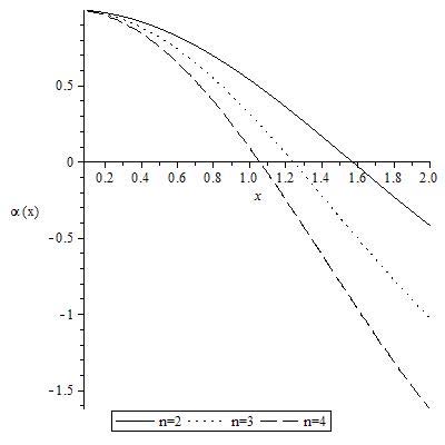
Figure 1: Angular deficit factor vs boundary position for $n=2,3,4$.

$$4\mu=1-\alpha.$$ (25)

This relation between the linear mass density and the angular deficit factor was originally predicted by Vilenkin Vil81 in a linear approximation. Futamase and Garfinkle FG88 pointed out that Eq.(25) is not in true in general, but seems to be obeyed for systems with small radial stress Isr77 . There is no radial stress in these solutions and it is valid for the Bessel cylinders. All of the $n\geq 2$ cylinders have the same upper limit, $\mu=1/4,$ on their linear mass density. The cylinders differ in the the boundary radius at which this upper limit occurs. Figure 1 shows the angular deficit factor as a function of $x$ for several $n$ values. As $n$ increases, the zeros of the angular deficit factor and the upper limit on $\mu$ occur at increasingly smaller values. The metric function $F(r)$ also has Bessel zeros, but the first zeros of the angular deficit occur at smaller values than the zeros of $F(r)$. Requiring $\alpha<1$ for positive linear density, the angular deficit sets the upper limit on the exterior boundary. If the string boundary is constrained to lie within the first zero, higher $n$ values can produce smaller objects.

Cylindrical Shells: n $<$ 2

Shell Description

Bessel shells, with no axial content, can cover the lower part of the $n$ range with a well behaved density. The general $F(x)$ is

$$F=\left[\frac{x}{C(n)}\right]^{1/n}[AJ_{1/n}(x)+BY_{1/n}(x)].$$

The shells will match to an interior Levi-Civita vacuum solution at $x_{1}$, with no angular deficit in the interior and to Levi-Civita solution with an angular deficit at $x_{2}$ in the exterior. The matching conditions are

$$[\frac{x_{1}}{C(n)}]^{1/n}[A_{0}J_{1/n}(x_{1})+B_{0}Y_{1/n}(x_{1})] =\rho_{1}$$ (26)

$$[\frac{x_{2}}{C(n)}]^{1/n}[A_{0}J_{1/n}(x_{2})+B_{0}Y_{1/n}(x_{2})] =\alpha\rho_{2}.$$ (27)

The extrinsic curvature match provides

$$[A_{0}J_{(1-n)/n}(x_{1})+B_{0}Y_{(1-n)/n}(x_{1})](\frac{n}{2})x_{1}^{(n-1)/n}C(n)^{1/n} =1$$ (28)

$$[A_{0}J_{(1-n)/n}(x_{2})+B_{0}Y_{(1-n)/n}(x_{2})](\frac{n}{2})x_{2}^{(n-1)/n}C(n)^{1/n} =\alpha.$$ (29)

The three possible cases are $A_{0}$ or $B_{0}$ zero or both non zero. $B_{0}=0$ creates shells that transition smoothly into the full matter cylinder. For $B_{0}=0$ the matching conditions set the value of $A_{0}$ in terms of the inner boundary, $x_{1}$, and the boundary parameters are

$$A_{0}=(\frac{2}{n})\frac{x_{1}^{(1-n)/n}}{J_{(1-n)/n}(x_{1})C(n)^{1/n}},\text{ \ \ }\alpha=\left[(\frac{x_{2}}{x_{1}})^{(n-1)/n}\right]\frac{J_{(1-n)/n}(x_{2})}{J_{(1-n)/n}(x_{1})},$$ (30)

with boundary locations $x_{i},$ $i=1,2.$

$$\rho_{i}=(\frac{2}{n})\left[\frac{x_{i}^{(2-n)/n}}{C(n)^{2/n}}\right]\frac{J_{1/n}(x_{i})}{J_{(1-n)/n}(x_{i})}.$$ (31)

The $A_{0}=0$ shell is a new solution. For this case we have

$$B_{0}=(\frac{2}{n})\frac{x_{1}^{(1-n)/n}}{Y_{(1-n)/n}(x_{1})C(n)^{1/n}},\text{ \ \ }\alpha=\left[(\frac{x_{2}}{x_{1}})^{(n-1)/n}\right]\frac{Y_{(1-n)/n}(x_{2})}{Y_{(1-n)/n}(x_{1})}.$$ (32)

The boundary locations are

$$\rho_{i}=(\frac{2}{n})\left[\frac{x_{i}^{(2-n)/n}}{C(n)^{2/n}}\right]\frac{Y_{1/n}(x_{i})}{Y_{(1-n)/n}(x_{i})}.$$ (33)

All choices obey the Vilenkin limit. There are differences in the position of the boundaries and in the angular deficit. The $n=1$ shell  is an interesting example that illustrates the differences. The angular deficits and boundary positions for $n=1$ shells are simple Bessel ratios.

$$B_{0}=0:\text{ \ }\rho_{i}=\frac{2x_{i}}{C(1)^{2}}\frac{J_{1}(x_{i})}{J_{0}(x_{i})},\text{ \ }\alpha=\frac{J_{0}(x_{2})}{J_{0}(x_{1})},$$ (34)

$$A_{0}=0:\text{ \ }\rho_{i}=\frac{2x_{i}}{C(1)^{2}}\frac{Y_{1}(x_{i})}{Y_{0}(x_{i})},\text{ \ }\alpha=\frac{Y_{0}(x_{2})}{Y_{0}(x_{1})}.$$ (35)

The interior and exterior boundary positions for a given choice of boundary $"x"$ are shown in Figure 2 where the possible smaller core radii for the $B_{0}=0$ shell are seen. From Figure 2, an exterior boundary value, $x_{2}=0.4$, was selected for both shells. Figure 3 shows the variation in the angular deficit as the interior boundary position changes. The $A_{0}=0$ shell has much larger angular deficits for small cores (thick shells). As the shells get thinner, with the inner core boundary moving away from axis, the singular axial behavior of $Y_{1/n}$ ceases to dominate and the deficit approaches one.  When the two boundaries coincide, $\alpha=1,$ then the mass per length is zero [see Eq.(25)] and the entire spacetime is vacuum Levi-Civita.

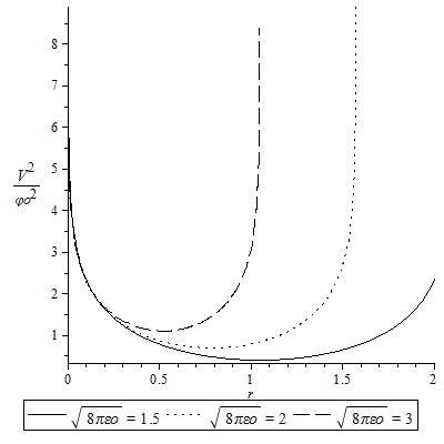
Figure 2: $V^{2}/\phi^{2}$ vs r for $n=2$and several density choices

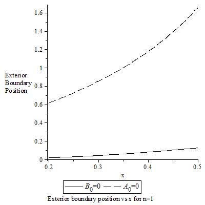
Figure 3: Boundary   vs boundary position $x$ for $n=1.$

IV Describing the Motion

Geodesics

In these models, although the matter in the cylinder is static, the geodesics contain interesting information about the cylinders and the boundary choices. In the interior, the $\phi$ geodesic provides angular momentum conservation:

$$\frac{d\phi}{d\tau}F^{2}=\phi_{0}.$$ (36)

Close to the axis, $F\sim r,$ and the equation is analogous to $\omega r^{2}=const$. The radial geodesic is

$$\frac{d^{2}r}{d\tau^{2}}=(\frac{F^{\prime}}{F})\phi_{0}^{2}.$$ (37)

Converting to radial derivatives we have

$$\frac{\dot{r}^{2}}{2}=\phi_{0}^{2}\ln F+const.$$ (38)

This can be written as

$$\frac{\dot{r}^{2}}{2}+V^{2}=const.$$ (39)

where $V^{2}$ is an effective potential Sch85 in the interior given by $V^{2}=-\phi_{0}^{2}\ln F$.

$$V^{2}=-\phi_{0}^{2}\ln\left[\Gamma(\frac{n+1}{n})[\frac{2}{C(n)^{2}}]^{1/n}x^{1/n}J_{1/n}(x)\right].$$ (40)

For example, with $n=2,$ $k=\sqrt{8\pi\varepsilon_{0}}$, and $x=kr$, we have $V^{2}=-\phi_{0}^{2}\ln(\frac{\sin(kr)}{k})$. The potential is concave upward with a stable equilibrium at $F^{\prime}=0$. The equilibrium is at a zero of $J_{-1.2}(kr)$, with the first zero occurring at $kr\sim 1.57.$ The shape of the potential suggests that the matter interior is stable under small radial perturbations with boundary chosen inside the potential.  The shape of the potential for $n=2$ and several density choices are shown in Figure 4, which illustrates that the choice of exterior boundary is not only dependent on the allowed boundary ranges but also on the potential shape.

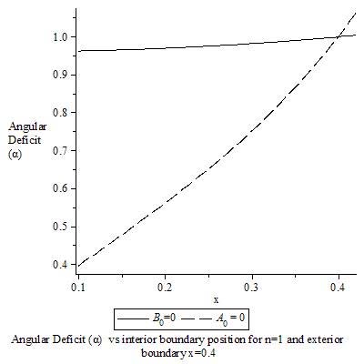
Figure 4: Angular deficit   vs x.

Motion with a Bessel Description

Bessel functions can be added to a fluid description by the choice of velocity profile. Two examples are considered. The first example looks at the conditions for an irrotational motion described by Bessel fuctions. In the second example, the geodesic description is used to add Bessel behavior to a radial velocity.

Tangential Motion

A 4-velocity with a rotational component $U^{i}=[U^{0},0,U^{\varphi},0]$ has vorticity in the z direction proportional to

$$\omega^{z}\sim\frac{\partial(U^{\varphi}F)}{\partial r}.$$ (41)

An irrotational motion will have $U^{\varphi}\sim c_{1}/F(r).$ Close to the axis, this is the $c_{1}/r$ velocity profile associated with classical point-vortex motion. For thick shells, near the outer boundary, the velocity profile, while still irrotational, is no longer that of a point vortex. The shells discussed here have Levi-Civita vacuum interiors. They would need a matter core to describe vortices, for example, of the Rankine type.

Radial Motion

Radial motion with a Bessel function description can be added by considering the geodesics of test particles. They involve a non-zero angular momentum parameter so the actual motion would include some rotational component. The radial geodesic equation can be written with an extra derivative as

$$\frac{d^{2}}{dr^{2}}(\frac{\dot{r}^{2}}{2})+\frac{d}{dr}(\frac{d\ln F}{dr})=0.$$ (42)

This is an Airy equation for $\dot{r}^{2}/2$ if the second term has the form

$$\frac{d}{dr}(\frac{d\ln F}{dr})=-r(\frac{\dot{r}^{2}}{2})=-r(\phi_{0}^{2}\ln F+const).$$ (43)

putting Airy function into the radial velocity. This example changes the metric function. Using the geodesic solution, this becomes a generating equation for a new $F(r)$:

$$F(r) =e^{[\lambda(r)-1]/\phi_{0}^{2}}$$ (44)

$$\frac{d}{dr}(\frac{d\ln F}{dr}) =-r(\phi_{0}^{2}\ln F+1)$$ (45)

$$\frac{d^{2}\lambda}{dr^{2}}+(\phi_{0}^{2})r\lambda =0.$$ (46)

This is a particular Bessel equation of order $1/3$. Again, there is Airy behavior in metric function $F(r)$, but now it appears exponentially with non-zero angular momentum parameter $\phi_{0}^{2}$.

V Discussion

A family of Bessel solutions of the Einstein equations with power law density $\varepsilon\sim r^{n-2}$, and axial stress were developed. For $n\geq 2$, the first two solutions are the $n=2$ Gott-Hiscock string and an $n=3$ Airy cylinder. All cylinders have the Vilenkin upper limit on their mass per length. The cylinders reach that limit at increasing smaller radii. The choice of power law density was motivated by recent experiments using lasers SC07 ; SBD+08 and electron beams BLL+13 that reported observational evidence for beam caustics described by Airy functions. Airy functions are normally associated with a linear potential in the Schrödinger equation. The Airy functions here are in the metric, and the linear dependence occurs for the $n=3$ density. The particular $n=3$ Airy solution discussed here is part of the Gott-Hiscock family, and there are other related solutions containing Airy functions.

Most of the Bessel cylinders described in this work are static but extensions to stationary or time dependent solutions for metrics containing Airy functions would also be of interest for some cylindrical beam applications. The cylinders studied here can have a fractional Bessel index, but are solutions of an integer derivative Bessel equation. Using the relation between the fractional derivative of the sine OMS00 and Bessel functions provides

$$J_{1/n}(\sqrt{z})=\frac{d^{(n-2)/2}}{d^{(n-2)/2}}\sin(\sqrt{z}).$$

Links to fractional calculus provide a possible direction for future work.

References

- (1) Exact Solutions of Einstein’s Field Equations, Eds. H. Stephani, D. Kramer, M. MacCallum, C. Hoenselaers and E. Herlt, 2nd Ed. (Cambridge University Press, Cambridge, U.K. 2003). Ch 22
- (2) W. Bonnor and M. Martins, Class. Quantum Grav. 8, 727 (1991). The interpretation of some static vacuum metrics
- (3) A. Wang, M. da Silva, and N. Santos, Class. Quantum Grav. 14, 2417 (1997). On parameters of the Levi-Civita solution
- (4) D. Lynden-Bell, The Torqued Cylinder and Levi-Civita’s metric. arXiv/gr-qc/1402.6171 (2014).
- (5) A. Krasinski, Physics in an Inhomogeneous Universe, (N. Copernicus Astronomical Center, Polish Academy of Sciences, Warsaw, Poland, 1993).
- (6) W.J. van Stockum, Proc. Roy. Soc. Edinburgh, 57, 135 (1937). Time loop outside a rotating cylinder
- (7) W.A. Hiscock, Phys. Rev. 31, 3288 (1985). Exact Gravitational Field of a String
- (8) J.R.Gott III, Astrophys. J. 288, 422 (1985). Gravitational Lensing Effects of Vacuum Strings: Exact Solutions
- (9) B. Linet, J. Math. Phys. 27, 1817 (1986). The static, cylindrically symmetric strings in general relativity with cosmological constant
- (10) J. Bicak, T. Ledvinka, B.G. Schmidt, and M. Zofka, Class. Quantum Grav. 21, 1583,(2004). Static fluid cylinders and their fields: global solutions
- (11) J. Stachel, J. Math. Phys. 25, 338 (1984). The gravitational fields of some rotating and nonrotating cylindrical shells of matter
- (12) J. Bicak and M. Zofka, Class. Quantum Grav. 19, 3653 (2002). Notes on static cylindrical shells
- (13) J. Katz, D. Lynden-Bell, J. Bicak, Class. Quantum Grav. 28, 065004 (2011). Centrifugal force induced by relativistically rotating spheroids and cylinders.
- (14) J.P. Krisch, Class. Quantum Grav. 20, 1605 (2003). Cosmic string in the van Stockum cylinder
- (15) M. Sharif and Z. Yousaf, Can. J. Phys. 90, 865 (2012). Expansion-free Cylindrically Symmetric Models
- (16) D. Lynden-Bell and J. Katz, Thought Experiments on Gravitational Forces, arXiv:/astro-ph/1312.6043
- (17) J. Bicak, Selected solutions of Einstein’s field equations: their role in general relativity and astrophysics, arXiv/gr-qc/0004016 (2000).
- (18) J. Carriga and E. Vergaguer, Phys. Rev. D 36, 2250 (1987). Cosmic strings and Einstein-Rosen soliton waves
- (19) E. Morganson, P. Marshall, T. Treu, T. Schrabback, and R.D. Blandford, Mon. Not. Roy. Astron. Soc. 406, 3452 (2010). Direct Observation of cosmic strings via their strong gravitational lensing effect-II. Results from the HST/ACS image archive
- (20) K.A. Bronnikov, V.G. Krechet, and J.P.S. Lemos, Phys. Rev. D 87, 084060 (2013). Rotating cylindrical wormholes
- (21) M.G. Richarte, Phys. Rev. D 88, 027507 (2013). Cylindrical wormholes with positive cosmological constant
- (22) K.A. Bronniov and M.V. Skvortsova, Cylindrically and axially symmetric wormholes. Throats in vacuum, arXiv/gr-qc/1404.5750 (2014).
- (23) T. Futamase and D.Garfinkle, Phys. Rev. D 37, 2086 (1988). What is the relation between and for a cosmic string?
- (24) A. Vilenkin, Phys. Rev. D 23, 852 (1981). Gravitational Field of Vacuum Domain Walls and String
- (25) A.D. Polyanin and V.F. Zaitsev, Exact Solutions for Ordinary Differential Equations (CRC Press, Boca Raton, FL, 1995) p. 147.
- (26) M. Abromowitz and I.S. Stegun, Handbook of Mathematical Functions (Dover Publications, New York, 1972). p 446
- (27) L. Herrera and A. Di Prisco, Gen. Rel. Gravit. 44, 2645 (2012). Cylindrically Symmetric Relativistic Fluids: A study based on Structure Scalars
- (28) K. Oldham, J. Myland, and J. Spanier, An Atlas of Functions (Springer Verlag, Berlin, 2000). p.556.
- (29) M.V. Berry and N.L. Balazs, Am. J. Phys. 47, 264 (1979). Non Spreading Wave Packets
- (30) G.A. Siviloglou and D.N. Christodoulides, Opt. Lett. 32, 979 (2007). Accelerating finite energy Airy beams
- (31) G.A. Siviloglou, J. Broky, A. Dogariu, and D.N. Christodoulides, Opt. Lett. 33, 207 (2008). Ballistic Dynamics of Airy Beams
- (32) N.V. Bloch, R. Lereah, Y. Lilach, A. Gover, and A. Arie, Nature 494, 331 (2013). Self accelerating electron Airy beams
- (33) W. Kohn, and A.E. Mattsson, Phys. Rev. Lett. 81, 3487 (1998). Edge Electron Gas
- (34) W. Israel, Phys. Rev. D 15, 935 (1977). Line sources in general relativity
- (35) B. Schutz, A first course in general relativity, (Cambridge University Press, Cambridge, 1985).