Vulcan Planets: Inside-Out Formation of the Innermost Super-Earths

Abstract

The compact multi-transiting systems discovered by Kepler challenge traditional planet formation theories. These fall into two broad classes: (1) formation further out followed by migration; (2) formation in situ from a disk of gas and planetesimals. In the former, an abundance of resonant chains is expected, which the Kepler data do not support. In the latter, required disk mass surface densities may be too high. A recently proposed mechanism hypothesizes that planets form in situ at the pressure trap associated with the dead-zone inner boundary (DZIB) where radially drifting “pebbles” accumulate. This scenario predicts planet masses ($M_{p}$) are set by the gap-opening process that then leads to DZIB retreat, followed by sequential, inside-out planet formation (IOPF). For typical disk accretion rates, IOPF predictions for $M_{p}$, $M_{p}$ versus orbital radius $r$, and planet-planet separations are consistent with observed systems. Here we investigate the IOPF prediction for how the masses, $M_{p,1}$, of the innermost (“Vulcan”) planets vary with $r$. We show that for fiducial parameters, $M_{p,1}\simeq 5.0(r/{\rm{0.1\>AU}})\>{M_{\oplus}}$, independent of the disk’s accretion rate at time of planet formation. Then, using Monte Carlo sampling of a population of these innermost planets, we test this predicted scaling against observed planet properties, allowing for intrinsic dispersions in planetary densities and Kepler’s observational biases. These effects lead to a slightly shallower relation $M_{p,1}\propto{r}^{0.9\pm 0.2}$, which is consistent with $M_{p,1}\propto{r}^{0.7\pm 0.2}$ of the observed Vulcans. The normalization of the relation constrains the gap-opening process, favoring relatively low viscosities in the inner dead zone.

1. Introduction

A surprising discovery of NASA’s Kepler mission is the existence of multi-transiting planetary systems with tightly-packed inner planets (STIPs): typically $3$–$5$-planet systems with radii $\sim 1$–$10\>{R_{\oplus}}$ in short-period ($1$–$100\>{\rm{day}}$) orbits (Fang & Margot, 2012). Planet-planet scattering followed by tidal circularization is unlikely to produce the observed low dispersion ($\lesssim 3^{\circ}$) in their mutual orbital inclinations (e.g., Rasio & Ford, 1996; Chatterjee et al., 2008; Nagasawa & Ida, 2011).

Formation further out followed by inward, disk-mediated migration (Kley & Nelson, 2012; Cossou et al., 2013, 2014) has been proposed. However, migration scenarios may produce planetary orbits that are trapped near low-order mean motion resonances (MMR). Such orbits are not particularly common among the Kepler planet candidates (KPCs). It has been argued that lower-mass planets, like KPCs, may not be efficiently trapped in resonance chains (Matsumoto et al., 2012; Baruteau & Papaloizou, 2013; Goldreich & Schlichting, 2014). Other mechanisms, operating long after formation, may also move planets out of resonance (Papaloizou, 2011; Lithwick & Wu, 2012; Rein, 2012; Batygin & Morbidelli, 2013; Petrovich et al., 2013; Chatterjee & Ford, 2014).

In situ formation has also been proposed (Chiang & Laughlin, 2013; Hansen & Murray, 2012, 2013). Standard in situ formation models face challenges of concentrating the required large mass of solids extremely near the star, needing disks $\geq 20\times$ more massive than the minimum mass solar nebula and widely varying density profiles to explain observed STIPs. Such disks may not be compatible with standard viscous accretion disk theory and a large fraction of them may not remain stable under self-gravity for reasonable gas-to-dust ratios (Raymond & Cossou, 2014; Schlichting, 2014).

Recently Chatterjee & Tan (2014, henceforth CT14) proposed an alternative mechanism: “Inside-Out Planet Formation” (IOPF), which alleviates some of the above problems. In a typical, steadily accreting disk, macroscopic, $\sim$cm-sized “pebbles” formed from dust grain coagulation should undergo rapid inward radial drift and become trapped at the global pressure maxima expected at the dead-zone inner boundary (DZIB), where the ionization fraction set by thermal ionization of alkali metals drops below the critical value needed for the magneto-rotational instability (MRI) to operate. A ring forms with enhanced density of solids, promoting planet formation, perhaps first via gravitational instability to form $\sim$moon-size objects. These may then mutually collide to form a single dominant planet, which can also grow by continued accretion of pebbles. Growth stops and planet mass is set when the planet is massive enough to open a gap in the disk leading to retreat of the DZIB and its associated pressure maximum, and thus truncation of the supply of pebbles. This scenario naturally alleviates challenges of solid enhancement near the star since the pebble supply zone can be $\gtrsim 10\>{\rm{AU}}$ (Hu et al., 2014). For typical disk accretion rates and viscosities, predicted values of $M_{p}$, $M_{p}$-$r$ scalings for individual systems, and planet-planet separations are consistent with observed systems.

Here we focus on the innermost (“Vulcan”) planet mass, $M_{p,1}$, versus orbital radius, $r$, relation that naturally follows from IOPF theory and test whether observed systems support this scaling law. §2 derives the theoretical $M_{p,1}$-$r$ relation. §3 summarizes relevant observed properties of KPCs allowing §4 to compare theory with observation. §5 concludes.

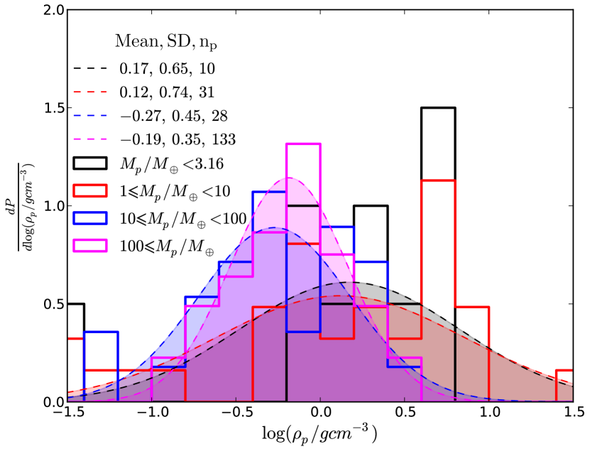
Figure 1.— Probability distribution functions for $\log(\rho_{p}/\rm{g\>cm^{-3}})$ of observed planets with known $M_{p}$ and $R_{p}$. Full set is divided into four groups contained in equal logarithmic bins of $M_{p}/{M_{\oplus}}$, $0.1$–$1$ (black), $1$–$10$ (red), $10$–$10^{2}$ (blue), $10^{2}$–$10^{3}$ (magenta). Since no exoplanets with known $M_{p}$ and $R_{p}$ populate the first group $0.1\leq(M_{p}/M_{\oplus})<1$, we estimate the $\rho_{p}$-distribution by taking into account all planets with $M_{p}/M_{\oplus}\leqslant 3.16$. Solid histograms and filled dashed lines show distributions of actual data and best-fit lognormals, respectively. Legend shows mean and standard deviation for each distribution, and number of planets in each group (left to right, respectively).

2. Innermost Planet Mass vs Orbital Radius Relation

IOPF theory predicts that position of formation of the innermost planet is determined by DZIB location, first set by thermal ionzation of alkali metals at disk midplane temperatures $T\simeq 1200\>\,{\rm K}$. Predicting this location is expected to be relatively simple compared to locations of subsequent planet formation, which depend on extent of DZIB retreat, which depends on reduction of disk gas column density caused by presence of the first planet. Ionization fraction may then increase further out in the disk either via increased midplane temperatures from higher protostellar heating or via increased received X-ray flux from the protostar or disk corona (e.g., Mohanty et al., 2013).

Following CT14, the predicted formation location of the innermost planet using the fiducial Shakura-Sunyaev steady viscous active accretion disk model, and assuming negligible protostellar heating, is

$$r_{1200{\rm K}}=0.178{\phi_{\rm{DZIB}}}\gamma_{1.4}^{-2/9}\kappa_{10}^{2/9}\alpha_{-3}^{-2/9}m_{*,1}^{1/3}(f_{r}\dot{m}_{-9})^{4/9}\>{\rm AU}.$$ (1)

Here $\gamma\equiv 1.4\gamma_{1.4}$ is the power-law exponent of the barotropic equation of state $P=K\rho^{\gamma}$ ($P$ and $\rho$ are midplane pressure and density), $\kappa\equiv 10\kappa_{10}\>{\rm cm^{2}\>g^{-1}}$ is disk opacity, $\alpha\equiv 10^{-3}\alpha_{-3}$ is viscosity parameter, $m_{\star}\equiv m_{\star,1}\>{M_{\odot}}$ is stellar mass, $\dot{m}\equiv 10^{-9}\dot{m}_{-9}\>{M_{\odot}\rm{yr}^{-1}}$ is accretion rate, and $f_{r}\equiv 1-\sqrt{r_{\star}/r}$ where $r_{\star}$ is stellar radius. Note that the choice of normalization for $\alpha$ reflects expected values in the dead-zone region near the DZIB, and this value is quite uncertain (CT14). Eq. 1 is the same as Eq. 11 of CT14 except, we have added an additional parameter ${\phi_{\rm{DZIB}}}$ to account for the fact that the estimate of midplane temperature can be affected by several factors, including energy extraction from a disk wind and protostellar heating. By comparison with more realistic protostellar disk models of Zhang et al. (2013), CT14 argued for a potential reduction in $r_{1200{\rm{K}}}$ by a factor of two, perhaps also due to reduction in $\kappa$ as dust grains begin to be destroyed. Thus for our fiducial model, here we will use ${\phi_{\rm{DZIB}}}=0.5$.

At the location given in Eq. 1, a forming planet may grow in mass, most likely by pebble accretion, to a gap opening mass determined by the viscous-thermal criterion (Lin & Papaloizou, 1993),

$$M_{p} = \frac{\phi_{G}40{\nu}m_{*}}{r^{2}\Omega_{K}}$$

$$= 20\frac{3^{1/5}}{\pi^{2/5}}\phi_{G}\left(\frac{\mu}{\gamma k_{B}}\right)^{-4/5}\left(\frac{\kappa}{\sigma_{\rm{SB}}}\right)^{1/5}$$

$$\times \alpha^{4/5}G^{-7/10}m_{*}^{3/10}\left(f_{r}\dot{m}\right)^{2/5}r^{1/10}$$

$$\rightarrow 5.67\phi_{G,0.3}\gamma_{1.4}^{4/5}\kappa_{10}^{1/5}\alpha_{-3}^{4/5}m_{*,1}^{3/10}(f_{r}\dot{m}_{-9})^{2/5}r_{\rm{AU}}^{1/10}\>M_{\oplus},$$

(Eq. 26 of CT14) where we adopt $\phi_{G}=0.3$ (Zhu et al., 2013) and $r$ is orbital radius of the forming planet. An uncertain quantity here is $\dot{m}$, which may vary widely from system to system and over time within a system.

We eliminate the accretion rate term, $f_{r}\dot{m}$, from Eq. 2 using Eq. 1 and set $r=r_{\rm 1200K}$ to find the innermost planet mass, $M_{p,1}$, (i.e., gap opening mass at DZIB) as a function of $r$:

$$M_{p,1}=5.0\phi_{G,0.3}{\phi_{\rm{DZIB}}}_{0.5}^{-9/10}\gamma_{1.4}\alpha_{-3}(r_{\rm{AU}}/0.1)\>{M_{\oplus}},$$ (3)

i.e., $M_{p,1}\propto r_{\rm{AU}}$: a linear increase in innermost planet mass with orbital radius of formation. Note, variation in $r$ is caused by variation in $\dot{m}$: higher $\dot{m}$ results in $T=1200$ K at larger radius. The dependence on $\kappa$ and $m_{*}$ vanish. The normalization of the $M_{p,1}$-$r$ relation depends on $\phi_{G}$, $\phi_{\rm DZIB}$, $\gamma$ and $\alpha$.

If subsequent planetary migration is negligible, then Equation 3’s prediction can be compared directly with the observed STIPs innermost planets. Two arguments suggest planetary migration from the initial formation site may be small. First, when the planet is still forming and has not yet opened a gap, drastic change in $\alpha$ at the DZIB creates an outwardly increasing surface density gradient and unsaturated corotation torques suppress Type I migration (Paardekooper & Papaloizou, 2009; Lyra et al., 2010) creating a “planet trap” at the (DZIB) pressure maximum (Masset et al., 2006; Matsumura et al., 2009). Second, when the planet is massive enough to open a gap, its mass already dominates over that in the inner gas disk, limiting scope for Type II migration.

3. Mass, radius, and density of KPCs

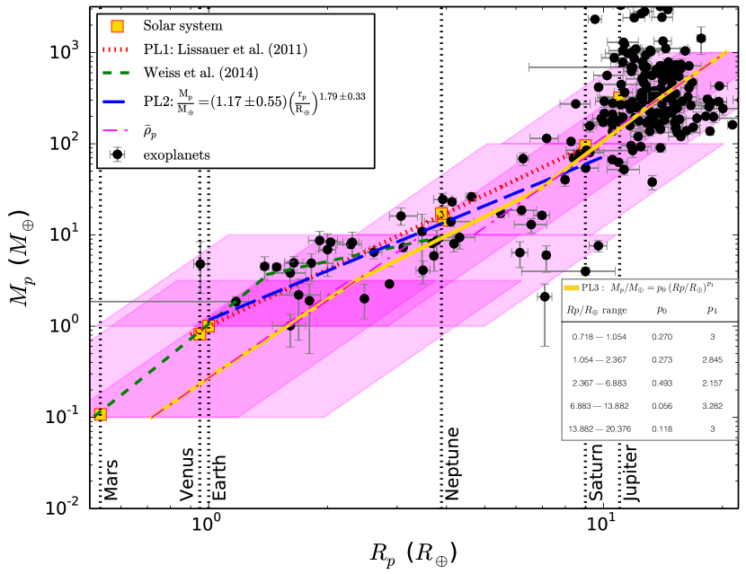
Figure 2.— $M_{p}$ versus $R_{p}$ for planets with direct measurements of mass and size. Vertical dotted lines and yellow squares show Solar System planets. Black dots denote exoplanets. Dotted (red), dashed (green), long-dashed (blue), and solid (gold) lines show simple power-law $M_{p}$-$R_{p}$ relations proposed by Lissauer et al. (2011), Weiss & Marcy (2014), our own best fit power-law $M_{p}/{M_{\oplus}}=(1.17\pm 0.55)(R_{p}/{R_{\oplus}})^{(1.79\pm 0.33)}$ over similar range as Lissauer et al. (2011), and piecewise estimated power-laws based on fitted mean planetary densities in equal intervals of log $M_{p}$ (Fig. 1), respectively. Dash-dot line traces the mean $\rho_{p}$. Darker and fainter shaded regions denote $1$ and $2\sigma$ of best-fit lognormal PDFs as a function of $M_{p}$ (Fig. 1).

While IOPF (CT14) predicts $M_{p}$, planets of the same mass may attain widely varying average densities ($\rho_{p}$) depending on relative importance of gas and pebble accretion and also atmospheric puffiness, dependent on detailed atmospheric properties (e.g., Howe et al., 2014). Thus predicting $R_{p}$ is not straightforward within the framework of IOPF. However, only $R_{p}$ is measured for most Kepler-discovered systems, and especially the smaller planets exhibit wide ranges of $\rho_{p}$ even when they are of comparable sizes (e.g., Howe et al., 2014; Gautier et al., 2012; Masuda, 2014). Also, both mean and overall range of $\rho_{p}$ vary based on the planet mass range under consideration (e.g., Weiss & Marcy, 2014; Howe et al., 2014, Fig. 1). Hence, direct comparison between theory and observation is difficult for individual planets and a statistical approach is needed.

To convert IOPF-predicted $M_{p}$ into a corresponding $R_{p}$, probability distribution functions (PDFs) for $\rho_{p}$ that change continuously as a function of $M_{p}$ would be ideal. Radial velocity (RV) follow-up and transit timing variation (TTV) measurements have constrained $M_{p}$ for some Kepler systems (Marcy et al., 2014, for a list). However, the small number of observed planets where $\rho_{p}$ could be measured limits how finely the different $M_{p}$ ranges can be sampled. For this study, we divide the set of planets with known $\rho_{p}$ crudely in four groups, each ranging over 1 dex in $M_{p}$ with boundaries at $0.1,1,10,10^{2}$, and $10^{3}\>{M_{\oplus}}$. Since no exoplanets with measured $\rho_{p}$ have $(M_{p}/M_{\oplus})<1$, we include planets with $M_{p}$ up to half a dex into the next group to determine the $\rho_{p}$-distribution for mass group $0.1\leq(M_{p}/{M_{\oplus}})<1$. We estimate the observed $\rho_{p}$ PDFs for each group separately by fitting lognormals (Fig. 1). We assume that all planets within each mass group have the same PDF for $\rho_{p}$. We use the appropriate $\rho_{p}$-distribution for an IOPF-predicted $M_{p}$ for a given $r$, to randomly generate the average density and calculate $R_{p}$ in §4. Note that this division in groups is quite arbitrary, but necessary given the available data.

$M_{p}$ values of the thousands of KPCs with measured $R_{p}$ are often estimated using simple power-law relations, derived based on planets with measured $M_{p}$ from RV followup and TTV (Marcy et al., 2014). Although, choosing a simple $M_{p}$-$R_{p}$ power-law relation essentially ignores $\rho_{p}$ dispersions at a fixed $R_{p}$, they are popular because of their simplicity. Fig. 2 shows a compilation of the data for planets with directly measured $M_{p}$ and $R_{p}$, together with two previously published fitted $M_{p}$-$R_{p}$ power-law relations by Lissauer et al. (2011, henceforth PL1) and Weiss & Marcy (2014). We also include our own best fit power-law relation following Lissauer et al. (2011) for planets between $1\leq(R_{p}/{R_{\oplus}})\leq 10$, but not forcing the relation to match the Earth. We derive $(M_{p}/{M_{\oplus}})=(1.17\pm 0.55)(R_{p}/{R_{\oplus}})^{(1.79\pm 0.33)}$ (henceforth PL2) by fitting data with uniform weighting, independent of measurement errors. This choice is made since we expect the spread in masses at a given radius reflects an intrinsic dispersion in density and we wish to avoid the average relation of the planet population being biased towards the systems that happen to have the smallest errors. Finally, we construct a piecewise power-law (henceforth PL3) by connecting the $R_{p}$ and $M_{p}$ values at the middle $R_{p}$ points in each $M_{p}$ group and the mean of $\log\>R_{p}$ values at the group boundaries along the mean $\log\rho_{p}$ lines in each group; $M_{p}/{M_{\oplus}}=p_{0}(R_{p}/{R_{\oplus}})^{p_{1}}$, $R_{p}/{R_{\oplus}}$ intervals $=\left\{0.718,1.054,2.367,6.883,13.882,20.376\right\}$, $p_{0}=\left\{0.270,0.273,0.493,0.056,0.118\right\}$, $p_{1}=\left\{3,2.845,2.157,3.282,3\right\}$.

The estimated $M_{p}$ can thus be different for the same observed $R_{p}$ depending on which power-law is used. However, Fig. 2 shows that the intrinsic dispersion in $M_{p}$ at a given $R_{p}$, due to a dispersion in $\rho_{p}$, is larger than the differences between the power laws. For completeness we will use all three power-laws PL1–3 to estimate $M_{p}$ for a given $R_{p}$ and show the resulting differences. For this study we do not use the power-law proposed by Weiss & Marcy (2014) since its applicability is within a limited range in $R_{p}\leq 4\,{R_{\oplus}}$.

4. Comparison with observed Kepler systems

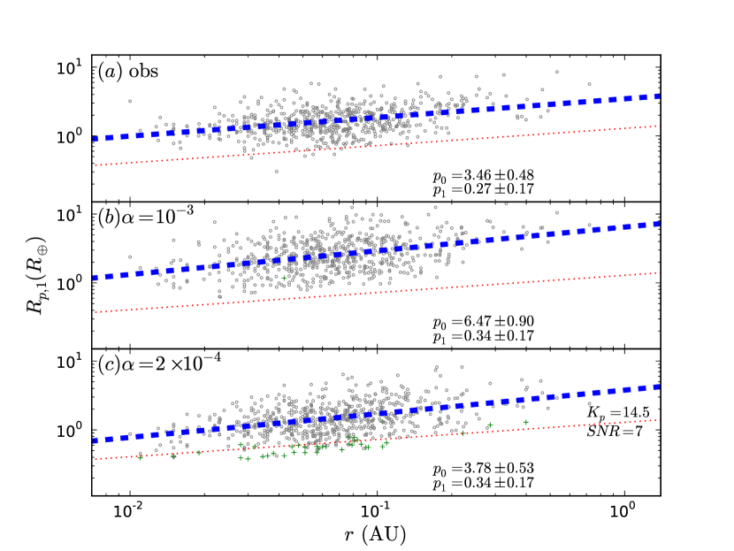
Figure 3.— Planetary radius of innermost planets ($R_{p,1}$) in multiplanet systems as a function of $r$ (grey dots). Green ’+’s denote planets discarded because they would not be detectable by Kepler. Blue dashed line represents best-fit power-law $R_{p,1}/{R_{\oplus}}=p_{0}r_{\rm{AU}}^{p_{1}}$. Red dotted lines show detection limit (SNR=7) for median $K_{p}=14.5$ of host stars in the observed sample. (a) Top: Observed Kepler population. (b) Middle: Synthetically generated planet population from IOPF (§4) using $\alpha=10^{-3}$. (c) Bottom: As (b), but for $\alpha=2\times 10^{-4}$. Best-fit values of $p_{0}$ and $p_{1}$ are shown in each panel, including $1\sigma$ errors. Within statistical fluctuations, $p_{1}$ values for the synthetic populations (both $\alpha$s) agree well with the observed scaling.

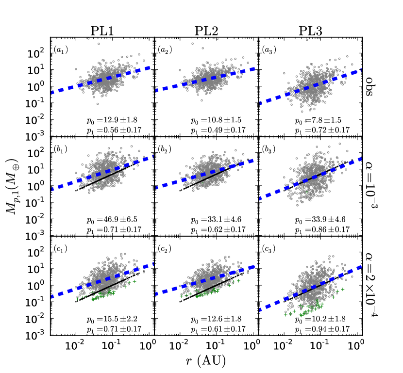
Figure 4.— Mass of innermost planets ($M_{p,1}$) in multiplanet systems versus $r$. Left to right, panels show $M_{p,1}$ values obtained using PL1–3, respectively (§3). Top to bottom, panels show observed and synthetic data with $\alpha=10^{-3}$ and $2\times 10^{-4}$, respectively (§4). Black dots denote the actual $M_{p,1}$ of the synthetic data, following Eq. 3. Grey dots denote estimated $M_{p,1}$ for a given $R_{p}$ using one of the $M_{p}$-$R_{p}$ power-laws (PL1–3). Green ’+’s are undetectable planets. Blue dashed lines show best-fit power-laws $M_{p,1}/{M_{\oplus}}=p_{0}r_{\rm{AU}}^{p_{1}}$, $p_{0}$ and $p_{1}$ with $1\sigma$ errors shown in each panel. PL1,2 systematically predict a higher $\rho_{p}$ for a given $R_{p}$ relative to our fitted lognormal mean $\rho_{p}$ (Fig. 2) resulting in typically higher estimated masses compared to actual $M_{p}$.

Since we are interested in testing whether properties of STIPs innermost planets are consistent with IOPF predictions, we restrict ourselves only to innermost KPCs in multiplanet systems ($n_{p}\geq 2$). We obtain KPC data from NASA’s exoplanet archive (http://exoplanetarchive.ipac.caltech.edu; June 25, 2014 update). We find that for the 629 multi-transiting systems, $R_{p,1}/{R_{\oplus}}=(3.5\pm 0.5)r_{\rm{AU}}^{(0.3\pm 0.2)}$, where errors are $1\sigma$ obtained from parameter estimation and fitting is done using equal weight to each data point (Fig. 3a).

While creating the synthetic innermost planet populations based on the IOPF model we pay attention to replicate all observational biases in the observed sample as closely as possible. We import the period $P$, semimajor axis $a$, assumed to be equal to $r$ (low eccentricity), $r_{\star}$, and Kepler magnitude ($K_{p}$) for the innermost KPCs. This way our synthetic planet sample automatically preserves the observed distribution of planetary orbital and host star properties. For a given $r$ we use Eq. 3 to determine $M_{p}$ as predicted by IOPF. Densities are then randomly assigned by drawing from the appropriate lognormal PDFs (§3). We restrict $\rho_{p}$ to be between $32$ and $0.01\>\rm{g\>cm^{-3}}$ (Howe et al., 2014; Masuda, 2014). Our conclusions are not very sensitive to reasonable changes in the $\rho_{p}$ range. Note, the actual total range in $\rho_{p}$ is unknown and transit observations are biased towards detecting lower density planets in general. Planet size $R_{p}$ is calculated using $M_{p}$ and $\rho_{p}$. Using host star $K_{p}$ values we estimate the combined differential photometric precision following Gilliland et al. (2011, see for details). We then estimate whether this synthetic planet would be detectable (SNR$>7$ assuming $3.5\,{\rm yr}$ observation) by Kepler. We repeat this process until we generate one Kepler-detectable planet for each host star. Examples of synthetic populations, each of $629$ detectable planets, are shown in Fig. 3(b) using $\alpha=10^{-3}$, and (c) using $\alpha=2\times 10^{-4}$.

We find IOPF-predicted $R_{p,1}$ versus $r$, $R_{p,1}/{R_{\oplus}}\propto r_{\rm{AU}}^{0.3\pm 0.2}$, shows very similar scaling as that of the observed planets. The absolute normalization is somewhat arbitrary and depends on unconstrained disk properties including $\alpha$ and ${\phi_{\rm{DZIB}}}$. For example, while the scaling remains very similar, the proportionality constant changes with a change of the adopted value of $\alpha$. For $\alpha=2\times 10^{-4}$ both the scaling and the normalization agree well for the $R_{p,1}$–$r$ relations in the observed and synthetic samples.

Turning to masses, the $M_{p,1}$-$r$ relation depends on the adopted $M_{p}$-$R_{p}$ relation. For PL1–3 these are given as $M_{p,1}=(12.9\pm 1.8)r_{\rm{AU}}^{(0.56\pm 0.17)},\>(10.8\pm 1.5)r_{\rm{AU}}^{(0.49\pm 0.17)},\>(7.8\pm 1.5)=r_{\rm{AU}}^{(0.72\pm 0.17)}$, respectively for the observed sample (Fig. 4). Thus, adopting a simple $M_{p}$-$R_{p}$ relation, or equivalently, assuming a fixed $\rho_{p}$ for a given $R_{p}$ in estimating $M_{p}$ results in $M_{p,1}$-$r$ scalings that are shallower than the linear prediction of IOPF (Eq. 3).

Fig. 4 shows the comparison between observed and synthetic populations for PL1–3 and for $\alpha=10^{-3}$ and $2\times 10^{-4}$. We find that for all considered simple $M_{p}$-$R_{p}$ relations (PL1–3), best-fit power laws for observed and predicted planet populations agree reasonably well. As for the $R_{p,1}$-$r$ relations, the scalings agree within expected statistical fluctuations for both $\alpha$ values. The normalization is again off by a factor of a few for $\alpha=10^{-3}$, but is quite similar for $\alpha=2\times 10^{-4}$ for all $M_{p}$-$R_{p}$ power-laws. It is also instructive to see the degree to which estimated $M_{p}$ can diverge from actual $M_{p}$ due to the assumption of fixed $\rho_{p}$ for fixed $R_{p}$, or equivalently, assuming a simple power-law relation between $R_{p}$ and $M_{p}$. Using such power-laws, while useful for a crude estimate of $M_{p}$ from an observed $R_{p}$, can lead to derived $M_{p}$ being very different from the actual one, due to the intrinsic dispersion in density. This highlights the importance of further TTV analysis and RV followup.

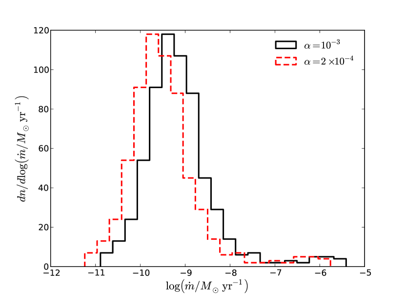
Figure 5.— Histogram of effective mass accretion rate ($\dot{m}$) for creation of the innermost observed planets in Kepler’s multitransiting systems. The $\dot{m}$ values are calculated using fiducial values described in §2 and $\alpha=10^{-3}$ (black solid) and $2\times 10^{-4}$ (red dashed). The innermost planet candidates are chosen as described in §4. For $\alpha=2\times 10^{-4}$ the $16$, $50$, and $84$th percentiles are $7.2\times 10^{-11}$, $2.6\times 10^{-10}$, and $1.2\times 10^{-9}\>{M_{\odot}\>\rm yr^{-1}}$, respectively.

Assuming that our selected observed sample of innermost planets truly are innermost, “Vulcan” planets, their observed orbital radii can also constrain $\dot{m}$ via Eq. 1. Figure 5 shows histograms of the expected $\dot{m}$ for the observed systems if formed via IOPF. The estimated effective $\dot{m}$ for a given innermost planet’s position depends on $\alpha$. We find that the majority of the observed sample of innermost planets predict effective $\dot{m}$ between $\sim 10^{-11}$–$10^{-8}\>{M_{\odot}\rm{yr}^{-1}}$ for $\alpha=2\times 10^{-4}$. The tail towards very large $\dot{m}\gtrsim 10^{-7}$ may indicate that some selected planets are not actually innermost planets: either there is an undetected inner planet (Nesvorný et al., 2012, 2013; Barros et al., 2014), or perhaps the original inner planet has been removed via, for example, collision or ejection.

5. Discussion and Conclusions

We showed that IOPF predicts STIPs innermost planet mass, $M_{p,1}$, increases linearly with $r$, independent of $\dot{m}$, $m_{*}$, or $\kappa$. Absolute values for $M_{p,1}$, however, depend strongly on disk properties, especially viscosity parameter $\alpha$.

Using fiducial disk parameters and observationally motivated mass-based density ranges we found the IOPF $R_{p,1}$-$r$ scaling is consistent with that in observed Kepler multis (Fig. 3). Comparing mass scalings involved assuming a $M_{p}$-$R_{p}$ relation (Fig. 2). The estimated $M_{p,1}$-$r$ scalings vary depending on which $M_{p}$-$R_{p}$ relation was chosen, even when the real underlying relation is $M_{p,1}\propto{r}$. We showed that $M_{p,1}$-$r$ scalings for theoretical and observed populations agree within expected uncertainties for all adopted $M_{p}$-$R_{p}$ relations. Assuming formation via IOPF, the distribution of $r$ for the innermost planets implies $\dot{m}$ between $\sim 10^{-10}$–$10^{-9}\>{M_{\odot}\rm{yr}^{-1}}$, adopting our preferred DZIB $\alpha=2\times 10^{-4}$.

For comparison between the IOPF predicted and observed inner planet properties we had to make several simplifying assumptions. We assumed the $M_{p}$-based $\rho_{p}$ distributions for STIPs innermost planets are similar to those obtained from all planets with known $\rho_{p}$. However, IOPF innermost planets, forming very close to the star, potentially have quite different entropy structure in their atmospheres and thus systematically different densities compared to planets that form further out. We have also assumed that the apparent innermost planet in multitransiting systems are truly so. Limiting the observed sample to only multitransiting systems and only out to $r=1\>{\rm{AU}}$ alleviates this problem somewhat.

The exact $R_{p,1}$-$r$ and $M_{p,1}$-$r$ relations for the synthetic planet population predicted by IOPF depend somewhat on the $M_{p}$-based $\rho_{p}$ distributions adopted. However, for several observationally motivated $\rho_{p}$ distributions we find agreement between the theoretical and observed populations. Nevertheless, since the $\rho_{p}$ PDF in the lowest-mass bin is the most important in determining the fraction of detectable small planets in a synthetic population, more observational constraints on densities of low-mass planets ($M_{p}<1{M_{\oplus}}$) will be very useful for a more robust comparison. Continued efforts for RV followup and TTV measurements will potentially lead to more mass measurements making a more direct comparison possible for testing IOPF theory. Another source of change in the final $M_{p,1}$ and $R_{p,1}$ vs $r$ relations is possible inward migration of some planets after they have formed via IOPF, which needs to be investigated in future numerical simulations.

Finally, we point out that there may be other mechanisms that can help create $M_{p}$ vs $r$ correlations. For example, increasing planet mass with radius may be related to radial dependence of massloss via stellar irradiation (Lopez et al., 2012). A quantitative calculation of the effects of this mass-loss, which will tend to steepen the IOPF $M_{p,1}$ vs $r$ relation, will require modeling the composition and size of the planets, as well as the history of their EUV and X-ray flux exposure.

References

- Barros et al. (2014) Barros, S. C. C., Díaz, R. F., Santerne, A., Bruno, G., et al. 2014, A&A, 561, L1
- Baruteau & Papaloizou (2013) Baruteau, C. & Papaloizou, J. C. B. 2013, ApJ, 778, 7
- Batygin & Morbidelli (2013) Batygin, K. & Morbidelli, A. 2013, AJ, 145, 1
- Chatterjee & Ford (2014) Chatterjee, S. & Ford, E. B. 2014, arXiv:1406.0512
- Chatterjee et al. (2012) Chatterjee, S., Ford, E. B., Geller, A. M., & Rasio, F. A. 2012, MNRAS, 427, 1587
- Chatterjee et al. (2008) Chatterjee, S., Ford, E. B., Matsumura, S., & Rasio, F. A. 2008, ApJ, 686, 580
- Chatterjee & Tan (2014) Chatterjee, S. & Tan, J. C. 2014, ApJ, 780, 53
- Chiang & Laughlin (2013) Chiang, E. & Laughlin, G. 2013, MNRAS, 431, 3444
- Cossou et al. (2014) Cossou, C., Raymond, S. N., Hersant, F., & Pierens, A. 2014, arXiv:1407.6011
- Cossou et al. (2013) Cossou, C., Raymond, S. N., & Pierens, A. 2013, A&A, 553, L2
- Fang & Margot (2012) Fang, J. & Margot, J.-L. 2012, ApJ, 761, 92
- Gautier et al. (2012) Gautier, III, T. N., Charbonneau, D., Rowe, J. F., Marcy, G. W., et al. 2012, ApJ, 749, 15
- Gilliland et al. (2011) Gilliland, R. L., Chaplin, W. J., Dunham, E. W., Argabright, V. S., et al. 2011, ApJS, 197, 6
- Goldreich & Schlichting (2014) Goldreich, P. & Schlichting, H. E. 2014, AJ, 147, 32
- Hansen & Murray (2012) Hansen, B. M. S. & Murray, N. 2012, ApJ, 751, 158
- Hansen & Murray (2013) —. 2013, ApJ, 775, 53
- Howe et al. (2014) Howe, A. R., Burrows, A., & Verne, W. 2014, ApJ, 787, 173
- Hu et al. (2014) Hu, X., Tan, J. C., & Chatterjee, S. 2014, arXiv:1410.5819
- Kley & Nelson (2012) Kley, W. & Nelson, R. P. 2012, ARA&A, 50, 211
- Lin & Papaloizou (1993) Lin, D. N. C. & Papaloizou, J. C. B. 1993, in Protostars and Planets III, ed. E. H. Levy & J. I. Lunine, 749–835
- Lissauer et al. (2011) Lissauer, J. J., Ragozzine, D., Fabrycky, D. C., Steffen, J. H., et al. 2011, ApJS, 197, 8
- Lithwick & Wu (2012) Lithwick, Y. & Wu, Y. 2012, ApJ, 756, L11
- Lopez et al. (2012) Lopez, E. D., Fortney, J. J., & Miller, N. 2012, ApJ, 761, 59
- Lyra et al. (2010) Lyra, W., Paardekooper, S.-J., & Mac Low, M.-M. 2010, ApJ, 715, L68
- Marcy et al. (2014) Marcy, G. W., Isaacson, H., Howard, A. W., Rowe, J. F., et al. 2014, ApJS, 210, 20
- Masset et al. (2006) Masset, F. S., Morbidelli, A., Crida, A., & Ferreira, J. 2006, ApJ, 642, 478
- Masuda (2014) Masuda, K. 2014, ApJ, 783, 53
- Matsumoto et al. (2012) Matsumoto, Y., Nagasawa, M., & Ida, S. 2012, Icarus, 221, 624
- Matsumura et al. (2009) Matsumura, S., Pudritz, R. E., & Thommes, E. W. 2009, ApJ, 691, 1764
- Mohanty et al. (2013) Mohanty, S., Ercolano, B., & Turner, N. J. 2013, ApJ, 764, 65
- Nagasawa & Ida (2011) Nagasawa, M. & Ida, S. 2011, ApJ, 742, 72
- Nesvorný et al. (2013) Nesvorný, D., Kipping, D., Terrell, D., Hartman, J., Bakos, G. Á., & Buchhave, L. A. 2013, ApJ, 777, 3
- Nesvorný et al. (2012) Nesvorný, D., Kipping, D. M., Buchhave, L. A., Bakos, G. Á., Hartman, J., & Schmitt, A. R. 2012, Science, 336, 1133
- Paardekooper & Papaloizou (2009) Paardekooper, S.-J. & Papaloizou, J. C. B. 2009, MNRAS, 394, 2283
- Papaloizou (2011) Papaloizou, J. C. B. 2011, Celestial Mechanics and Dynamical Astronomy, 111, 83
- Petrovich et al. (2013) Petrovich, C., Malhotra, R., & Tremaine, S. 2013, ApJ, 770, 24
- Rasio & Ford (1996) Rasio, F. A. & Ford, E. B. 1996, Science, 274, 954
- Raymond & Cossou (2014) Raymond, S. N. & Cossou, C. 2014, MNRAS, 440, L11
- Rein (2012) Rein, H. 2012, MNRAS, 427, L21
- Schlichting (2014) Schlichting, H. E. 2014, ApJ, 795, L15
- Weiss & Marcy (2014) Weiss, L. M. & Marcy, G. W. 2014, ApJ, 783, L6
- Zhang et al. (2013) Zhang, Y., Tan, J. C., & McKee, C. F. 2013, ApJ, 766, 86
- Zhu et al. (2013) Zhu, Z., Stone, J. M., & Rafikov, R. R. 2013, ApJ, 768, 143