Exact solution of a generalized version
of the Black-Scholes equation

Abstract

We analyze a generalized version of the Black-Scholes equation depending on a parameter $a\!\in\!(-\infty,0)$. It satisfies the martingale condition and coincides with the Black-Scholes equation in the limit case $a\nearrow 0$. We show that the generalized equation is exactly solvable in terms of Hermite polynomials and numerically compare its solution with the solution of the Black-Scholes equation.

1 Introduction

The mathematical model based on the Black-Scholes equation

$$\frac{\partial C}{\partial t}=-\frac{\sigma^{2}}{2}S^{2}\frac{\partial^{2}C}{\partial S^{2}}-rS\frac{\partial C}{\partial S}+rC$$ (1)

anticipates rather well the observed prices for options in the case of a strike price that is not too far from the current price of the underlying asset [8]. The price of an option at a moment of time $t$ depends on the current price $S$, the volatility $\sigma$, the risk-free interest rate $r$, the strike price $K$ and the maturity time $T$. In the case of an European option, the price is described by the solution $C(S,t)$ of equation (1) satisfying the condition

$$C(S,T)=\left\{\begin{array}[]{cll}S\!-\!K&\mbox{if}&S\!\geq\!K\\[5.69054pt] 0&\mbox{if}&S\!<\!K\end{array}\right.$$ (2)

in the case of a call option, and

$$C(S,T)=\left\{\begin{array}[]{cll}0&\mbox{if}&S\!\geq\!K\\[5.69054pt] K\!-\!S&\mbox{if}&S\!<\!K\end{array}\right.$$ (3)

in the case of a put option. The alternative version of the equation (1)

$$\frac{\partial\tilde{C}}{\partial t}=-\frac{\sigma^{2}}{2}\frac{\partial^{2}\tilde{C}}{\partial x^{2}}+\left(\frac{\sigma^{2}}{2}-r\right)\frac{\partial\tilde{C}}{\partial x}+r\tilde{C}$$ (4)

obtained by using the change of independent variable

$$S={\rm e}^{x}$$ (5)

allows one to use the formalism of quantum mechanics in option pricing [1, 2, 4, 7]. In the new variable the conditions (2) and (3) become

$$\tilde{C}(x,T)=\left\{\begin{array}[]{cll}{\rm e}^{x}\!-\!K&\mbox{if}&x\!\geq\!\ln K\\[5.69054pt] 0&\mbox{if}&x\!<\!\ln K\end{array}\right.$$ (6)

and respectively,

$$\tilde{C}(x,T)=\left\{\begin{array}[]{cll}0&\mbox{if}&x\!\geq\!\ln K\\[5.69054pt] K\!-\!{\rm e}^{x}&\mbox{if}&x\!<\!\ln K\,.\end{array}\right.$$ (7)

The more general version of (4) depending on a function $V(x)$

$$\frac{\partial\tilde{C}}{\partial t}=-\frac{\sigma^{2}}{2}\frac{\partial^{2}\tilde{C}}{\partial x^{2}}+\left(\frac{\sigma^{2}}{2}-V(x)\right)\frac{\partial\tilde{C}}{\partial x}+V(x)\,\tilde{C}$$ (8)

satisfies the martingale condition [1] and hence can be used for studying processes in finance. Our purpose is to investigate the particular case

$$V(x)=ax+r$$ (9)

that is, the equation

$$\frac{\partial\tilde{C}}{\partial t}=-\frac{\sigma^{2}}{2}\frac{\partial^{2}\tilde{C}}{\partial x^{2}}+\left(\frac{\sigma^{2}}{2}-ax\!-\!r\right)\frac{\partial\tilde{C}}{\partial x}+(ax\!+\!r)\tilde{C}$$ (10)

where $a\!\in\!(-\infty,0)$ is a parameter. The equation (10) is exactly solvable in terms of Hermite polynomials and coincides in the limit case $a\nearrow 0$ with the equation (4) which corresponds to the standard Black-Scholes equation.

2 A shifted oscillator

Let $\alpha\!\in\!(-\infty,0)$ and $\beta\!\in\!\mathbb{R}$ be two constants. By using the Hermite polynomial

$${\bf H}_{n}(s)=(-1)^{n}\ {\rm e}^{s^{2}}\ \frac{d^{n}}{ds^{n}}({\rm e}^{-s^{2}})$$ (11)

we define for each $n\!\in\!\{0,1,2,...\}$ the function

$$\begin{array}[]{l}\psi_{n}(x)=\frac{1}{\sqrt{n!\,2^{n}}}\sqrt[4]{\frac{-\alpha}{2\pi}}\ {\rm e}^{\frac{\alpha}{4}x^{2}+\frac{\beta}{2}x+\frac{\beta^{2}}{4\alpha}}\ {\bf H}_{n}\left(\sqrt{\frac{-\alpha}{2}}x-\frac{\beta}{\sqrt{-2\alpha}}\right).\end{array}$$ (12)

If we denote

$$\begin{array}[]{l}s=\sqrt{\frac{-\alpha}{2}}x-\frac{\beta}{\sqrt{-2\alpha}}\end{array}$$ (13)

then the previous relation can be written as

$$\begin{array}[]{l}{\bf H}_{n}(s)=\sqrt{n!\,2^{n}}\,\sqrt[4]{\frac{2\pi}{-\alpha}}\ {\rm e}^{\frac{1}{2}s^{2}}\ \psi_{n}\left(\sqrt{\frac{2}{-\alpha}}s-\frac{\beta}{\alpha}\right).\end{array}$$ (14)

By substituting this relation into the diferential equation

$${\bf H}^{\prime\prime}_{n}(s)-2s{\bf H}_{n}^{\prime}(s)+2n{\bf H}_{n}(s)=0$$ (15)

satisfied by the Hermite polynomial ${\bf H}_{n}$ we get the equality

$$\begin{array}[]{l}-\psi_{n}^{\prime\prime}\left(\sqrt{\frac{2}{-\alpha}}s-\frac{\beta}{\alpha}\right)+\left(-\frac{\alpha}{2}s^{2}+\frac{\alpha}{2}+\alpha n\right)\ \psi_{n}\left(\sqrt{\frac{2}{-\alpha}}s-\frac{\beta}{\alpha}\right)=0\end{array}$$ (16)

which can be written in the form

$$\left(-\frac{\partial^{2}}{\partial x^{2}}+\frac{(\alpha x\!+\!\beta)^{2}}{4}+\frac{\alpha}{2}\right)\psi_{n}=-\alpha n\,\psi_{n}.$$ (17)

This means that $\psi_{n}$ is an eigenfunction of the shifted oscillator [3, 5, 6].

$$H=-\frac{\partial^{2}}{\partial x^{2}}+\frac{(\alpha x\!+\!\beta)^{2}}{4}+\frac{\alpha}{2}$$ (18)

corresponding to the eigenvalue $\lambda_{n}\!=\!-\alpha n$, for any $n\!\in\!\{0,1,2,...\}$. Since

$$\int_{-\infty}^{\infty}{\rm e}^{-s^{2}}\ {\bf H}_{n}(s)\ {\bf H}_{k}(s)\ ds=\left\{\begin{array}[]{cll}n!\,2^{n}\sqrt{\pi}&{\rm if}&n\!=\!k\\[5.69054pt] 0&{\rm if}&n\!\neq\!k\end{array}\right.$$ (19)

the system of functions $\{\psi_{n}\}_{n=0,1,2,...}$ is orthonormal, that is,

$$\int_{-\infty}^{\infty}\psi_{n}(x)\ \psi_{k}(x)\ dx=\left\{\begin{array}[]{cll}1&{\rm if}&n\!=\!k\\[5.69054pt] 0&{\rm if}&n\!\neq\!k.\end{array}\right.$$ (20)

One can prove that it is complete in the space of square integrable functions.

3 A generalized version of the Black-Scholes equation

A straightforward generalization of the equation

$$\frac{\partial\tilde{C}}{\partial t}=-\frac{\sigma^{2}}{2}S^{2}\frac{\partial^{2}\tilde{C}}{\partial S^{2}}-rS\frac{\partial\tilde{C}}{\partial S}+r\tilde{C}$$ (21)

is the equation

$$\frac{\partial\tilde{C}}{\partial t}=-\frac{\sigma^{2}}{2}\frac{\partial^{2}\tilde{C}}{\partial x^{2}}+\left(\frac{\sigma^{2}}{2}-V(x)\right)\frac{\partial\tilde{C}}{\partial x}+V(x)\,\tilde{C}$$ (22)

satisfying the martingale condition [1]. It can be written in the form

$$\frac{\partial\tilde{C}}{\partial t}=H_{V}\tilde{C}$$ (23)

by using the Hamiltonian

$$H_{V}=-\frac{\sigma^{2}}{2}\frac{\partial^{2}}{\partial x^{2}}+\left(\frac{\sigma^{2}}{2}-V(x)\right)\frac{\partial}{\partial x}+V(x).$$ (24)

The Hamiltonian $H_{V}$ is equivalent with the Hermitian Hamiltonian

$$H_{\rm eff}=-\frac{\sigma^{2}}{2}\frac{\partial^{2}}{\partial x^{2}}+\frac{1}{2}\frac{\partial V}{\partial x}+\frac{1}{2\sigma^{2}}V^{2}+\frac{1}{2}V+\frac{\sigma^{2}}{8}$$ (25)

by the similarity transformation

$$H_{\rm eff}={\rm e}^{-u}H_{V}{\rm e}^{u}$$ (26)

where

$$u=\frac{1}{2}x-\frac{1}{\sigma^{2}}\int_{0}^{x}V(y)\,dy.$$ (27)

In the particular case $V(x)\!=\!ax\!+\!r$ considered in this article

$$\begin{array}[]{l}H_{V}=-\frac{\sigma^{2}}{2}\frac{\partial^{2}}{\partial x^{2}}+\left(\frac{\sigma^{2}}{2}-ax-r\right)\frac{\partial}{\partial x}+ax+r\\[11.38109pt] H_{\rm eff}=\frac{\sigma^{2}}{2}\left[-\frac{\partial^{2}}{\partial x^{2}}+\frac{1}{4}\left(\frac{2a}{\sigma^{2}}x+\frac{2r}{\sigma^{2}}+1\right)^{2}+\frac{a}{\sigma^{2}}\right]\\[11.38109pt] u=-\frac{a}{2\sigma^{2}}x^{2}-\left(\frac{r}{\sigma^{2}}-\frac{1}{2}\right)x.\end{array}$$ (28)

The Hamiltonian $H_{\rm eff}$ is up to the multiplicative factor $\frac{\sigma^{2}}{2}$ the Hamiltonian of a shifted oscillator, namely

$$H_{\rm eff}=\frac{\sigma^{2}}{2}H$$ (29)

where

$$\begin{array}[]{l}H=-\frac{\partial^{2}}{\partial x^{2}}+\frac{(\alpha x\!+\!\beta)^{2}}{4}+\frac{\alpha}{2}\end{array}$$ (30)

with

$$\begin{array}[]{l}\alpha=\frac{2a}{\sigma^{2}}\qquad\mbox{and}\qquad\beta=\frac{2r}{\sigma^{2}}\!+\!1.\end{array}$$

Therefore, for each $n\in\{0,1,2,...\}$ the function

$$\begin{array}[]{l}\psi_{n}(x)\!=\!\frac{1}{\sqrt{n!\,2^{n}\sigma}}\sqrt[4]{\frac{-a}{\pi}}\ {\rm e}^{\frac{a}{2\sigma^{2}}x^{2}+\left(\frac{r}{\sigma^{2}}+\frac{1}{2}\right)x+\frac{\sigma^{2}}{8a}\left(\frac{2r}{\sigma^{2}}+1\right)^{2}}{\bf H}_{n}\left(\frac{\sqrt{-a}}{\sigma}x-\frac{\sigma}{2\sqrt{-a}}\left(\frac{2r}{\sigma^{2}}\!+\!1\right)\right)\end{array}$$ (31)

is an eigenfunction of $H_{\rm eff}$ corresponding to the eigenvalue $-an$

$$\begin{array}[]{l}H_{\rm eff}\,\psi_{n}=-an\,\psi_{n}.\end{array}$$ (32)

The equation (23) can be written as

$$\frac{\partial\tilde{C}}{\partial t}={\rm e}^{u}H_{\rm eff}{\rm e}^{-u}\,\tilde{C}$$ (33)

or in the form

$$\frac{\partial}{\partial t}\,{\rm e}^{-u}\tilde{C}=H_{\rm eff}\,{\rm e}^{-u}\tilde{C}.$$ (34)

A function $\tilde{C}(x,t)$ is the solution of (23) satisfying (6) if and only if

$$\psi(x,t)={\rm e}^{-u}\tilde{C}(x,t)$$ (35)

that is, the function

$$\psi(x,t)={\rm e}^{\frac{a}{2\sigma^{2}}x^{2}+\left(\frac{r}{\sigma^{2}}-\frac{1}{2}\right)x}\tilde{C}(x,t)$$ (36)

is the solution of the equation

$$\frac{\partial\psi}{\partial t}=H_{\rm eff}\,\psi$$ (37)

satisfying the condition

$$\psi(x,T)={\rm e}^{\frac{a}{2\sigma^{2}}x^{2}+\left(\frac{r}{\sigma^{2}}-\frac{1}{2}\right)x}\left\{\begin{array}[]{cll}{\rm e}^{x}\!-\!K&\mbox{if}&x\!\geq\!\ln K\\[5.69054pt] 0&\mbox{if}&x\!<\!\ln K\,.\end{array}\right.$$ (38)

But, the solution of (37) satisfying (38) is

$$\psi(x,t)=\sum_{n=0}^{\infty}c_{n}\,{\rm e}^{-ant}\ \psi_{n}(x)$$ (39)

with the coefficients $c_{n}$ determined from the relation

$$\sum_{n=0}^{\infty}c_{n}\,{\rm e}^{-anT}\ \psi_{n}(x)={\rm e}^{\frac{a}{2\sigma^{2}}x^{2}+\left(\frac{r}{\sigma^{2}}-\frac{1}{2}\right)x}\left\{\begin{array}[]{cll}{\rm e}^{x}\!-\!K&\mbox{if}&x\!\geq\!\ln K\\[5.69054pt] 0&\mbox{if}&x\!<\!\ln K\end{array}\right.$$ (40)

namely,

$$c_{n}={\rm e}^{anT}\int_{\ln K}^{\infty}{\rm e}^{\frac{a}{2\sigma^{2}}x^{2}+\left(\frac{r}{\sigma^{2}}-\frac{1}{2}\right)x}\,({\rm e}^{x}\!-\!K)\psi_{n}(x)\,dx.$$ (41)

In the case of the call option, the solution of the generalized Black-Scholes equation expressed in terms of Hermite polynomials is

$$\begin{array}[]{l}C_{a}(S,t)\!=\!\frac{S}{\sqrt{\sigma}}\sqrt[4]{\frac{-a}{\pi}}{\rm e}^{\frac{\sigma^{2}}{8a}\left(\frac{2r}{\sigma^{2}}+1\right)^{2}}\!\sum\limits_{n=0}^{\infty}c_{n}\frac{{\rm e}^{-ant}}{\sqrt{n!\,2^{n}}}\,{\bf H}_{n}\!\left(\frac{\sqrt{-a}}{\sigma}\ln S\!-\!\frac{\sigma}{2\sqrt{-a}}\left(\frac{2r}{\sigma^{2}}\!+\!1\right)\right).\end{array}$$ (42)

The case of a put option can be analyzed in a very similar way.

The Black-Scholes equation is exactly solvable. By denoting

$$\Phi(\zeta)=\frac{1}{\sqrt{2\pi}}\int_{-\infty}^{\zeta}{\rm e}^{-\eta/2}d\eta=\frac{1}{2}\left(1+{\rm erf}(x/\sqrt{2})\right)$$ (43)

the formulas for the values of a European option can be written in the form

$$\begin{array}[]{l}C_{\rm call}(S,t)=S\,\Phi(d_{1})-K\,{\rm e}^{-r(T-t)}\,\Phi(d_{2})\\[5.69054pt] C_{\rm put}(S,t)=K\,{\rm e}^{-r(T-t)}\,\Phi(d_{1})-S\,\Phi(d_{2})\end{array}$$ (44)

where [8]

$$\begin{array}[]{l}d_{1}=\frac{\ln(S/K)+\left(r+\frac{1}{2}\sigma^{2}\right)(T-t)}{\sigma\sqrt{T-t}},\qquad d_{2}=\frac{\ln(S/K)+\left(r-\frac{1}{2}\sigma^{2}\right)(T-t)}{\sigma\sqrt{T-t}}.\end{array}$$ (45)

In Fig. 1 we present $C_{a}(S,t)$ (thick line) versus $C_{\rm call}(S,t)$ (thin line) and $C_{\rm call}(S,T)$ (dashed line) for $t=3$ (left side), $t=4$ (right side) and $a=-0.03$ (first row), $a=-0.02$ (second row), $a=-0.01$ (third row) by choosing the following values of the parameters: $\sigma\!=\!0.25$, $r\!=\!0.03$, $K\!=\!3$ and $T\!=\!5$.

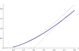
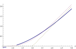
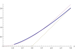
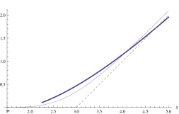
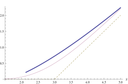
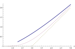
Figure 1: The solution $C_{a}(S,t)$ (thick line) of the generalized Black-Scholes equation versus the solution $C_{\rm call}(S,t)$ (thin line) of the Black-Scholes equation and the payoff function $C_{\rm call}(S,T)$ (dashed line) for $t=3$ (left hand side), $t=4$ (right hand side) and $a=-0.03$ (first row), $a=-0.02$ (second row), $a=-0.01$ (third row).

4 Concluding remarks

In quantum mechanics as well as in econophysics, exact solutions are known only in a small number of particular cases and, generally, they play an important role. The generalized version of the Black-Scholes equation investigated in this article:

- is exactly solvable for any $a\!\in\!(-\infty,0)$,

- satisfies the martingale condition for any $a\!\in\!(-\infty,0)$,

- coincides with the Black-Scholes equation in the limit case $a\nearrow 0$.
In practice, there are some deviations of prices from those described by the solution of the Black-Scholes equation. We think that the solution of the generalized Black-Scholes equation might describe some observed prices, and the parameter $a$ might have a certain financial meaning.

References

- [1] B.E. Baaquie, Quantum Finance, Cambridge University Press, 2004.
- [2] F. Bagarello, A quantum statistical approach to simplified stock markets, Physics A 388 (2009) 4397.
- [3] F. Cooper, A. Khare, U. Sukhatme, Supersymmetry and quantum mechanics, Phys. Rep. 251 (1995) 267.
- [4] L.-A. Cotfas, A finite-dimensional quantum model for the stock market, Physics A 392 (2013) 371.
- [5] N. Cotfas and L.A. Cotfas, Hypergeometric type operators and their supersymmetric partners, J. Math. Phys. 52 (2011) 052101.
- [6] M.A. Jafarizadeh and H. Fakhri, Parasupersymmetry and shape invariance in differential equations of mathematical physics and quantum mechanics, Ann. Phys. NY 262 (1998) 260.
- [7] T.K. Jana and P. Roy, Supersymmetry in option pricing, Physica A 390 (2011) 2350-55.
- [8] Ö. Uǧur, An Introduction to Computational Finance, Imperial College Press, London, 2009.