Formulas for Rational-Valued Separability Probabilities of Random Induced Generalized Two-Qubit States

Abstract

Previously, a formula, incorporating a $5F4$ hypergeometric function, for the Hilbert-Schmidt-averaged determinantal moments $\left\langle\left|\rho^{PT}\right|^{n}\left|\rho\right|^{k}\right\rangle/\left\langle\left|\rho\right|^{k}\right\rangle$ of $4\times 4$ density-matrices ($\rho$), and their partial transposes ($\rho^{PT}|$) was applied with $k=0$ to the generalized two-qubit separability-probability question. The formula can, further, be viewed we note here, as an averaging over “induced measures in the space of mixed quantum states”. The associated induced-measure separability probabilities ($k=1,2,\ldots$) are found–via a high-precision density approximation procedure–to assume interesting, relatively simple rational values in the two-re[al]bit ($\alpha=\frac{1}{2}$), (standard) two-qubit ($\alpha=1$) and two-quater[nionic]bit ($\alpha=2$) cases. We deduce rather simple companion (rebit, qubit, quaterbit,…) formulas that successfully reproduce the rational values assumed for general $k$. These formulas are observed to share certain features, possibly allowing them to be incorporated into a single master formula.

I Introduction

The question of the probability that a generic quantum system is separable/disentangled was raised in a 1998 paper of Życzkowski, Sanpera, Lewenstein and Horodecki, entitled ”Volume of the set of separable states” Życzkowski et al. (1998). Certainly, any particular answer to this question will crucially depend upon the measure that is attached to the systems in question. A large body of literature has arisen from the 1998 study, and we seek to make a significant contribution to it, addressing heretofore unsolved problems. Let us point out the work of Aubrun, Szarek and Ye Aubrun et al. (2014), which addresses questions of a somewhat similar nature to those examined below, while employing the same class of measures. However, their work is set in an asymptotic framework, while we will be concerned with obtaining exact finite-dimensional results (cf. Bhosale et al. (2012)). On the other hand, Singh, Kunjwal and Simon Singh et al. (2014) did focus on finite-dimensional scenarios, but with a distinct form of measure, the one originally used in Życzkowski et al. (1998).

We have investigated the possibility of extending to the class of ”induced measures in the space of mixed quantum states” Życzkowski and Sommers (2001); Bengtsson and Życzkowski (2006) the line of analysis reported in Slater and Dunkl (2012); Slater (2013), the principal separability probability findings of which–most notably the two-qubit conjecture of $\frac{8}{33}\approx 0.242424$–have recently been robustly supported, with the use of extensive Monte-Carlo sampling, by Fei and Joynt Fei and Joynt , as well as by Milz and Strunz, to somewhat similar effect (Milz and Strunz, 2015, Fig. 4, eqs. (30), (31)) (cf. (Khvedelidzea and Rogojina, 2013, Table 1)). This earlier line of work pertained to the use of the Hilbert-Schmidt measure (the particular symmetric case, $K=N$, of the induced measures) on the high-dimensional convex sets of generalized (real-, complex-, quaternionic-entried) two-qubit $(N=4$) states.

In (Slater and Dunkl, 2012, p. 30), a central role had been played by the (not yet formally proven) determinantal moment formula obtained there

$$\left\langle\left|\rho^{PT}\right|^{n}\left|\rho\right|^{k}\right\rangle/\left\langle\left|\rho\right|^{k}\right\rangle$$

$$=\frac{\left(k+1\right)_{n}\left(k+1+\alpha\right)_{n}\left(k+1+2\alpha\right)_{n}}{2^{6n}\left(k+3\alpha+\frac{3}{2}\right)_{n}\left(2k+6\alpha+\frac{5}{2}\right)_{2n}}$$

$$\cdot~{}_{5}F_{4}\left(\genfrac{}{}{0.0pt}{}{-n,-k,\alpha,\alpha+\frac{1}{2},-2k-2n-1-5\alpha}{-k-n-\alpha,-k-n-2\alpha,-\frac{k+n}{2},-\frac{k+n-1}{2}};1\right)$$

on the basis of extensive computations. Here $\rho^{PT}$ denotes the partial transpose Peres (1996) of the density matrix $\rho$, and $|\rho|$, its determinant, and generalized hypergeometric function notation is employed. The brackets represent averaging with respect to Hilbert-Schmidt measure Życzkowski and Sommers (2003). Furthermore, $\alpha$ is a random-matrix Dyson-index-like parameter Dumitriu and Edelman (2002), assuming, in particular, the value 1 for the standard (fifteen-dimensional convex set of) density matrices with complex-valued off-diagonal entries.

It subsequently occurred to us that this hypergeometric-based moment formula could be readily adapted to the broader class of random induced measures by considering, in the notation of Życzkowski and Sommers (2001); Bengtsson and Życzkowski (2006) that

$$k=K-N,$$ (1)

where $K$ is the dimension of the ancilla/environment state, over which the tracing operation is performed.

As in the earlier work Slater and Dunkl (2012); Slater (2013), a high-precision density-approximation (inverse) procedure of Provost, incorporating the first 11,401 such determinantal moments, strongly indicates that the random induced-measure separability probabilities ($k=1,2,\ldots$) assume interesting, relatively simple rational values in the two-re[al]bit ($\alpha=\frac{1}{2}$), (standard) two-qubit ($\alpha=1$) and two-quater[nionic]bit ($\alpha=2$) cases, particularly so for $\alpha=1$ (sec. II). One striking example is that for $k=3$, the $\alpha=1$ separability probability is found to be $\frac{27}{38}=\frac{3^{3}}{2\cdot 19}$ (to fifteen decimal places). In fact, based on extensive calculations ($k=0,\ldots,15,\ldots$) of this nature, we are able to deduce rather simple companion (rebit, qubit, quaterbit) formulas (2)-(4) that successfully reproduce the rational values assumed for general integer and half-integer $k$ (sec. III).

Further efforts along these lines have been given in a subsequent paper Slater , in which the determinantal inequality $|\rho^{PT}|>|\rho|$ is now imposed, rather than the broader inequality $|\rho^{PT}|>0$. (Of course, $|\rho|\geq 0$, while $|\rho^{PT}|$ is both a necessary and sufficient condition for separability here Peres (1996); Horodecki et al. (1996).) There, equivalent hypergeometric- and difference-equation-based formulas, $Q(k,\alpha)=G_{1}^{k}(\alpha)G_{2}^{k}(\alpha)$, for $k=-1,0,1,\ldots,9$, were given for that (rational-valued) portion of the total separability probability satisfying the stricter inequality. (We also preliminarily investigate this problem below in sec. IV.)

Milz and Strunz Milz and Strunz (2015) have recently reported a highly interesting finding that the conjectured Hilbert-Schmidt separability probability of $\frac{8}{33}\approx 0.242424$ holds constant along the radius of the Bloch sphere of either of the reduced subsystems of generic two-qubit ($\alpha=1$) systems. We are presently investigating the nature that the separability probability takes as a joint function of the radii of the two single-qubit subsystems, and related questions.

II Analysis

We pursue the indicated extension of our earlier (Hilbert-Schmidt-based) work to random induced measures, in general. As in Slater and Dunkl (2012); Slater (2013), the determinantal moment formula above is employed in the Legendre-polynomial-based (Mathematica-implemented) density approximation (inverse) procedure of Provost Provost (2005). This possesses a least-squares rationale. The program as originally presented is speeded, by incorporating the well-known recursion formula for Legendre polynomials, so that successive polynomials do not have to be computed ab initio. The computations are all exact, in nature, rather than numerical. Provost advises that the procedure should be regarded as an ”approximation”, rather than an ”estimation” scheme Provost (2005). (Let us note that the implementation of the procedure requires considerable caution and an adaptive strategy when the term $(k-j+1)_{n-j}$ (Slater and Dunkl, 2012, sec. D.2) in the underlying summation formula for the hypergeometric-based determinantal moments is zero. It is zero if $k-j+1\leq 0\leq k+n-2j$, that is, if values $j$ for which $k+1\leq j$ and $2j\leq k+n$ occur in the summation $j=0...n$.)

Now, with the use of an unprecedentedly large number (11,401) of the determinantal moments, we found (to ten decimal places) for $k=1$, the separability probability of the standard, complex ($\alpha=1$) 15-dimensional convex set of two-qubit states to be $\frac{61}{143}=\frac{61}{11\cdot 13}\approx 0.4265734$. On the other hand, for the Hilbert-Schmidt case ($k=K-N=0$), a very compelling body of evidence of a number of types (though yet no formal proof) has been adduced that the corresponding separability probability, as has been already noted, is $\frac{8}{33}=\frac{2^{3}}{3\cdot 11}\approx 0.242424$ Slater and Dunkl (2012); Slater (2013); Fei and Joynt ; Milz and Strunz (2015).

For the quaternionic ($\alpha=2$) case, the induced-measure ($k=1$) separability probability (now to thirteen decimal places) was $\frac{3736}{22287}=\frac{2^{3}\cdot 467}{3\cdot 17\cdot 19\cdot 23}\approx 0.16763135$, while the Hilbert-Schmidt counterpart strongly appears to be $\frac{26}{323}=\frac{2\cdot 13}{17\cdot 19}\approx 0.0804953$ Slater and Dunkl (2012); Slater (2013); Fei and Joynt .

Let us further note, though any immediate quantum-mechanical random-matrix division-algebra interpretation does not seem at hand, that for $k=1,\alpha=3$, we obtain a ”separability-probability” approximant, based on the 11,401 moments, that, to a remarkable sixteen decimal places equalled $\frac{8159}{124062}=\frac{41\cdot 199}{2\cdot 3\cdot 23\cdot 29\cdot 31}\approx 0.0657655$. This particularly high accuracy appears to essentially be an artifact of the Legendre-polynomial-based procedure that commences with a uniform distribution over the the interval $|\rho|\in[-\frac{1}{16},\frac{1}{256}]$. For such a distribution, the probability over the ”separability” interval of $[0,\frac{1}{256}]$ is the ratio of $\frac{1}{256}$ to $(\frac{1}{16}+\frac{1}{256})$, that is $\frac{1}{17}\approx 0.0588235$, quite near to 0.0657655. So as separability probability approximants increasingly deviate from the uniform-based one of $\frac{1}{17}$, at least for specific $k$, we can expect convergence of the density-approximation procedure to relatively weaken.

For the two-rebit scenario ($\alpha=\frac{1}{2}$), the associated Hilbert-Schmidt separability probability strongly appears to be $\frac{29}{64}=\frac{29}{2^{6}}\approx 0.453125$ Slater and Dunkl (2012); Slater (2013), while in the random induced-measure $k=1$ counterpart, we obtain (to almost nine decimal places) a value once again larger than that for the Hilbert-Schmidt case of $k=0$, that is, $\frac{515}{768}=\frac{5\cdot 103}{2^{8}\cdot 3}\approx 0.670573$. (Note the powers of 2, in both denominators–a phenomenon that will continue to be observed for rebit-related results.)

Table 1: Two-Rebit ($\alpha=\frac{1}{2}$) Separability Probabilities

$k=0$	$\frac{29}{64}$	$\frac{29}{2^{6}}$	0.453125
$k=1$	$\frac{515}{768}$	$\frac{5\cdot 103}{2^{8}\cdot 3}$	0.670573
$k=2$	$\frac{1645}{2048}$	$\frac{5\cdot 7\cdot 47}{2^{11}}$	0.803222
$k=3$	$\frac{31641}{35840}$	$\frac{3\cdot 53\cdot 199}{2^{10}\cdot 5\cdot 7}$	0.882840
$k=4$	$\frac{274373}{294912}$	$\frac{11\cdot 24943}{2^{15}\cdot 3^{2}}$	0.930355
$k=5$	$\frac{439777}{458752}$	$\frac{13\cdot 33829}{2^{16}\cdot 7}$	0.958638
$k=6$	$\frac{11251151}{11534336}$	$\frac{11251151}{2^{20}\cdot 11}$	0.975448
$k=7$	$\frac{30224045}{30670848}$	$\frac{5\cdot 17\cdot 53\cdot 6709}{2^{18}\cdot 3^{2}\cdot 13}$	0.985432
$k=8$	$\frac{10395147}{10485760}$	$\frac{3\cdot 7\cdot 19\cdot 26053}{2^{21}\cdot 5}$	0.991358

Table 2: Two-Qubit ($\alpha=1$) Separability Probabilities

$k=0$	$\frac{8}{33}$	$\frac{2^{3}}{3\cdot 11}$	0.242424
$k=1$	$\frac{61}{143}$	$\frac{61}{11\cdot 13}$	0.426573
$k=2$	$\frac{259}{442}$	$\frac{7\cdot 37}{2\cdot 13\cdot 17}$	0.585973
$k=3$	$\frac{27}{38}$	$\frac{3^{3}}{2\cdot 19}$	0.710526
$k=4$	$\frac{5960}{7429}$	$\frac{2^{3}\cdot 5\cdot 149}{17\cdot 19\cdot 23}$	0.802261
$k=5$	$\frac{379}{437}$	$\frac{379}{19\cdot 23}$	0.867277
$k=6$	$\frac{63881}{70035}$	$\frac{127\cdot 503}{3\cdot 5\cdot 7\cdot 23\cdot 29}$	0.912129
$k=7$	$\frac{1169237}{1240620}$	$\frac{37\cdot 31601}{2^{2}\cdot 3\cdot 5\cdot 23\cdot 29\cdot 31}$	0.942461
$k=8$	$\frac{25963}{26970}$	$\frac{7\cdot 3709}{2\cdot 3\cdot 5\cdot 29\cdot 31}$	0.962662

Table 3: Two-Quaterbit ($\alpha=2$) Separability Probabilities

$k=0$	$\frac{26}{323}$	$\frac{2\cdot 13}{17\cdot 19}$	0.080495
$k=1$	$\frac{3736}{22287}$	$\frac{2^{3}\cdot 467}{3\cdot 17\cdot 19\cdot 23}$	0.167631
$k=2$	$\frac{1807}{6555}$	$\frac{13\cdot 139}{3\cdot 5\cdot 19\cdot 23}$	0.275667
$k=3$	$\frac{3919}{10005}$	$\frac{3919}{3\cdot 5\cdot 23\cdot 29}$	0.391704
$k=4$	$\frac{104379}{206770}$	$\frac{3\cdot 11\cdot 3163}{2\cdot 5\cdot 23\cdot 29\cdot 31}$	0.504807
$k=5$	$\frac{16387}{26970}$	$\frac{7\cdot 2341}{2\cdot 3\cdot 5\cdot 29\cdot 31}$	0.607601
$k=6$	$\frac{69475}{99789}$	$\frac{5^{2}\cdot 7\cdot 397}{3\cdot 29\cdot 31\cdot 37}$	0.696219
$k=7$	$\frac{203123}{263958}$	$\frac{229\cdot 887}{2\cdot 3\cdot 29\cdot 37\cdot 41}$	0.769527
$k=8$	$\frac{1674746}{2022161}$	$\frac{2\cdot 837373}{31\cdot 37\cdot 41\cdot 43}$	0.828196

In Tables I, II and III, we present our conclusions, based on such high-precision calculations, as to the rational values ($k=0,1,\ldots 8$) assumed by these induced-measure separability probabilities. Let us note that with the sole exception of $k=7$, the rational values assumed by the (standard) two-qubit ($\alpha=1$) induced states have both smaller denominators and numerators than the other two cases tabulated, indicative, presumably, in some manner, of their greater ”naturalness”.

III Three Companion Separability Probability Formulas

Further extending the entries of the two-qubit table (Table II), but not explicitly showing the results here, to $k=17$, application of the Mathematica command FindSequenceFunction to the sequence of length eighteen obtained, plus subsequent simplification procedures, yielded the governing rule

$$P^{qubit}_{k}=1-\frac{3\ 4^{k+3}(2k(k+7)+25)\Gamma\left(k+\frac{7}{2}\right)\Gamma(2k+9)}{\sqrt{\pi}\Gamma(3k+13)}.$$ (2)

Here $P^{qubit}_{k}$ is the separability probability of the (15-dimensional) standard, complex two-qubit systems endowed with the induced measure $k=K-4$. This formula, thus, successfully reproduces the entries of Table II, as well as the subsequent ones ($k=9,\ldots,17$) we have approximated to high precision, making use of the 11,401 moments in the Provost Legendre-polynomial-based algorithm. (For $k=0$, formula (2) does, in fact, yield the apparent Hilbert-Schmidt separability probability of $\frac{8}{33}$ Slater and Dunkl (2012); Slater (2013); Fei and Joynt [Table II].)

Similarly, employing a somewhat longer sequence $k=0,\ldots,21$, we obtained the quaternionic ($\alpha=2$) counterpart

$$P^{quaterbit}_{k}=1-\frac{4^{k+6}(k(k(2k(k+21)+355)+1452)+2430)\Gamma\left(k+\frac{13}{2}\right)\Gamma(2k+15)}{3\sqrt{\pi}\Gamma(3k+22)},$$ (3)

yielding the $k=0$ (Hilbert-Schmidt) value of $\frac{26}{323}$. Further, for the rebit ($\alpha=\frac{1}{2}$) scenario, making analogous use of the sequence $k=0,\ldots,15$, we found

$$P^{rebit}_{k}=1-\frac{4^{k+1}(8k+15)\Gamma(k+2)\Gamma\left(2k+\frac{9}{2}\right)}{\sqrt{\pi}\Gamma(3k+7)},$$ (4)

yielding for $k=0$, the result $\frac{29}{64}$.

In Fig. 1 we show a joint plot of these three separability probability formulas, with the rebit one ($\alpha=\frac{1}{2}$) dominating the qubit one ($\alpha=1$), which in turn dominates the quaterbit ($\alpha=2$) curve.

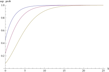
Figure 1: Two-rebit $>$ two-qubit $>$ two-quaterbit separability probabilities–given by (4), (2) and (3), respectively–as functions of $k=K-4$

In the limit $k\rightarrow\infty$, the three curves/probabilities all approach 1 (cf. Aubrun et al. (2014)). We have found (Slater, , sec. III)–through analytic means–that for each of $\alpha=1,2,3,4$ and $\frac{1}{2},\frac{3}{2},\frac{5}{2},\frac{9}{2}$, that as $k\rightarrow\infty$, the ratio of the logarithm of the $(k+1)$-st separability probability to the logarithm of the $k$-th separability probability is $\frac{16}{27}$. (Presumably, the pattern continues for larger $\alpha$, but the required computations have, so far, proved too challenging.)

It is interesting to observe, additionally, that for $k=-1$ (that is, $K=3$), a value not apparently susceptible to use of the principal $5F4$-hypergeometric determinantal moment formula and the density approximation (inverse) procedure of Provost Provost (2005), the three basic formulas yield the (now smaller than Hilbert-Schmidt) further simple rational values $\frac{1}{8},\frac{1}{14}$ and $\frac{11}{442}$, for the rebit, qubit and quaterbit cases, respectively (cf. (Aubrun et al., 2014, p. 130)). Further, for $k=-2$ $(K=2)$, the rebit formula has a singularity, the qubit formula yields 0, and the quaterbit one gives $\frac{1}{429}=\frac{1}{3\times 11\times 13}\approx 0.002331$.

We have been able to formally extend this series of three formulas to other values of $\alpha$, as well, including $\alpha=\frac{3}{2},\frac{5}{2},3,\frac{7}{2},4,\frac{9}{2},5,6,\ldots,13$ obtaining similarly structured (increasingly larger) formulas. A major challenge that we are continuing to address is to find a single master formula that encompasses these several results, and can itself yield the formula for any specific half-integer or integer value of $\alpha$ (Appendix I).

IV Division of Separability Probabilities Based on Determinantal Inequalities

We have also begun to investigate related aspects of the geometry of random-induced generalized two-qubit states, making use of a second hypergeometric-based determinantal moment formula (Slater and Dunkl, 2015, sec. II)

$$\left\langle\left|\rho\right|^{k}\left(\left|\rho^{PT}\right|-\left|\rho\right|\right)^{n}\right\rangle/\left\langle\left|\rho\right|^{k}\right\rangle =\left(-1\right)^{n}\frac{\left(\alpha\right)_{n}\left(\alpha+\frac{1}{2}\right)_{n}\left(n+2k+2+5\alpha\right)_{n}}{2^{4n}\left(k+3\alpha+\frac{3}{2}\right)_{n}\left(2k+6\alpha+\frac{5}{2}\right)_{2n}}$$

$$\times~{}_{4}F_{3}\left(\genfrac{}{}{0.0pt}{}{-\frac{n}{2},\frac{1-n}{2},k+1+\alpha,k+1+2\alpha}{1-n-\alpha,\frac{1}{2}-n-\alpha,n+2k+2+5\alpha};1\right).$$

The range of the determinant difference variable $(|\rho^{PT}|-|\rho|)$ is $[-\frac{1}{16},\frac{1}{432}]$, and we shall approximate the contributions over $[0,\frac{1}{432}]$ to the total separability probabilities given in Tables I, II and III.

In Slater and Dunkl (2015), employing the first 9,451 of these moments (having set $k$ to zero) in the density approximation procedure of Provost Provost (2005), we obtained highly convincing numerical evidence that the basic set of three Hilbert-Schmidt separability probabilities ($\frac{29}{64},\frac{8}{33},\frac{26}{323}$) was evenly (symmetrically) split (that is, $\frac{29}{128},\frac{4}{33},\frac{13}{323}$) between the two scenarios $|\rho^{PT}|>|\rho|$ and $|\rho|>|\rho^{PT}|>0$. Now, with the use of 14,051 such determinantal moments, with $k=1$, $\alpha=1$, we obtained an approximant equal to eight decimal places to $\frac{45}{286}=\frac{3^{2}\cdot 5}{2\cdot 11\cdot 13}\approx 0.157342657$ for the case $|\rho^{PT}|>|\rho|$. Employing the total separability probability $k=1$ result of $\frac{61}{143}$ in Table II, we find a complementary (larger) approximant of $\frac{7}{26}=\frac{7}{2\cdot 13}\approx 0.269230769$. So, the symmetry present in the Hilbert-Schmidt case (for example, $\frac{8}{33}=\frac{4}{33}+\frac{4}{33}$) is lost for $k\neq 0$.

Similarly, for the $k=1$, $\alpha=2$ counterpart, we obtain an approximant equal, to almost twelve decimal places, to $\frac{2056}{37145}=\frac{2^{3}\cdot 257}{5\cdot 17\cdot 19\cdot 23}\approx 0.0553506528470$, when $|\rho^{PT}|>|\rho|$, and, thus, $\frac{32}{285}=\frac{2^{5}}{3\cdot 5\cdot 19}\approx 0.1122807017544$ for the complementary (larger) approximant.

To complete the basic triad, that is $k=1$ and $\alpha=\frac{1}{2}$ (for which, convergence is typically weakest), for $|\rho^{PT}|>|\rho|$, we have an approximant equal, to more than six decimal places, to $\frac{281}{1024}=\frac{281}{2^{10}}\approx 0.2744140625$, and a complementary (larger, again) approximant of $\frac{1217}{3072}=\frac{1217}{2^{10}\cdot 3}\approx 0.3961588542$. (Note, again, the occurrence of powers of 2 in the $\alpha=\frac{1}{2}$ case.)

For $k=-1$, $\alpha=2$ it is interesting to note that the approximation of the probability $|\rho^{PT}|>|\rho|$ is $\frac{11}{442}$ to ten decimal places. This is the same rational value we found above for the total separability probability. It, thus, appears that we can conclude that the complementary probability (that is, for $|\rho|>|\rho^{PT}|>0$) is now smaller, in fact, zero, in contrast to the $k=1$ case. The complementary probability also appears to be zero for the two companion cases of $k=-1$, $\alpha=1$ and $\alpha=\frac{1}{2}$.

In Figure 2, we show–based on numerical results using 9,201 moments–the proportion of the three basic total random induced separability probabilities (Tables I, II, III), as a function of $k$, accounted for by the region $|\rho^{PT}|>|\rho|$.

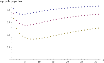
Figure 2: Proportion of the total random-induced separability probabilities–based on 9,201 moments–accounted for by the region $|\rho^{PT}|>|\rho|$. The two-rebit ($\alpha=\frac{1}{2}$) curve is dominant, the two-qubit ($\alpha=1$), intermediate, and the two-quaterbit ($\alpha=2$) curve, subordinate.

We have been investigating the possibility of obtaining explicit formulas–as we have been able to do above ((2),(3),(4)) for the total separability probabilities (that is, independently of whether $|\rho|>|\rho^{PT}|>0$ or $|\rho^{PT}|>|\rho|$)–for these sets of complementary probabilities. To even hope to achieve such a goal, it seems necessary to fill in considerably more rows of Table IV than we have so far been able to do (cf. Slater ).

V Alternative Density Approximation Procedure

In pursuit of such a goal, we have developed an alternative (Appendix II) to the Legendre-polynomial-based density approximation procedure of Provost Provost (2005), which we have made abundant use of above and in our earlier work Slater and Dunkl (2012); Slater (2013); Slater and Dunkl (2015). Though well-conditioned, it perhaps is relatively slow to converge for our purposes, since it takes as the baseline (starting) distribution, the uniform one, which is far from the sharply-peaked ones, with vanishing endpoints, we have encountered in our separability probability investigations. The approach outlined in Appendix II uses base functions of the form ${((x-a)(b-x))}^{\alpha}$ where $\alpha$ is a small positive integer. (Provost does present a number of codes, other than the Legendre-polynomial one, including one based on Jacobi polynomials (Provost, 2005, pp. 15, 24). It employs an adaptive strategy of matching the first and second given moments to those of a beta distribution. But we have found this algorithm to be highly ill-conditioned in our specific applications.)

VI Conclusions

We have reported above some considerable successes in our effort to extend to random induced measures Życzkowski and Sommers (2001); Bengtsson and Życzkowski (2006), earlier separability probability work Slater and Dunkl (2012); Slater (2013) based on the Hilbert-Schmidt measure (the particular symmetric $N=K$ case of the random induced measures), and the inequality $|\rho^{PT}|>0$. Further efforts using the more restrictive inequality $|\rho^{PT}]>|\rho|$ utilized in sec. IV have been given in a subsequent paper Slater . There equivalences between certain hypergeometric-based formulas and difference equations have been noted.

Let us importantly note that in the recent study Dunkl and Slater the (random induced measure) separability probability problems posed above, have, in fact, been exhaustively formally solved for the “toy” seven-dimensional $X$-states model Mendonça et al. (2014) of $4\times 4$ density matrices. Here, contrastingly, we have concentrated on the more general cases of $4\times 4$ density matrices with none of the off-diagonal entries a priori nullified (as they are in the $X$-states model). Although, we have developed certain formulas here, for which the evidentiary support is quite considerable, we still lack formal proofs in this higher-dimensional venue.

We continue to investigate these problems in search of a still more definitive (”master formula”) resolution of them (Appendix I). As a possible tool in such research, we have developed (Appendix II) an alternative density approximation procedure to that of Provost Provost (2005), on which we have strongly relied to this point in obtaining exact separability probability results.

Table 4: Proportions of total separability probabilities $|\rho^{PT}|>|\rho|$

$\alpha$	$\frac{1}{2}$	1	2
$k=0$	$\frac{1}{2}$	$\frac{1}{2}$	$\frac{1}{2}$
$k=1$	$\frac{843}{2060}$	$\frac{45}{122}$	$\frac{771}{2335}$
$k=2$	$\frac{9949}{26320}$	$\frac{1553}{4921}$	$\frac{26503}{104806}$
$k=3$	—	$\frac{3073}{10557}$	$\frac{51585}{242978}$
$k=4$	—	$\frac{2087}{7450}$	$\frac{2195945}{11586069}$
$k=5$	—	—	$\frac{4390079}{24859079}$
$k=6$	—	—	$\frac{8310451}{48993770}$

VII Appendix I. Master Formula Investigation

This appendix is based on the random induced measure separability probability formulas we have obtained for $\alpha=\frac{1}{2},\frac{3}{2},\frac{5}{2},\frac{7}{2},1,\ldots 13\vskip 6.0pt plus 2.0pt minus 2.0pt$.

The purpose is to find $P\left\{\left|\rho^{PT}\right|>0\right\}$ with respect to the normalized measure $\left|\rho\right|^{k}$ with parameter $\alpha$. The values $\alpha=\frac{1}{2},1,2$ correspond to the real, complex, quaternion cases respectively. The obtained formulas have the form

$$P\left\{\left|\rho^{PT}\right|>0\right\}=1-F\left(\alpha,k\right).$$

Define

$$G\left(\alpha,k\right):=4^{k}\frac{\Gamma\left(k+3\alpha+\frac{3}{2}\right)\Gamma\left(2k+5\alpha+2\right)}{\Gamma\left(\frac{1}{2}\right)\Gamma\left(3k+10\alpha+2\right)}.$$

The first observation: when $\alpha$ is integer or half-integer $\dfrac{F\left(\alpha,k\right)}{G\left(\alpha,k\right)}$ is a rational function of $k$, that is, a ratio of polynomials.

The second observation: when $\alpha$ is an integer then

$$F\left(\alpha,k\right)=p_{\alpha}\left(k\right)G\left(\alpha,k\right),$$

where $p_{\alpha}\left(k\right)$ is a polynomial of degree $4\alpha-2$ with leading coefficient $\dfrac{2^{8\alpha+1}}{\left(2\alpha-1\right)!},$ and $p_{\alpha}$ can be factored as $\left(k+g_{1}\left(\alpha\right)\right)\left(k+g_{1}\left(\alpha\right)+1\right)\cdots\left(k+g_{2}\left(\alpha\right)\right)\widetilde{p_{\alpha}}\left(k\right)$, where $\widetilde{p_{\alpha}}\left(k\right)$ is irreducible in general; furthermore

$$g_{1}\left(\alpha\right) :=2\alpha+1+\left\lfloor\frac{\alpha+1}{2}\right\rfloor,$$

$$g_{2}\left(\alpha\right) :=3\alpha+\left\lfloor\frac{\alpha+1}{3}\right\rfloor.$$

The sequence of values $\left[g_{1}\left(\alpha\right),g_{2}\left(\alpha\right)\right]$ for $\alpha=2,\ldots,14$ is

$$\left[6,7\right],[9,10],[11,13],[14,17],[16,20],[19,23],[21,27],[24,30],[26,33],[29,37],$$

$$[31,40],[34,43],[36,47]$$

These conjectures imply that the degree of $\widetilde{p_{\alpha}}\left(k\right)$ is

$$4\alpha-2-\left(g_{2}\left(\alpha\right)+1-g_{1}\left(\alpha\right)\right)=3\alpha+\left\lfloor\frac{\alpha+1}{2}\right\rfloor-\left\lfloor\frac{\alpha+1}{3}\right\rfloor-2.$$

The coefficient of $k^{4\alpha-3}$ in $\left(\frac{2^{8\alpha+1}}{\left(2\alpha-1\right)!}\right)^{-1}p_{\alpha}\left(k\right)$ (note that this is monic, coefficient of $k^{4\alpha-2}$ is $1$) is given by

$$c_{2}\left(\alpha\right):=-3+\frac{3}{2}\alpha+\frac{17}{2}\alpha^{2}+\left(\left\lfloor\frac{\alpha-1}{4}\right\rfloor-\left\lfloor\frac{\alpha}{4}\right\rfloor\right)\left(1+\frac{5}{2}\alpha\right),$$

equivalently

$$c_{2}\left(\alpha\right)=\left\{\begin{array}[c]{c}-4-\alpha+\frac{17}{2}\alpha^{2},\alpha\equiv 0\operatorname{mod}4,\\ -3+\frac{3}{2}\alpha+\frac{17}{2}\alpha^{2},\alpha\neq 0\operatorname{mod}4.\end{array}\right.$$

To determine the second coefficient of $\widetilde{p_{\alpha}}$ note that the second coefficient of $\left(k^{n}+a_{2}k^{n-1}+\ldots\right)\left(k^{m}+b_{2}k^{m-1}+\ldots\right)=k^{n+m}+\left(a_{2}+b_{2}\right)k^{n+m-1}+\ldots$ is $a_{2}+b_{2}$, so the second coefficient of $\left(k+g_{1}\left(\alpha\right)\right)\left(k+g_{1}\left(\alpha\right)+1\right)\cdots\left(k+g_{2}\left(\alpha\right)\right)$ is subtracted from $c_{2}\left(\alpha\right)$. This coefficient is

$$c_{2}^{\prime}\left(\alpha\right) :=\sum_{i=g_{1}\left(\alpha\right)}^{g_{2}\left(\alpha\right)}i=\frac{1}{2}\left(g_{1}\left(\alpha\right)+g_{2}\left(\alpha\right)\right)\left(g_{2}\left(\alpha\right)-g_{1}\left(\alpha\right)+1\right)$$

$$=\frac{1}{2}\left(5\alpha+1+\left\lfloor\frac{\alpha+1}{2}\right\rfloor+\left\lfloor\frac{\alpha+1}{3}\right\rfloor\right)\left(\alpha+\left\lfloor\frac{\alpha+1}{3}\right\rfloor-\left\lfloor\frac{\alpha+1}{2}\right\rfloor\right).$$

The second coefficient of $\widetilde{p_{\alpha}}$ is $c_{2}\left(\alpha\right)-c_{2}^{\prime}\left(\alpha\right)$; the sequence of values for $\alpha=1\ldots 14$ is

$$[7,21,59,92,155,222,319,364,510,626,745,853,1068,1186].$$

Denote the coefficient of $k^{4\alpha-4}$ in $\left(\frac{2^{8\alpha+1}}{\left(2\alpha-1\right)!}\right)^{-1}p_{\alpha}\left(k\right)$ by $c_{3}\left(\alpha\right)$ then from the calculated values ($\alpha=1,\ldots,13$) we find for $\alpha\neq 0\operatorname{mod}4$ that

$$c_{3}\left(\alpha\right)=11-\frac{389}{24}\alpha-\frac{333}{16}\alpha^{2}+\frac{115}{48}\alpha^{3}+\frac{289}{8}\alpha^{4}.$$

The third observation: when $\alpha$ is a half-integer then

$$F\left(\alpha,k\right)=\frac{p_{\alpha}\left(k\right)}{\left(k+2\alpha+1\right)_{\alpha+1/2}}G\left(\alpha,k\right),$$

where $p_{\alpha}\left(k\right)$ is a polynomial of degree $5\alpha-\frac{3}{2}$ with leading coefficient $\dfrac{2^{8\alpha+1}}{\left(2\alpha-1\right)!}$.

VIII Appendix II. A modification of the Provost-Legendre method using Gegenbauer polynomials

We consider the problem of approximating a density function with given moments using Jacobi polynomials for some choice of parameters. The technique uses a construction of Provost (Provost, 2005, sec. 4) which is adapted for a specific aspect of the unknown probability density, namely, $\Pr\left\{X>0\right\}$.

Suppose the density $f\left(x\right)$ is supported on the interval $\left[a,b\right]$ with given (i.e. computable) moments $\mu_{n}:=\int_{a}^{b}x^{n}f\left(x\right)dx$, and $\left\{p_{n}\left(x\right)\right\}$ is a family of orthogonal polynomials with weight function $w\left(x\right)$ also on $\left[a,b\right]$; the structure constants are

$$h_{n}:=\int_{a}^{b}p_{n}\left(x\right)^{2}w\left(x\right)dx,~{}n=0,1,2,\ldots$$

The aim is to (implicitly) determine the expansion

$$f\left(x\right)=\sum_{n=0}^{\infty}\lambda_{n}p_{n}\left(x\right)w\left(x\right).$$

and to apply it to the approximation of (where $a<0<b$)

$$\Pr\left\{X>0\right\}=\int_{0}^{b}f\left(x\right)dx=\sum_{n=0}^{\infty}\lambda_{n}\int_{0}^{b}p_{n}\left(x\right)w\left(x\right)dx.$$

By orthogonality, for $m=0,1,2,\ldots$

$$\int_{a}^{b}p_{m}\left(x\right)f\left(x\right)dx =\sum_{n=0}^{\infty}\lambda_{n}\int_{a}^{b}p_{n}\left(x\right)p_{m}\left(x\right)w\left(x\right)dx$$

$$=\lambda_{m}h_{m}.$$

To evaluate the left hand side compute the coefficients $\left\{a_{ni}:0\leq i\leq n\right\}$ in the expansions

$$p_{n}\left(x\right)=\sum_{i=0}^{n}a_{ni}x^{i},$$

when $\left\{p_{n}\left(x\right)\right\}$ are shifted Jacobi polynomials (this requires extra computation since the shortest expansions are in powers of $\left(x-a\right)$ or $\left(b-x\right)$); then

$$\lambda_{m}h_{m} =\int_{a}^{b}\sum_{i=0}^{m}a_{mi}x^{i}f\left(x\right)dx=\sum_{i=0}^{m}a_{mi}\mu_{i},$$

$$\lambda_{m} =\frac{1}{h_{m}}\sum_{i=0}^{m}a_{mi}\mu_{i};$$

The main problem is to approximate $\int_{\xi}^{b}f\left(x\right)dx$ for some given $\xi$: so

$$\int_{a}^{\xi}f\left(x\right)dx=\sum_{n=0}^{\infty}\lambda_{n}\int_{\xi}^{b}p_{n}\left(x\right)w\left(x\right)dx.$$

Compute

$$q_{n}:=\int_{\xi}^{b}p_{n}\left(x\right)w\left(x\right)dx,$$

then

$$\int_{\xi}^{b}f\left(x\right)dx =\sum_{n=0}^{\infty}\lambda_{n}q_{n}=\sum_{n=0}^{\infty}\frac{1}{h_{n}}\sum_{i=0}^{n}a_{ni}\mu_{i}q_{n}$$

$$=\sum_{i=0}^{\infty}\mu_{i}\sum_{n=i}^{\infty}\frac{q_{n}}{h_{n}}a_{ni},$$

and now we observe that the sum over $n$ is the coefficient of $x^{i}$ in

$$\sum_{n=0}^{\infty}\frac{q_{n}}{h_{n}}p_{n}\left(x\right).$$

Truncate the infinite series to obtain an approximation.

Jacobi polynomials: We start with background information about general parameters and then specialize to equal parameters. The family $\left\{P_{n}^{\left(\alpha,\beta\right)}\left(t\right)\right\}$ is orthogonal for $\left(1-t\right)^{\alpha}\left(1+t\right)^{\beta}$;

$$P_{n}^{\left(\alpha,\beta\right)}\left(t\right)=\frac{\left(\alpha+1\right)_{n}}{n!}~{}_{2}F_{1}\left(\genfrac{}{}{0.0pt}{}{-n,n+\alpha+\beta+1}{\alpha+1};\frac{1-t}{2}\right)$$

$$\frac{d}{dt}\left\{\left(1-t\right)^{\alpha+1}\left(1+t\right)^{\beta+1}P_{n-1}^{\left(\alpha+1,\beta+1\right)}\left(t\right)\right\}=-2n\left(1-t\right)^{\alpha}\left(1+t\right)^{\beta}P_{n}^{\left(\alpha,\beta\right)}\left(t\right)$$ (5)

$$h_{n}=2^{\alpha+\beta+1}B\left(\alpha+1,\beta+1\right)\frac{\left(\alpha+1\right)_{n}\left(\beta+1\right)_{n}\left(\ \alpha+\beta+n+1\right)}{n!\left(\alpha+\beta+2\right)_{n}\left(\ \alpha+\beta+2n+1\right)}.$$

Equation (5) is from (Olver et al., 2010, 18.9.16). To shift to the interval $\left[a,b\right]$ set

$$x =\frac{1}{2}\left(\left(b-a\right)t+a+b\right),~{}t=\frac{2x-a-b}{b-a}$$

$$w\left(x\right) =\left(\frac{2}{b-a}\right)^{\alpha+\beta+1}\left(b-x\right)^{\alpha}\left(x-a\right)^{\beta},$$

$$p_{n}\left(x\right) =P_{n}^{\left(\alpha,\beta\right)}\left(\frac{2x-a-b}{b-a}\right),$$

and the key quantities $q_{n}$ are found by

$$\int_{\xi}^{b}p_{n}\left(x\right)w\left(x\right)dx =\left(\frac{2}{b-a}\right)^{\alpha+\beta+1}\int_{\xi}^{b}P_{n}^{\left(\alpha,\beta\right)}\left(\frac{2x-a-b}{b-a}\right)\left(b-x\right)^{\alpha}\left(x-a\right)^{\beta}dx$$

$$=\int_{\zeta}^{1}P_{n}^{\left(\alpha,\beta\right)}\left(t\right)\left(1-t\right)^{\alpha}\left(1+t\right)^{\beta}dt$$

$$=-\frac{1}{2n}\int_{\zeta}^{1}\frac{d}{dt}\left\{\left(1-t\right)^{\alpha+1}\left(1+t\right)^{\beta+1}P_{n-1}^{\left(\alpha+1,\beta+1\right)}\left(t\right)\right\}dt$$

$$=\frac{1}{2n}\left(1-\zeta\right)^{\alpha+1}\left(1+\zeta\right)^{\beta+1}P_{n-1}^{\left(\alpha+1,\beta+1\right)}\left(\zeta\right),n\geq 1;$$

$$\zeta =\frac{2\xi-a-b}{b-a},$$

and $q_{0}=\int_{\zeta}^{1}\left(1-t\right)^{\alpha}\left(1+t\right)^{\beta}dt.$

In the case $a=-\frac{1}{16},b=\frac{1}{432}$, $\xi=0$ the transformations are

$$t =\frac{216}{7}x+\frac{13}{14},\zeta=\frac{13}{14},$$

$$p_{n}\left(x\right) =P_{n}^{\left(\alpha,\beta\right)}\left(\frac{216}{7}x+\frac{13}{14}\right).$$

Thus the strategy is to choose appropriate parameters $\alpha,\beta$ (small integer values appear to work well), then determine the coefficients of $\left\{x^{i}\right\}$ in the truncated series

$$\sum_{n=0}^{\infty}\frac{q_{n}}{h_{n}}P_{n}^{\left(\alpha,\beta\right)}\left(\frac{2x-a-b}{b-a}\right).$$

Computational details:

Given $\left[a,b\right]$ with $a<0<b$ let $c_{0}:=-\dfrac{a+b}{b-a}$, $c_{1}:=\dfrac{2}{b-a}$ and specialize to $\alpha=\beta=\lambda-\frac{1}{2}\geq 0$, so that the weight is $\left(1-t^{2}\right)^{\alpha}$ and the Gegenbauer polynomials $P_{n}^{\lambda}$ form the orthogonal basis. We use the normalized polynomials with $P_{n}^{\lambda}\left(1\right)=1$. (Note that $P_{n}^{\lambda}\left(t\right)=\frac{n!}{\left(\lambda+\frac{1}{2}\right)_{n}}P_{n}^{\left(\lambda-1/2,\lambda-1/2\right)}\left(t\right).)$ The recurrence is $P_{0}^{\lambda}\left(t\right)=1,P_{1}^{\lambda}\left(t\right)=t,$

$$P_{n+1}^{\lambda}\left(t\right)=\frac{2n+2\alpha+1}{n+2\alpha+1}tP_{n}^{\lambda}\left(t\right)-\frac{n}{n+2\alpha+1}P_{n-1}^{\lambda}\left(t\right),n\geq 1$$

and

$$h_{n}=\frac{\Gamma\left(\frac{1}{2}\right)\Gamma\left(\alpha+1\right)}{\Gamma\left(\alpha+\frac{3}{2}\right)}\frac{n!\left(2\alpha+1\right)}{\left(2\alpha+1\right)_{n}\left(2n+2\alpha+1\right)}=h_{0}\eta_{n},$$

where

$$\eta_{0}=1,\eta_{n}=\frac{n\left(2n+2\alpha-1\right)}{\left(2n+2\alpha+1\right)\left(n+2\alpha\right)}\eta_{n-1},n\geq 1.$$

(see (Dunkl and Xu, 2014, Sect. 1.4.3)). In the recurrence replace $t$ by $c_{0}+y$, where $y=c_{1}x$ (this takes the scaling factor out of the computations) Let

$$P_{n}^{\lambda}\left(c_{0}+y\right)=\sum_{j=0}^{n}B_{nj}y^{j},$$

then (with the convention $B_{n,-1}=0$)

$$B_{00} =1,~{}B_{1,0}=c_{0},~{}B_{1,1}=1,$$

$$B_{nj} =\frac{2n+2\alpha-1}{n+2\alpha}\left(c_{0}B_{n-1,j}+B_{n-1,j-1}\right)-\frac{n-1}{n+2\alpha}B_{n-2,j},~{}n\geq 2,~{}0\leq j\leq n.$$

Furthermore

$$\frac{d}{dt}\left\{\left(1-t^{2}\right)^{\alpha+1}P_{n-1}^{\lambda+1}\left(t\right)\right\}=-2\left(\alpha+1\right)\left(1-t^{2}\right)^{\alpha}P_{n}^{\lambda}\left(t\right),$$

$$q_{n}=\int_{c0}^{1}\left(1-t^{2}\right)^{\alpha}P_{n}^{\lambda}\left(t\right)dt=\frac{1}{2\left(\alpha+1\right)}\left(1-c_{0}^{2}\right)^{\alpha+1}P_{n-1}^{\lambda+1}\left(c_{0}\right),n\geq 1,$$

$$q_{0}=\int_{c_{0}}^{1}\left(1-t^{2}\right)^{\alpha}dt,$$

and $P_{n-1}^{\lambda+1}\left(c_{0}\right)=g_{n}$ can be computed with the recurrence

$$g_{1} =1,g_{2}=c_{0},$$

$$g_{n} =\frac{2n+2\alpha-1}{n+2\alpha+1}c_{0}g_{n-1}-\frac{n-2}{n+2\alpha+1}g_{n-2},$$

thus $q_{1}=\frac{1}{2\left(\alpha+1\right)}\left(1-c_{0}^{2}\right)^{\alpha+1}$ and $q_{n}=g_{n}q_{1}$. Note: if $\alpha$ and $c_{0}$ are rational then the quantities $\left\{B_{nj}\right\}$, $\left\{\eta_{n}\right\}$ and $\left\{g_{n}\right\}$ can be computed in exact arithmetic.

Suppose the process is terminated at some $m$, then (approximate values)

$$A_{0} =\frac{q_{0}}{h_{0}}+\frac{q_{1}}{h_{0}}\sum_{j=1}^{m}\frac{g_{j}}{\eta_{j}}B_{j,0}$$

$$A_{i} =c_{1}^{i}\frac{q_{1}}{h_{0}}\sum_{j=i}^{m}\frac{g_{j}}{\eta_{j}}B_{j,i},~{}1\leq i\leq m.$$

Since polynomial interpolation tends to be not numerically well-conditioned (a lot of cancellation) it is suggested to compute the quantities $\left\{q_{j}\right\},\left\{B_{j,i}\right\}$ to high precision, or even better, in exact arithmetic for $\alpha=0,1,2,\ldots$.

Conflict of Interests
The authors declare that there is no conflict of interests regarding the publication of this paper.