Distributions of positive signals in pyrosequencing

Abstract

Pyrosequencing is one of the important next-generation sequencing technologies. We derive the distribution of the number of positive signals in pyrograms of this sequencing technology as a function of flow cycle numbers and nucleotide probabilities of the target sequences. As for the distribution of sequence length, we also derive the distribution of positive signals for the fixed flow cycle model. Explicit formulas are derived for the mean and variance of the distributions. A simple result for the mean of the distribution is that the mean number of positive signals in a pyrogram is approximately twice the number of flow cycles, regardless of nucleotide probabilities. The statistical distributions will be useful for instrument and software development for pyrosequencing and other related platforms.

1 Introduction

The next-generation sequencing is transforming biological research in many aspects. Pyrosequencing is one of the important new sequencing platforms. Compared with other next-generation sequencing technologies, currently pyrosequencing has the advantage of longer sequence read length, which makes it possible for de novo sequencing of new genomes and other applications.

Pyrosequencing technology is based on detection of pyrophosphate (PPi) that is released during DNA synthesis. The four kinds of nucleotides (dATP, dCTP, dGTP, and dTTP) are added iteratively in a pre-defined order, with one kind of nucleotide at a time. For each nucleotide flow, if the nucleotide is complementary to the DNA template, the nucleotide is incorporated by polymerase. A detectable light is then emitted with an intensity which is in theory proportional to the number of incorporated nucleotides. If the added nucleotide is not complementary to the template, ideally no light signal is emitted. Because we know which nucleotide is added at each nucleotide flow, the DNA sequence of the template can be determined by the presence or absence of the emitted light and its intensity. The detected light signals are usually presented as a pyrogram (also called flowgram), in which the x-axis is the pre-determined nucleotide flows and y-axis is the intensity of the emitted light at each nucleotide flow. Thus the pyrogram consists of both positive and zero signals: positive signals correspond to the emitted light signals, which in turn reflect nucleotide incorporation activities, while zero signals correspond to background noise with no nucleotide incorporation. In a pyrogram the positive signals are interspersed with zero signals.

To avoid unnecessary specification of the detailed names of the four kinds of nucleotides, in the following we will use $a$, $b$, $c$, and $d$ to represent any permutations of the usual nucleotides $A$, $C$, $G$, and $T$. In Table 1 the relations between nucleotide flow, flow cycle number $f$, and the pyrogram of a sample sequence are shown. The sample sequence shown in Table 1 is

$$bddabaaad.$$ (1)

If flow order is {$a$-$b$-$c$-$d$}, the pyrogram of above sample sequence is {0-1-0-2}-{1-1-0-0}-{3-0-0-1}, or in short-hand notion

$$010211003001,$$ (2)

where non-zeros are the positive signals. In the first flow cycle ($f=1$), the first three nucleotides $bdd$ are synthesized to give out signals {0-1-0-2}, in the second flow cycle ($f=2$), the next two nucleotides $ab$ are synthesized to give out signals {1-1-0-0}, and in the third flow cycle ($f=3$), the remaining nucleotides $aaad$ are synthesized to give out signals {3-0-0-1}. If we represent the positive signals using the upper case letters of the corresponding nucleotide flow and ignore the zeros, we end up with the last row in Table 1:

$$BDABAD.$$ (3)

Sequence (3) represents the runs of the original Sequence (1), which we will call as r-seq of the original sequence. Here a run in a random sequence is defined as a stretch of consecutive identical element of one object separated by elements of other objects or the end of the sequence. The study of distributions of various runs has a long history and has found important applications in various fields (Balakrishnan and Koutras, 2002; Kong, 2006, 2013). It is obvious that for any given sequence such as Sequence (1), there is a unique corresponding r-seq, which is obtained by shrinking a stretch of consecutive identical letters (defined as a run) into a single letter. The reverse is however not true. In fact, there are infinite number of sequences that can have Sequence (3) as their r-seqs. The first $B$ in Sequence (3), for example, can come from $b$, $bb$, $bbb$, etc. The length of r-seq is clearly dependent on the context of the original sequence. For example, if we just shuffle Sequence (1) into another sequence

$$aaaabbddd,$$

the corresponding r-seq will be $ABD$.

Previously, we have studied the distribution of the sequence length (of the original sequences) for pyrosequencing as well as the more general case where nucleotide incorporation is probabilistic  (Kong, 2009a, b, 2012). In this paper, we are interested in the distribution of the length of r-seqs: what is the distribution of the number of the positive signals in a pyrogram, for a given number of flow cycles?

Table 1: The relation between nucleotide flow, flow cycle number $f$, the pyrogram of a sample sequence $bddabaaad$, and its corresponding positive signals.

Flow cycle	$f=1$				$f=2$				$f=3$
Nucleotide flow	$a$	$b$	$c$	$d$	$a$	$b$	$c$	$d$	$a$	$b$	$c$	$d$
Pyrogram	0	1	0	2	1	1	0	0	3	0	0	1
Positive signals		$B$		$D$	$A$	$B$			$A$			$D$

The distribution of the positive signals in a pyrogram (the length of r-seq), besides being an interesting self-contained mathematical problem, has important practical applications for algorithm and software development of the pyrosequencing technology. It has immediate implications for base-calling algorithms. Currently, base-callers for pyrosequencing use fixed pre-determined thresholds to call the presence or absence of any bases. Due to signal intensity variations and background noises, base-calling errors (insertions and deletions) are inevitable by using fixed thresholds. In fact, the higher amount of insertion and deletion errors made during base-calling step is a major drawback of pyrosequencing and similar sequencing technologies. The availability of the distribution of the positive signals in the pyrograms points to a potentially new direction for base-caller algorithm development for pyrosequencing. For example, one can envision that in a bootstrapping fashion, the thresholds used to call the bases can be iteratively adjusted based on the deviation of the number of positive signals obtained by these thresholds from the expected distribution, so that an optimal set of thresholds can be obtained that minimizes the difference. Another use of the theoretical distribution of positive signals is to test base independence. The distribution obtained in this paper is based on the assumption that the nucleotides in the target sequence are independent of each other. If the bases in the sequence are correlated, this assumption will be violated and the actual distribution of the sequence will not obey the theoretical distribution.

The development of this paper follows similar route we took to obtain the distribution of sequence length. First we study the situation where the number of positive signals is pre-defined as $r$. We term this as fixed r-seq length model (FRLM). This is analogous to the fixed sequence length model when the sequence length distributions were studied. Within this model we first develop proper recursive relations, then use generating functions (GFs) to solve these recursive relations. The GFs obtained then readily yield the mean and variance for the distribution. From FRLM then we transform to the more realistic fixed flow cycle model (FFCM), in which instead of fixing length of r-seq, we fix the number of flow cycles $f$ and treat $r$ as a random variable. This model is of more practical use. A simple and somewhat surprising result coming from the distribution of $r$ is that the mean of $r$ is approximately twice the number of flow cycles: $\bar{r}\approx 2f$ (Eq. (17a) for FRLM and Eq. (23a) for FFCM), regardless of nucleotide probabilities of the target sequences. In other words, on average in a pyrogram about half of the nucleotide flows has positive signals, and the other half has zero signal.

The GF approach not only gives the exact distributions and various moments of the distributions (with mean and variance as special cases), it also leads naturally to the limiting distributions (Flajolet and Sedgewick, 2009). All the distributions obtained previously from this series of work as well as those derived in this paper are asymptotically Gaussian, with the mean and variance linear with the size of the system.

The paper is organized as follows. First in the remaining of this Introduction section we define the necessary notation. Then we proceed to fixed r-seq length model (FRLM). There the recurrences and GF solution are presented. Explicit formulas are derived for the mean and variance of the distributions, for both fixed number of cycles and fixed number of positive signals. Based on results from FRLM we then obtain the results for FFCM. The analytical results of FFCM are carefully compared with the simulation results, which are posted. In the last section we summarize and discuss the results obtained so far for the pairwise relations between $f$ (flow cycle), $r$ (r-seq length), and $n$ (sequence length), and point out the non-transitive nature for the variances of these distributions. In this paper, we will only focus on the case of pyrosequencing, where the nucleotides are completely incorporated in each nucleotide flow. The case of incomplete nucleotide incorporation will be discussed elsewhere.

1.1 Notation and definitions

As stated earlier, we will use $a$, $b$, $c$, and $d$ to represent any permutations of the usual nucleotides $A$, $C$, $G$, and $T$. As shown in Sequence (3), the upper case letters $A$, $B$, $C$, and $D$ are used for the runs of nucleotides of the corresponding lower case letters. Throughout the paper we assume that the nucleotides in the target sequence are independent of each other. The probabilities for the four nucleotides in the target sequence are denoted as $p_{a}$, $p_{b}$, $p_{c}$, and $p_{d}$. In Table 1 we define the flow cycle number $f$ (the first row) to distinguish it from nucleotide flow cycle (the second row). A flow cycle is the “quad cycle” of successive four nucleotides {$abcd$}. The flow cycle number is denoted as $f$ in the following. We assume that the flow cycle $f$ is always a complete cycle (i.e., the number of nucleotide cycles is always a multiple of $4$). We will use $r$ for the number of positive signals in a pyrogram. It is identical to the total number of runs in the original sequence, or equivalently, the length of the corresponding r-seq (Kong, 2006, 2013). For example, the length of Sequence (3) is the total number of runs in the original Sequence (1), and is also the number of positive signals in the pyrogram (2) of the same sequence.

In the following we will frequently use the definition of elementary symmetric functions to express the results in more compact forms. For our purpose the elementary symmetric functions with four variables are defined in Eq. (4), in terms of the nucleotide probabilities:

$$\begin{aligned} e_{1}&=p_{a}+p_{b}+p_{c}+p_{d},\\ e_{2}&=p_{a}p_{b}+p_{a}p_{c}+p_{a}p_{d}+p_{b}p_{c}+p_{b}p_{d}+p_{c}p_{d},\\ e_{3}&=p_{a}p_{b}p_{c}+p_{a}p_{b}p_{d}+p_{a}p_{c}p_{d}+p_{b}p_{c}p_{d},\\ e_{4}&=p_{a}p_{b}p_{c}p_{d}.\end{aligned}$$ (4)

It’s obvious that we have the constraint on $e_{1}$ as $e_{1}=p_{a}+p_{b}+p_{c}+p_{d}=1$. We also need the following definition, which represents a value that is proportional to the probability of one positive signal of a particular nucleotide, with the number of nucleotides in the signal ranging from $1$ to infinity:

$$\mu_{i}=\sum_{j=1}^{\infty}p_{i}^{j}=\frac{p_{i}}{1-p_{i}},\qquad i=a,b,c,d.$$ (5)

We’ll frequently extract coefficients from the expansion of GFs. If $h(x)$ is a series in powers of $x$, then we use the notation $[x^{n}]h(x)$ to denote the coefficient of $x^{n}$ in the series. Similarly, we use $[x^{n}y^{m}]h(x,y)$ to denote the coefficient of $x^{n}y^{m}$ in the bivariate $h(x,y)$.

2 Fixed r-seq length model (FRLM)

In this model we assume that the number of positive signals $r$ is fixed. Let $L_{i}(f,r)$ ($i=a$, $b$, $c$, and $d$) denote the probability (up to a normalization factor, see below) that a r-seq of length $r$ and ending with nucleotide $i$ is synthesized in the first $f$ flow cycles, with the $r$-th positive signals synthesized in flow cycle $f$. Symbolically we can enumerate the first few terms for small $r$ as in Table 2.

Table 2: The first few terms for FRLM. Here $\mathcal{S}_{2}=AB+AC+BC+AD+BC+CD$. Note that non-zero terms of $r=3$ and $f=3$ are not shown: $CBA+DBA+DCA$ for nucleotide flow $a$, and $DCB$ for nucleotide flow $b$.

	$f=1$				$f=2$
$r$	$a$	$b$	$c$	$d$	$a$	$b$	$c$	$d$
$1$	$A$	$B$	$C$	$D$	$0$	$0$	$0$	$0$
$2$	0	$AB$	$(A+B)C$	$(A+B+C)D$	$(B+C+D)A$	$(C+D)B$	$DC$	0
$3$	0	0	$ABC$	$(AB+AC+BC)D$	$\mathcal{S}_{2}A$	$(\mathcal{S}_{2}+CA+DA)B$	$(\mathcal{S}_{2}+AD+BD)C$	$\mathcal{S}_{2}D$

2.1 Recurrences

For the sequencing model specified (complete nucleotide incorporation for each nucleotide flow), the following recurrence relations can be established:

$$\begin{aligned} L_{a}(f+1,r+1)&=\left[L_{b}(f,r)+L_{c}(f,r)+L_{d}(f,r)\right]\mu_{a},\\ L_{b}(f+1,r+1)&=\left[L_{a}(f+1,r)+L_{c}(f,r)+L_{d}(f,r)\right]\mu_{b},\\ L_{c}(f+1,r+1)&=\left[L_{a}(f+1,r)+L_{b}(f+1,r)+L_{d}(f,r)\right]\mu_{c},\\ L_{d}(f,r+1)&=\left[L_{a}(f,r)+L_{b}(f,r)+L_{c}(f,r)\right]\mu_{d},\end{aligned}$$ (6)

where $\mu_{i}$ is defined in Eq. (5).

The first of these recurrences is true because for any sequence ending with nucleotide $a$ and the length of its r-seq as $r+1$ to be synthesized in the first $f+1$ flow cycles with the $(r+1)$-th run of nucleotides synthesized in flow cycle $f+1$, the r-seq has to be of the form $\boxed{\cdots}XA$, where $X=B$, $C$, or $D$. So $X$ has to be synthesized in one of the nucleotide flows in flow cycle $f$. Which nucleotide flow $X$ is synthesized depends on what $X$ is ($B$, $C$, or $D$). The length of r-seq $\boxed{\cdots}X$ is obviously $r$. The second recurrence is true because in this case the r-seq must be in the form of $\boxed{\cdots}XB$, with $X=A$, $C$, or $D$. If $X=A$, this run of $a$’s must be synthesized in the nucleotide flow $a$ of flow cycle $f+1$; if $X=C$ or $D$ this run of $c$’s ($d$’s) must be synthesized in the nucleotide flow $c$ ($d$) of the previous flow cycle, the flow cycle $f$. The other two recurrences are true for similar reasons.

The recurrences of Eq. (6) cannot be solved in closed forms. However, their GFs can be solved in compact forms.

2.2 Generating functions

The GFs of $L_{i}(f,r)$ are defined as

$$G_{i}(x,y)=\sum_{r=1}^{\infty}\sum_{f=1}^{\infty}L_{i}(f,r)x^{f}y^{r},\qquad i=a,b,c,d.$$

By using proper initial conditions, these GFs are solved as

$$\begin{aligned} G_{a}&=\frac{\mu_{a}xy(1+\mu_{b}xy)(1+\mu_{c}xy)(1+\mu_{d}xy)}{H},\\ G_{b}&=\frac{\mu_{b}xy(1+\mu_{a}y)(1+\mu_{c}xy)(1+\mu_{d}xy)}{H},\\ G_{c}&=\frac{\mu_{c}xy(1+\mu_{a}y)(1+\mu_{b}y)(1+\mu_{d}xy)}{H},\\ G_{d}&=\frac{\mu_{d}xy(1+\mu_{a}y)(1+\mu_{b}y)(1+\mu_{c}y)}{H}\end{aligned}$$ (7)

where

$$H=1-S_{2}xy^{2}-S_{3}x(1+x)y^{3}-S_{4}x(1+x+x^{2})y^{4},$$ (8)

and $S_{i}$ are the elementary symmetric function of $\mu_{i}$:

$$S_{1} =\mu_{a}+\mu_{b}+\mu_{c}+\mu_{d},$$

$$S_{2} =\mu_{a}\mu_{b}+\mu_{a}\mu_{c}+\mu_{a}\mu_{d}+\mu_{b}\mu_{c}+\mu_{b}\mu_{d}+\mu_{c}\mu_{d},$$

$$S_{3} =\mu_{a}\mu_{b}\mu_{c}+\mu_{a}\mu_{b}\mu_{d}+\mu_{a}\mu_{c}\mu_{d}+\mu_{b}\mu_{c}\mu_{d},$$

$$S_{4} =\mu_{a}\mu_{b}\mu_{c}\mu_{d}.$$

The value of $L_{i}(f,r)$ can be obtained from their corresponding GF $G_{i}(x,y)$ by extracting the appropriate coefficients. By using the notation we introduced earlier we have $L_{i}(f,r)=[x^{f}y^{r}]G_{i}(x,y)$, $i=a$, $b$, $c$, and $d$.

From the expressions of the GFs we can see that they are not symmetric with respect to $\mu_{i}$, $i=a$, $b$, $c$, and $d$. If we only consider the nucleotide flows that end up in the same “quad cycle” (see Table 1), then we can add the four GFs together to obtain

$$G(x,y) =G_{a}+G_{b}+G_{c}+G_{d}$$

$$=\frac{xy\left[S_{1}+S_{2}(1+x)y+S_{3}(1+x+x^{2})y^{2}+S_{4}(1+x+x^{2}+x^{3})y^{3}\right]}{H}.$$ (9)

The expression of $G(x,y)$ is symmetric with respect to $\mu_{i}$, and hence to the nucleotide probabilities $p_{i}$, since all the parameters involved are encapsulated in $S_{i}$, $i=1,2,3,4$, the elementary symmetric functions of $\mu_{i}$. In the following we focus on this symmetric GF $G(x,y)$.

2.3 Normalization factors

The values of $L_{i}(f,r)$ from Eq. (7) or $L(f,r)$ from Eq. (2.2) do not added up to $1$ when either $r$ or $f$ is fixed, so for $L(f,r)$ to become probability they have to be normalized. The need for normalization can also be seen from Table 2. The probabilities of the four entries in the first row are given by $\mu_{i}/\sum_{j\in\{a,b,c,d\}}\mu_{j}$, for $i=a,b,c,d$. These four probabilities sum up to $1$. For the second row and rows below, however, the sum of the probabilities of each row does not equal to $1$. For the second row, only when entries of $A^{2}$, $B^{2}$, $C^{2}$, and $D^{2}$ are added can the sum of probabilities become $1$. By definition, the r-seq length of these entries is $1$ instead of $2$ (from r-seq point of view, they are equivalent to $A$, $B$, $C$, and $D$), so they should not be included in the second row.

By setting $x=1$ in $G(x,y)$ of Eq. (2.2), we get $G(1,y)=\sum_{r=1}^{\infty}[\sum_{f=1}^{\infty}L(f,r)]y^{r}=\sum_{r=1}^{\infty}u(r)y^{r}$. The normalization factor $u(r)$ at a fixed number of positive signals $r$ can be obtained as

$$u(r)=\sum_{f=1}^{\infty}L(f,r)=[y^{r}]G(1,y).$$

Similarly, by setting $y=1$ in $G(x,y)$ of Eq. (2.2), we get the normalization factor $v(f)$ at fixed cycle number $f$ as

$$v(f)=\sum_{r=1}^{\infty}L(f,r)=[x^{f}]G(x,1).$$

It can be shown that both $x=1$ and $y=1$ are roots of $H$ in Eq. (8). For $u(r)$, $y=1$ is the dominant part in the expansion of $G(1,y)$, and this dominant term in the expansion leads to

$$u(r)\approx\frac{1}{2e_{2}}.$$ (10)

When the sequences have equal nucleotide probabilities ($p_{a}=p_{b}=p_{c}=p_{d}=1/4$), Eq. (10) is exact. When the nucleotide probabilities are unequal, there are extra terms in the expression, but they are so small for even moderate $r$ that practically they can be ignored. The bigger $r$, the smaller contributions of these extra terms. For clarity reason, these small terms are not shown here. The following example shows how $u(r)$ in Eq. (10) approaches the true value as $r$ increases. When $p_{a}=1/3$, $p_{b}=1/11$, $p_{c}=100/231$, and $p_{d}=1/7$, we have the following expansion of $G(1,y)$,

$$G(1,y)=1.530025445y+1.470483461y^{2}+1.493450006y^{3}+1.482494027y^{4}\\ +1.488505721y^{5}+1.484956420y^{6}+1.487123159y^{7}+1.485781400y^{8}\\ +1.486617232y^{9}+1.486095292y^{10}+\cdots.$$

The value $1/2e_{2}=1.486296028$ is converged upon to the ninth decimal place when $r\geq 38$.

For $v(f)$, $x=1$ is the dominant part in the expansion of $G(x,1)$, and $v(f)$ is approximately given by

$$v(f)\approx\frac{1}{e_{2}}.$$ (11)

Eq. (11) approaches the true value quickly as $f$ increases. For example, for $p_{a}=1/3$, $p_{b}=1/11$, $p_{c}=100/231$, and $p_{d}=1/7$, we have the following expansion of $G(x,1)$:

$$G(x,1)=2.394465649x+2.934312576x^{2}+2.975097540x^{3}+2.972495921x^{4}\\ +2.972589150x^{5}+2.972593062x^{6}+2.972591938x^{7}+2.972592066x^{8}\\ +2.972592056x^{9}+2.972592056x^{10}+\cdots,$$

which shows that $v(f)$ converges to $1/e_{2}$ at ninth decimal place when $f\geq 9$.

2.4 Mean and variance

The availability of GFs makes it easy to derive various moments of the distribution, including the mean and variance.

When the number of positive signals $r$ is fixed, the mean and variance of the number of flow cycles $f$ are given by

$$\bar{f}(r) =\frac{1}{u(r)}[y^{r}]\frac{\partial G(x,y)}{\partial x}\Big{|}_{x=1},$$ (12)

$$\sigma^{2}_{f}(r) =\frac{1}{u(r)}[y^{r}]\frac{\partial^{2}G(x,y)}{\partial x^{2}}\Big{|}_{x=1}+\bar{f}(r)-\bar{f}^{2}(r).$$ (13)

When the number of flow cycles is fixed, the mean and variance of the number of positive signals $r$ are given by

$$\bar{r}(f) =\frac{1}{v(f)}[x^{f}]\frac{\partial G(x,y)}{\partial y}\Big{|}_{y=1},$$ (14)

$$\sigma^{2}_{r}(f) =\frac{1}{v(f)}[x^{f}]\frac{\partial^{2}G(x,y)}{\partial y^{2}}\Big{|}_{y=1}+\bar{r}(f)-\bar{r}^{2}(f).$$ (15)

2.5 Distribution of the number of positive signals as a function of flow cycle number

At a particular number of flow cycles $f$, the distribution of the number of positive signals can be calculated from Eq. (2.2) as

$$\frac{[x^{f}y^{r}]G(x,y)}{[x^{f}]G(x,1)}=\frac{1}{v(f)}[x^{f}y^{r}]G(x,y).$$ (16)

From Eqs. (14) and (15) the mean and variance of $r$ at the fixed $f$ can be calculated as

$$\bar{r}(f) \approx 2f-\frac{e_{2}-e_{3}}{e_{2}},$$ (17a)

$$\sigma^{2}_{r}(f) \approx\frac{2e_{3}}{e_{2}}f+\frac{2e_{2}^{3}+5e_{3}^{2}-3e_{2}e_{3}-4e_{2}e_{4}}{e_{2}^{2}}.$$ (17b)

In Eq. (17) we only keep the dominant part of $x=1$ in the series expansion of Eqs. (14) and (15). The ignored non-dominant terms go to zero as $f$ increases. For the special case when $p_{a}=p_{b}=p_{c}=p_{d}=1/4$, we have

$$\bar{r}(f) \approx 2f-\frac{5}{6},$$

$$\sigma^{2}_{r}(f) \approx\frac{1}{3}f+\frac{25}{72}.$$

It is interesting to note that, as shown in Eq. (17a), on average the number of positive signals is about twice that of the flow cycles, regardless of the nucleotide probabilities of the target sequence. In other words, the numbers of positive and zero signals in a pyrogram are about equal to each other on average. From Eq. (17) we see that both of the mean and variance of $r$ increase linearly with the flow cycle number $f$. This linear growth of both mean and variance with the size of the system also happens in the distributions of the sequence length (Kong, 2009a, b, 2012). In fact, a large number combinatorial systems governed by meromorphic GFs have this property (Flajolet and Sedgewick, 2009, Chapter IX).

The GF (Eq.(2.2)) leads naturally to asymptotic distributions according to the singularity perturbation theory detailed in  Flajolet and Sedgewick (2009, Chapter IX). The theory claims that the limiting distribution is Gaussian, with mean and variance linear with the size of the system. In Figure 1 the distributions of positive signals when $f=100$ are plotted, for both equal and unequal nucleotide probabilities. The unequal nucleotide probabilities used here are arbitrarily chosen as $p_{a}=1/3=0.333$, $p_{b}=1/11=0.091$, $p_{c}=100/231=0.433$, and $p_{d}=1/7=0.143$. The exact distributions are calculated from Eqs. (16) and (2.2). Also shown in Figure 1 in continuous curves are the normal distributions $N({\bar{r}}(f),\sigma_{r}^{2}(f))$ of the same mean and variance as those of the exact distributions, where ${\bar{r}}(f)$ and $\sigma_{r}^{2}(f)$ are calculated from Eqs. (17a) and (17b). The two normal distributions shown here are $N(199.167,33.681)$ and $N(199.130,26.316)$, for equal and unequal nucleotide probabilities, respectively. It is clear that the exact distributions can be approximated quite accurately by the normal distributions with the same mean and variance, for both equal and unequal nucleotide probabilities.

By using the constraint $e_{1}=p_{a}+p_{b}+p_{c}+p_{d}=1$, it can be shown that when the four nucleotides have equal probability $1/4$, the variance of the distribution reaches its maximum. In other words, for a given flow cycle $f$, the distribution of the number of positive signals for sequences with equal nucleotide probability is broader than the distribution from sequences with unequal nucleotide probabilities. In fact, the coefficient of $f$ in $\sigma^{2}_{r}(f)$, $2e_{3}/e_{2}$ in Eq. (17b), reaches its maximum of $1/3$ when the four nucleotides have equal probability $1/4$.

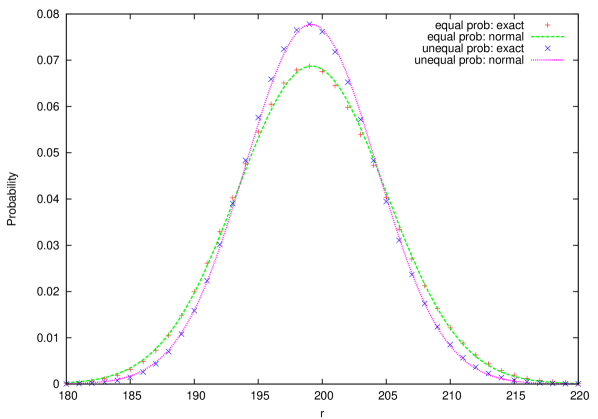
Figure 1: Distributions of positive signals when flow cycles $f=100$, for both equal and unequal nucleotide probabilities. The unequal nucleotide probabilities used here are $p_{a}=1/3=0.333$, $p_{b}=1/11=0.091$, $p_{c}=100/231=0.433$, and $p_{d}=1/7=0.143$. The exact distributions are calculated from Eqs. (16) and (2.2). The continuous curves are the normal distributions $N({\bar{r}}(f),\sigma_{r}^{2}(f))$ of the same mean and variance as those of the exact distributions, where ${\bar{r}}(f)$ and $\sigma_{r}^{2}(f)$ are calculated from Eqs. (17a) and (17b). The two normal distributions shown here are $N(199.167,33.681)$ and $N(199.130,26.316)$, for equal and unequal nucleotide probabilities, respectively.

2.6 Distribution of the number of flow cycles as a function of number of positive signals

To be complete, we derive here the distribution of the number of flow cycles $f$ at fixed number of positive signals $r$. The exact probability is expressed as

$$\frac{[x^{f}y^{r}]G(x,y)}{[y^{r}]G(1,y)}.$$ (18)

By using Eqs. (12) and (13) the mean and variance of $f$ at the fixed $r$ can be calculated as

$$\bar{f}(r) =\frac{1}{2}r+\frac{1}{2},$$ (19a)

$$\sigma^{2}_{f}(r) \approx\frac{e_{3}}{4e_{2}}r+\frac{2e_{2}^{3}+3e_{3}^{2}-2e_{2}e_{3}-4e_{2}e_{4}}{4e_{2}^{2}}.$$ (19b)

It should pointed out that Eq. (19a) is exact, while for Eq. (19b), only the dominant term corresponding to $y=1$ is kept while non-dominant terms are ignored.

It is interesting to note that like the mean of $r$, the mean of $f$ does not depend on the nucleotide probabilities. Again both the mean and variance vary linearly with the the number of positive signals $r$, as predicted by the singularity perturbation theory (Flajolet and Sedgewick, 2009). When the nucleotide probabilities are equal ($p_{i}=1/4$), the variance in Eq. (19b) becomes

$$\sigma^{2}_{f}(r)\approx\frac{1}{24}r+\frac{11}{96}.$$ (20)

In this equal nucleotide probability case the exact expression of $\sigma^{2}_{f}(r)$ can be written as

$$\sigma^{2}_{f}(r)=\frac{1}{24}r+\frac{11}{96}+\frac{15}{32}\left(-\frac{1}{3}\right)^{r},$$

with $15/32\times(-1/3)^{r}$ approaching zero as $r$ becomes large.

Based on the singularity perturbation theory (Flajolet and Sedgewick, 2009), the limiting distribution is again Gaussian. In Figure 2 the distributions of flow cycles when $r=200$ are plotted for both equal and unequal nucleotide probabilities. The unequal nucleotide probabilities used here are the same as in Figure 1. The exact distributions are calculated from Eqs. (18) and (2.2). Also shown in Figure 2 in continuous curves are the normal distributions $N({\bar{f}}(r),\sigma_{f}^{2}(r))$ of the same mean and variance as those of the exact distributions, where ${\bar{f}}(r)$ and $\sigma_{f}^{2}(r)$ are calculated from Eqs. (19a) and (19b). The two normal distributions shown here are $N(100.5,8.448)$ and $N(100.5,6.603)$, for equal and unequal nucleotide probabilities, respectively. As we can see from Figure 2, the exact distributions can be approximated accurately by the normal distributions with the same mean and variance, for both equal and unequal nucleotide probabilities.

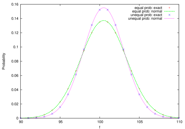
Figure 2: Distributions of the number of flow cycles when the number of positive signals $r=200$, for both equal and unequal nucleotide probabilities. The unequal nucleotide probabilities used here are the same as in Figure 1. The exact distributions are calculated from Eqs. (18) and (2.2). The continuous curves are the normal distributions $N({\bar{f}}(r),\sigma_{f}^{2}(r))$ of the same mean and variance as those of the exact distributions, where ${\bar{f}}(r)$ and $\sigma_{f}^{2}(r)$ are calculated from Eqs. (19a) and (19b). The two normal distributions shown here are $N(100.5,8.448)$ and $N(100.5,6.603)$, for equal and unequal nucleotide probabilities, respectively.

3 Fixed flow cycle model (FFCM)

In this model, instead of fixing the r-seq length $r$, we fix the number of flow cycles $f$. This is a more natural model than FRLM. As before (Kong, 2012), we assume that the sequence is generated by a random process that can create sequences with infinite length, only the first part of which will be sequenced by $f$ flow cycles. Let $P_{i}(f,r)$ ($i=a,b,c,d$) denote the probability that $f$ flow cycles will synthesize a sequence whose r-seq is of length $r$ and with the last incorporated nucleotide being $i$, and $P(f,r)$ be the sum of $P_{i}(f,r)$: $P(f,r)=\sum_{i\in\{a,b,c,d\}}P_{i}(f,r)$. Let $\mathcal{G}_{i}(x,y)$ be the GF of $P_{i}(f,r)$:

$$\mathcal{G}_{i}(x,y)=\sum_{r=1}^{\infty}\sum_{f=1}^{\infty}P_{i}(f,r)x^{f}y^{r}$$

and $\mathcal{G}(x,y)$ GF of $P(f,r)$: $\mathcal{G}(x,y)=\sum_{i\in\{a,b,c,d\}}\mathcal{G}_{i}(x,y)$. Using the same argument as before (Kong, 2012), we have the following relation between $P_{i}(f,r)$ and $L_{i}(f,r)$:

$$\begin{aligned} P_{a}(f,r)&=0,\\ P_{b}(f,r)&=L_{b}(f,r)p_{a},\\ P_{c}(f,r)&=L_{c}(f,r)(p_{a}+p_{b}),\ \\ P_{d}(f,r)&=L_{d}(f,r)(p_{a}+p_{b}+p_{c}).\end{aligned}$$ (21)

The first part of Eq. (21) is true because the first $f$ flow cycles can never synthesize a r-seq ending with $a$ and of length $r$. Based on our sequence model with the assumptions of complete nucleotide incorporation and infinite sequence length, if the next nucleotides to be synthesized are of type $a$, then they will be kept synthesized continuously within the nucleotide flow $a$ of flow cycle $f$ until a nucleotide that is not of type $a$ (say, a nucleotide of type $b$) comes up. Then this nucleotide will be synthesized within the nucleotide flow $b$ (if it is of type $b$) of flow cycle $f$, making the length of the r-seq $r+1$. The second part of Eq. (21) is true because if the first $f$ flow cycles are to synthesize a r-seq of length $r$ and ending with $b$, then the first $r$ positive signals of the sequence must be synthesized in the first $f$ flow cycles (which happens with probability proportional to $L_{b}(f,r)$), and no more positive signal must be synthesized in the $f$-th flow cycle. Only when the next base to be synthesized is of type $a$ can the synthesis in flow cycle $f$ be stopped; otherwise the synthesis will continue at the nucleotide flow $b$ if the next base is $b$, or the number of positive signals becomes $r+1$ if the next base is $c$ or $d$. The last two parts of Eq. (21) are true for similar reasons.

From Eq. (21) we can obtain similar relations between GFs $\mathcal{G}_{i}(x,y)$ and $G_{i}(x,y)$:

$$\begin{aligned} \mathcal{G}_{a}(x,y)&=0,\\ \mathcal{G}_{b}(x,y)&=G_{b}(x,y)p_{a},\\ \mathcal{G}_{c}(x,y)&=G_{c}(x,y)(p_{a}+p_{b}),\\ \mathcal{G}_{d}(x,y)&=G_{d}(x,y)(p_{a}+p_{b}+p_{c}).\end{aligned}$$ (22)

The GF $\mathcal{G}(x,y)=\sum_{i\in\{a,b,c,d\}}\mathcal{G}_{i}(x,y)$ thus calculated using Eq. (7) and above relations gives the distribution of $r$ for FFCM. It’s explicit form, however, is not as compact as Eq. (2.2) for FRLM so is not shown here. On the other hand, $\mathcal{G}(x,y)$ shows a nice property that Eq. (2.2) does not have:

$$\mathcal{G}(x,1)=\frac{x}{1-x}=x+x^{2}+x^{3}+\cdots,$$

which shows that $P(f,r)$ generated by $\mathcal{G}(x,y)$ is a probability distribution without the need for normalization as in FRLM in the previous sections: for any $f$, $\sum_{r=1}^{\infty}P(f,r)=1$.

From $\mathcal{G}(x,y)$ the mean and variance can be calculated as

$$\bar{r}(f) \approx 2f+\frac{e_{3}-e_{2}+p_{a}e_{2}+w}{e_{2}},$$ (23a)

$$\sigma^{2}_{r}(f) \approx\frac{2e_{3}}{e_{2}}f+\frac{3e_{3}^{2}-e_{2}e_{3}-2e_{2}e_{4}+p_{a}(1-p_{a})e_{2}^{2}-w^{2}+(2p_{b}p_{d}p_{c}^{2}+w)e_{2}}{e_{2}^{2}}$$ (23b)

where

$$w=p_{b}p_{c}p_{d}+p_{c}p_{b}^{2}+p_{d}p_{b}^{2}+p_{d}p_{c}^{2}.$$

We note that the mean and variance for FFCM (Eq. (23)) have the same coefficients of $f$ as in FRLM (Eq. (17)). They only differ in the constant terms. For FFCM, the constant terms are no longer symmetric for nucleotide probability $p_{i}$. For the special case of equal nucleotide probabilities, we have

$$\bar{r}(f) \approx 2f-\frac{5}{12},$$

$$\sigma^{2}_{r}(f) \approx\frac{1}{3}f+\frac{35}{144}.$$

Since $\mathcal{G}_{i}(x,y)$’s are linear transform of $G_{i}(x,y)$’s, $\mathcal{G}(x,y)$ is still a bivariate GF that obeys the singularity perturbation theory (Flajolet and Sedgewick, 2009). The limiting distribution of $P(f,r)$ is Gaussian and its mean and variance are linear function of $f$, as Eq. (23) shows.

4 Simulation

To check the analytical results of FFCM developed in this paper, we developed a simulation program written in C programming language. The program can be found in http://graphics.med.yale.edu/sbs/. All the results of this paper have been carefully checked against simulation results. Using seed $s=12345$ and repetition of $2\times 10^{7}$, for $f=100$, $p_{a}=0.333333333$, $p_{b}=0.090909091$, $p_{c}=0.432900433$, $p_{d}=0.142857143$, the simulation gives the mean and variance as $199.574162$ and $26.209019$ respectively. The theoretical results from Eq. (23) gives $199.573625$ and $26.215222$ for FFCM, which are closer to the simulation results than FRLM, which gives $199.129853$ and $26.315978$ as mean and variance (Eq. (17)). This simulation results are posted in the same website as the simulation program itself.

5 Some remarks on relations between $f$, $n$, and $r$

In this paper we have derived the relation between $f$, the number of flow cycles, and $r$, the number of positive signals in pyrograms. Previously, we have obtained the relation between $f$ and $n$, the sequence length (Kong, 2009a, 2012). The distribution of the number of runs $r$ in random sequences with a fixed length $n$ has also been derived (Kong, 2013). Here we summarize these relations below. The mean and variance of $n$ when $f$ is fixed for FFCM  (Kong, 2012)

$$\begin{aligned} \bar{n}(f)&\approx\frac{f}{e_{2}}+\frac{e_{3}}{e_{2}^{2}}-1,\\ \sigma^{2}(f)&\approx\frac{e_{2}+2e_{3}-3e_{2}^{2}}{e_{2}^{3}}f-\frac{e_{2}^{2}e_{3}-5e_{3}^{2}+4e_{2}e_{4}}{e_{2}^{4}}.\end{aligned}$$ (24)

The mean and variance of $r$ when $f$ is fixed for FFCM derived in this work are given by Eq. (23). The mean and variance of $r$ for a random sequence with a length of $n$ are given by  (Kong, 2013)

$$\bar{r}(n) =(1-P_{2})n+P_{2}$$

$$=2e_{2}n+1-2e_{2},$$ (25)

$$\sigma_{r}^{2}(n) =(P_{2}+2P_{3}-3P_{2}^{2})n-(P_{2}+4P_{3}-5P_{2}^{2})$$

$$=(4e_{2}+6e_{3}-12e_{2}^{2})n-(6e_{2}+12e_{3}-20e_{2}^{2}),$$ (26)

where $P_{j}=\sum_{i\in\{a,b,c,d\}}p_{i}^{j}$.

The average of these three distributions are transitive, if we ignore the small constant terms. If we use Eq. (24) to calculate the average of sequence length $n$ as a function of $f$, we have $\bar{n}(f)\approx f/e_{2}$. If we put it in Eq. (25) $\bar{r}(n)\approx 2e_{2}n$, we obtain $\bar{r}(f)\approx 2f$, which is correct based on the results from this work (Eq. (23a). For the variances, however, these transitive relations do not hold. For example, for equal probabilities $p_{i}=1/4$, the means and variances for the three distributions are summarized below. The first two equations are from FFCM.

$${\bar{n}}(f) \approx\frac{8}{3}f-\frac{5}{9} \sigma_{n}^{2}(f) \approx\frac{40}{27}f+\frac{20}{81},$$ (27)

$$\bar{r}(f) \approx 2f-\frac{5}{12} \sigma^{2}_{r}(f) \approx\frac{1}{3}f+\frac{35}{144}$$ (28)

$$\bar{r}(n) =\frac{3}{4}n+\frac{1}{4}, \sigma_{r}^{2}(n) =\frac{3}{16}n-\frac{3}{16}.$$ (29)

If we use Eq. (27) to get the average of sequence length ${\bar{n}}(f)\approx 8f/3$ and put it into Eq. (29), we end up with $\sigma_{r}^{2}(f)\approx f/2$, which is different from the correct expression shown in Eq. (28) as $\sigma_{r}^{2}(f)\approx f/3$. In fact, the variance $\sigma_{r}^{2}(f)$ will always be overestimated if we use Eq. (24) to get the average of sequence length $n$ as $\bar{n}(f)\approx f/e_{2}$ and use it in Eq. (26) to estimate $\sigma_{r}^{2}(f)$ as $\sigma_{r}^{2}(f)\approx(4e_{2}+6e_{3}-12e_{2}^{2})f/e_{2}$. By using the constrain $e_{1}=1$, it can be shown that $(4e_{2}+6e_{3}-12e_{2}^{2})/e_{2}$ is always more than $3/2$ times bigger than $2e_{3}/e_{2}$, the correct coefficient of $f$ for $\sigma^{2}_{r}(f)$, as shown in Eq.(23b) or Eq.(17b).

References

- Balakrishnan and Koutras (2002) Balakrishnan N, Koutras MV (2002) Runs and Scans with Applications. John Wiley & Sons, New York
- Flajolet and Sedgewick (2009) Flajolet P, Sedgewick R (2009) Analytic Combinatorics. Cambridge University Press, New York, NY, USA
- Kong (2006) Kong Y (2006) Distribution of runs and longest runs: A new generating function approach. Journal of the American Statistical Association 101:1253–1263
- Kong (2009a) Kong Y (2009a) Statistical distributions of pyrosequencing. J Comput Biol 16:31–42, DOI 10.1089/cmb.2008.0106
- Kong (2009b) Kong Y (2009b) Statistical distributions of sequencing by synthesis with probabilistic nucleotide incorporation. J Comput Biol 16:817–827, DOI 10.1089/cmb.2008.0215
- Kong (2012) Kong Y (2012) Length distribution of sequencing by synthesis: fixed flow cycle model. J Math Biol DOI 10.1007/s00285-012-0556-3
- Kong (2013) Kong Y (2013) Distributions of runs revisited. Communications in Statistics - Theory and Methods To appear