Length distribution of sequencing by synthesis: fixed flow cycle model

Abstract

Sequencing by synthesis is the underlying technology for many next-generation DNA sequencing platforms. We developed a new model, the fixed flow cycle model, to derive the distributions of sequence length for a given number of flow cycles under the general conditions where the nucleotide incorporation is probabilistic and may be incomplete, as in some single-molecule sequencing technologies. Unlike the previous model, the new model yields the probability distribution for the sequence length. Explicit closed form formulas are derived for the mean and variance of the distribution.

1 Introduction

The next-generation sequencing (NGS) technology has transformed biology and biomedical research by generating huge amount of sequence data at unprecedented speed. The emerging DNA sequencing technology also gave rise to many interesting mathematical and statistical problems. One of these problems is the statistical distributions of various quantities associated with sequencing by synthesis (SBS) technology. Besides its practical applications in different stages in the development and use of NGS technology, such as instrument development and testing, algorithm and software development, as well as daily monitoring of sequencing outputs, the problem is an interesting self-contained mathematical problem.

Unlike the traditional Sanger capillary electrophoresis method using dideoxynucleotide chain-termination, many of the currently available platforms and those that are still under development utilize SBS technology. In SBS platforms, nucleotides are added to the reactions repeatedly in a pre-determined cyclic manner. In a particular nucleotide cycle, if the added nucleotide is complementary to the base in the template (the DNA to be sequenced), then the nucleotide will be potentially synthesized by the enzyme (DNA polymerase) and a signal can be detected. Since we know what nucleotide is added in that cycle, the base in the template can be determined. If the dispensed nucleotide is not complementary to the base in the template, or due to the probabilistic nature of the enzymatic synthesis reaction (see subsection 1.1.2 below), the nucleotide will not be incorporated in this nucleotide cycle. Apparently, the length of sequence that can be read from the DNA template is not a linear function of the number of nucleotide cycles but rather depends on the sequence context, the nucleotide flow order, and the reaction conditions that determine the nucleotide incorporation probabilities.

We have studied the sequence length distributions of SBS previously (Kong, 2009a, b). There the problem was approached indirectly. In that model (see subsection 1.2.1 below) we fixed the sequence length and the probability distribution obtained is actually the distribution of flow cycle for a given sequence length. It would be more interesting to obtain directly the distribution of sequence length for a given flow cycle. In the previous work we did obtain the sequence length distribution, but that had to be done by using some approximate normalization. In this paper we developed a new model, the fixed sequence length model (FSLM), from which we obtain directly the sequence length distribution at a given flow cycle. This model is more natural than the previous model as it allows for exact computation of the associated probability distribution, while the previous model only yielded approximations. Furthermore, the new model will be the basis on which other statistical quantities of SBS platforms will be investigated in future studies.

In subsection 1.2 the old and new models are to be discussed. Before that, some basics of SBS technology will first be introduced. After this introduction section, the complete and incomplete nucleotide incorporation cases will be studied in section 2 and section 3 respectively. The main results are Eqs. (19), (20), and (21) for the general incomplete nucleotide incorporation conditions, with Eqs. (7), (9) and (10) as their special cases for complete nucleotide incorporation conditions.

1.1 SBS technology

As mentioned earlier, SBS technology adds four nucleotides $A$, $C$, $G$, and $T$ repeatedly in a pre-determined order. To avoid the unnecessary specification of the detailed names of the four kinds of nucleotides, in the following we will use $a$, $b$, $c$, and $d$ to represent any permutations of the usual nucleotides $A$, $C$, $G$, and $T$, as we did previously.

We call each of the four cycles where nucleotides are added a nucleotide cycle. A flow cycle is defined as the “quad cycle” of successive four nucleotides cycles of {$abcd$}, with “$a$” the first nucleotide in the flow cycle and “$d$” the last nucleotide in the same flow cycle.

SBS reads the template DNA by synthesizing the base that is complementary to the current base to be read in the template DNA. Nucleotide $A$ is complementary to $T$, and $C$ to $G$. After the complementary nucleotide is incorporated, certain kind of signal can be detected, usually through fluorescence dye attached to the incorporated nucleotide. The detected signal is registered with the pre-determined nucleotide cycle, so the nature of the incorporated nucleotide can be determined. Ideally, if we ignore noises and errors, and if the added nucleotide is not complementary to the base in the template DNA, then in that nucleotide cycle no signal will be created. If the added nucleotide is complementary to the template, however, we have two possibilities, depending on what kind of NGS technology we are dealing with. In the following we discuss two variations of SBS technologies, bulk sequencing and single-molecule sequencing, and the different degree of completeness of nucleotide incorporation associated with the two technologies.

1.1.1 Bulk SBS and complete nucleotide incorporation

For bulk SBS sequencing technologies such as pyrosequencing, the template DNAs go through a clonal amplification step before sequencing. What gets sequenced is actually a collection of identical template molecules. During the sequencing process, the synchronization between identical individual templates will be lost gradually, leading to signal decay and sequencing errors. To avoid this dephasing problem, the reaction reagents and synthesis chemistry are usually tuned to drive the enzymatic incorporation to completion at each nucleotide cycle. Not only will a single base, if it is complementary to the template base, be incorporated, but also a stretch of identical bases (homopolymers) will be synthesized in the same nucleotide cycle. For example, if the template DNA has three $G$’s together, then in one nucleotide cycle of $C$ three nucleotides of $C$ will be incorporated to match each $G$ in the template. In ideal conditions for complete nucleotide incorporation, the sequence context and nucleotide flow order uniquely determine the emitted signals.

For example, for sequence bddabaaad, with complete nucleotide incorporation the signal will be {0-1-0-2}-{1-1-0-0}-{3-0-0-1}, while for another sequence abbbdabbc with the same length, the signal will be {1-3-0-1}-{1-2-1-0}, if we assume that the strength of the signal is proportional to the number of nucleotides incorporated in each nucleotide cycle (Table 1, Kong (2009a)). Here we use the four numbers within the braces to indicate the signal strength of each nucleotide cycle within a flow cycle. For example, the number $3$ in the signal for the second sequence (the second nucleotide cycle in the first flow cycle) corresponds to the three consecutive $b$’s in the second sequence.

1.1.2 Single-molecule SBS and incomplete nucleotide incorporation

Some NGS platforms that have been commercially available recently or are under active development utilize single-molecule DNA sequencing (SMS) technology. Unlike the bulk sequencing platforms, SMS does not have a clonal amplification step for the target sequences. Instead, a single target molecule is used as the template. This avoids the problems of bias and errors introduced in the amplification step. Another advantage of SMS is that the problem of dephasing associated with bulk sequencing methods mentioned above does not exist for SMS. For this reason, the reaction kinetics can be controlled to adjust the rate of nucleotide incorporation to the benefit of sequencing accuracy. For example, slow reaction kinetics can be used deliberately to limit incorporation to two or three bases per nucleotide cycle (Harris et al, 2008). For a homopolymer region GGG, bulk sequencing technology will try to incorporate three $C$’s in one nucleotide cycle; for SMS, however, zero, one, two, or three $C$’s can be incorporated in a single synthesis cycle. This flexibility in incorporation rate can be utilized to increase the resolution of homopolymer region. Under these conditions, even if the dispensed nucleotide for a given cycle is complement to the base in the template, the nucleotide might not be incorporated in the current nucleotide cycle. The incorporation of the nucleotide may be delayed to the next cycle, or the next next cycle, and so on. Which cycle the nucleotide will be incorporated will depend probabilistically on the reaction conditions. Thus, the signal will not be deterministically determined by the sequence context and flow order alone; in addition it will also depend on the nucleotide incorporation probability. Under incomplete nucleotide incorporation conditions, the same template sequence will potentially generate many different signals. This kind of combinatorial explosion makes the question of studying the sequence length distribution more complicated than under the complete nucleotide incorporation conditions. There are, however, mathematics tools that can solve the problem nicely, and the solutions to both complete incorporation and incomplete incorporation are united, with the former being a special case of the latter.

1.2 Fixed sequence length model and fixed flow cycle model

1.2.1 Fixed sequence length model (FSLM)

Two models can be used to investigate various statistic distributions of SBS. One model, which was used in our previous work, can be termed as fixed sequence length model (FSLM). In this model the length of the template DNA sequences is pre-defined as $n$. Thus, with $4$ possible bases at each position, the total number of sequences for a given $n$ is $4^{n}$.

For FSLM with a given sequence length $n$, the minimum number of nucleotide flows is $1$, for a stretch of $n$ $a$’s. The maximum number of nucleotide flows under complete nucleotide incorporation conditions is $3n+1$, for sequence dcbadcba.... In this case the maximum flow cycle is $f=\lceil(3n+1)/4\rceil$. Thus for a fixed sequence length $n$, the range of flow cycle $f$ is $[1,\lceil(3n+1)/4\rceil]$. For incomplete nucleotide incorporation conditions, the upper limit of the range is determined by the nucleotide incorporation probabilities.

Within this model, we have derived the generating function (GF) for $L_{i}(n,f)$, the probability that a sequence of length $n$ and ending with nucleotide $i$, $i=a,b,c,d$, is synthesized in the first $f$ flow cycles, with the $n$-th nucleotide being synthesized in flow cycle $f$. With the assumption that the nucleotides in the target sequence are independent random variables with probabilities $p_{a},p_{b},p_{c}$, and $p_{d}$, and under complete nucleotide incorporation conditions, the first few values of $L_{i}(n,f)$ are shown in Table 1. Here and in the following the tables are arranged so that each row is for a given sequence length $n$, and every four columns are for a given flow cycle $f$, with each of the four columns within a given flow cycle $f$ corresponding to the nucleotide synthesized, in the order of $a$, $b$, $c$, $d$. As we have shown, each row in Table 1 sums to $1$,

$$\sum_{f=1}^{\infty}\sum_{i\in\{a,b,c,d\}}L_{i}(n,f)=1,$$

so for FSLM, $L_{i}(n,f)$ is the probability over the flow cycle $f$ for a fixed sequence length $n$.

Table 1: The first few values of $L_{i}(n,f)$ for fixed sequence length model (FSLM) for complete nucleotide incorporation case. This model is used previously but not in this paper. The recursive structure of $L_{i}(n,f)$ is readily evident. Here $L_{d}(2,1)=(p_{a}+p_{b}+p_{c}+p_{d})p_{d}=p_{d}$. For each row, the sum of $L_{i}(n,f)$ is $1$: $\sum_{f=1}^{\infty}\sum_{i\in\{a,b,c,d\}}L_{i}(n,f)=1$.

	$f=1$				$f=2$
$n$	$a$	$b$	$c$	$d$	$a$	$b$	$c$	$d$
$1$	$p_{a}$	$p_{b}$	$p_{c}$	$p_{d}$	$0$	$0$	$0$	$0$
$2$	$p_{a}^{2}$	$(p_{a}+p_{b})p_{b}$	$(p_{a}+p_{b}+p_{c})p_{c}$	$p_{d}$	$(p_{b}+p_{c}+p_{d})p_{a}$	$(p_{c}+p_{d})p_{b}$	$p_{d}p_{c}$	0

The value of $L_{i}(n,f)$ gives the probability that for a given sequence length $n$ , the sequence can be sequenced in $f$ flow cycles with the last base as $i$. The more interesting question, the answer to which will have more practical uses, is the distribution of sequence length for a given flow cycle $f$. To get the answer to this question we have to look at the columns in Table 1 instead of rows. The sum of the entries for each column (fixed $f$) in Table 1, or every four columns within each $f$, however, does not add up to $1$, so we have to normalize the entries to transform them into probabilities. For FSLM, only approximate closed form normalization factors can be found, though the errors of the approximation are small and become negligible when $f$ becomes bigger.

This somewhat unsatisfactory detour motivated us to develop a model that directly yields the distribution of sequence length for a fixed number $f$ of flow cycles. The model, fixed flow cycle model (FFCM), is the main focus of this paper.

1.2.2 Fixed flow cycle model (FFCM)

In this model, instead of fixing the sequence length, we fix the number of flow cycles. We assume that the sequence is generated by a random process that can create sequences with infinite length, only the first part of which will be sequenced by $f$ flow cycles. In other words, for a fixed number $f$ of flow cycles, we assume that the target sequence is always longer than that can be sequenced by $f$ cycles. We also assume that the flow cycle $f$ is always a complete cycle (i.e., the number of nucleotide cycles is always a multiple of $4$). With FFCM, the size of sample space becomes infinite. For example, for $f=1$, the sequence ba... can only get the first base b sequenced, while the hypothetical sequence bbbbbb... can in theory get infinite read length for the first cycle. Hence for $f=1$, in the first case the sequence length $n=1$, while for the second case the sequence length $n\rightarrow\infty$. We’re interested in the probability distribution of the sequence length $n$ for a given $f$.

1.3 Simulations

For FSLM, there are a finite number of sequences ($4^{n}$ for sequence length $n$). Under complete nucleotide incorporation conditions, the range of flow cycle is also finite (see subsection 1.2.1), so the sample space is finite. The analytical results can be checked by enumeration over all possible points in this space. Indeed, all results previously obtained for FSLM have been checked by enumerations. For FFCM, however, the sample space is infinite, and we cannot enumerate all possible configurations in its sample space. To check the analytical results of FFCM developed in this paper, we developed a simulation program written in C programming language. The program can be found in http://graphics.med.yale.edu/sbs/. All the results of this paper have been carefully checked against simulation results.

1.4 Notation and Definitions

As mentioned above, we use $a$, $b$, $c$, and $d$ to represent any permutations of the usual nucleotides $A$, $C$, $G$, and $T$ to avoid the unnecessary specification of the detailed names of the four kinds of nucleotides. The probabilities for the four nucleotides in the target sequence are denoted as $p_{a}$, $p_{b}$, $p_{c}$, and $p_{d}$, with $\sum_{i\in\{a,b,c,d\}}p_{i}=1$. We assume that the nucleotides in the target sequence are independent of each other. We always use $f$ for the number of flow cycles, and $n$ as the length of sequenced reads. To avoid extra symbols, we often use the bases themselves when their complements should be used, if no ambiguity arises. For example, if the base in the template to be sequenced is $b$, then it’s the complement of $b$ that can be added chemically, but we will still use $b$ instead of the complement of $b$ in the following developments.

The nucleotide incorporation probabilities are denoted as $\alpha_{j}^{(i)}$, where $i=a$, $b$, $c$, and $d$ stands for the type of nucleotides, $j=0$, $1$, $2$, $\dots$ denotes the delayed flow cycle number, with the current flow cycle as $0$. The value of $\alpha_{j}^{(i)}$ is the probability that the next nucleotide of type $i$ will be incorporated in the $j$-th cycle from the current flow cycle. For example, when it is complementary to the template, if the chance for nucleotide $b$ to be incorporated in the current cycle, the next cycle, and the next-next cycle is $1/3$, $1/2$, and $1/6$, respectively, then $\alpha_{0}^{(b)}=1/3$, $\alpha_{1}^{(b)}=1/2$, $\alpha_{2}^{(b)}=1/6$, and $\alpha_{j}^{(b)}=0$ for $j>2$. The complete incorporation situation is a special case in this notation with $\alpha_{0}^{(i)}=1$ and $\alpha_{j}^{(i)}=0$ for $j>0$. By definition $\sum_{j=0}^{\infty}\alpha_{j}^{(i)}=1$. The GFs of $p_{i}\alpha_{j}^{(i)}$ is denoted by $g_{i}(x)$ ($i=a$, $b$, $c$, and $d$):

$$g_{i}(x)=p_{i}\sum_{j=0}^{\infty}\alpha_{j}^{(i)}x^{j}.$$ (1)

We note that when $x=1$, $g_{i}(1)=p_{i}$. Also, for the complete incorporation situation, $g_{i}(x)=p_{i}$.

To extract coefficients from expansion of GFs, we use notation $[x^{n}]f(x)$ to denote the coefficient of $x^{n}$ in the series of $f(x)$ in powers of $x$.

In Table 2 the common notation used throughout the paper is summarized in one place. Some of the detailed definitions will be deferred to the relevant sections in the following.

Table 2: Summary of notation and definitions.

	Definition	Comments
$f$	flow cycle	$f=1,2,\dots$
$n$	sequence length	$n=0,1,\dots$
$a$, $b$, $c$, $d$	any permutation of the 4 nucleotides
$p_{i}$	nucleotide probability	$i=a,b,c,d$
$\alpha_{j}^{(i)}$	nucleotide incorporation probability of nucleotide type $i$ that the next nucleotide will be incorporated in the $j$-th cycle from the current cycle	$i=a,b,c,d$, $j=0,1,\dots$; $\sum_{j=0}^{\infty}\alpha_{j}^{(i)}=1$
$\omega_{i}$	conditional factors of nucleotide type $i$, for complete nucleotide incorporation	$i=a,b,c,d$
$\omega_{j}^{(i)}$	conditional factors of nucleotide type $i$, for incomplete nucleotide incorporation	$i=a,b,c,d$, $j=0,1,\dots$
$P_{i}(n,f)$	probability that $f$ flow cycles will synthesize a sequence of length of $n$ and with the last incorporated nucleotide being $i$	$i=a,b,c,d$
$P(n,f)$	sum of $P_{i}(n,f)$	$P(n,f)=\sum_{i\in\{a,b,c,d\}}P_{i}(n,f)$
$L_{i}(n,f)$	probability that a sequence of length $n$ and ending with nucleotide $i$ is synthesized in the first $f$ flow cycles, with the $n$-th nucleotide being synthesized in flow cycle $f$	$i=a,b,c,d$
$L(n,f)$	sum of $L_{i}(n,f)$	$L(n,f)=\sum_{i\in\{a,b,c,d\}}L_{i}(n,f)$
$g_{i}(x)$	GF of $p_{i}\alpha_{j}^{(i)}$	$g_{i}(x)=p_{i}\sum_{j=0}^{\infty}\alpha_{j}^{(i)}x^{j}$
$h_{i}(x)$	GF of $\omega_{j}^{(i)}$	$h_{i}(x)=\sum_{j=0}^{\infty}\omega_{j}^{(i)}x^{j}$
$\mathcal{G}_{i}(x)$	GF of $P_{i}(n,f)$	$\mathcal{G}_{i}(x,y)=\sum_{n=0}^{\infty}\sum_{f=1}^{\infty}P_{i}(n,f)x^{f}y^{n}$
$\mathcal{G}(x)$	sum of $\mathcal{G}_{i}(x)$	$\mathcal{G}(x)=\sum_{i\in\{a,b,c,d\}}\mathcal{G}_{i}(x)$
$G_{i}(x)$	GF of $L_{i}(n,f)$	$G_{i}(x,y)=\sum_{n=0}^{\infty}\sum_{f=1}^{\infty}L_{i}(n,f)x^{f}y^{n}$
$G(x)$	sum of $G_{i}(x)$	$G(x)=\sum_{i\in\{a,b,c,d\}}G_{i}(x)$
$e_{i}$	elementary symmetric functions of $p_{i}$	$i=1,\cdots,4$, Eq. (6)
$t_{i}(x)$	elementary symmetric functions of $g_{i}(x)$	$i=1,\cdots,4$, Eq. (18)

2 Complete nucleotide incorporation

In this section the complete nucleotide incorporation conditions will be studied. As we showed previously, the key to the solution of FSLM is the set of recursive equations of $L_{i}(n,f)$. The set of equations cannot be solved analytically, but transforming them into GFs leads to exact solutions of these GFs. The recursive structure is evident in the elements in Table 1.

For FFCM, let $P_{i}(n,f)$ denote the probability that $f$ flow cycles will synthesize a sequence of length of $n$ and with the last incorporated nucleotide being $i$, and let $P(n,f)=\sum_{i\in\{a,b,c,d\}}P_{i}(n,f)$ be the probability that in $f$ flow cycles the sequenced length is $n$. For this section only, with complete nucleotide incorporation conditions, the sequence length $n$ starts from $1$, since in this case the probability $P(n,f)$ for $n=0$ is zero. For the incomplete nucleotide incorporation case discussed later in section 3, however, the probability to have $n=0$ is nonzero, and the case of $n=0$ will be considered there.

With this definition, it is evident that we have the following simple equations to link the probabilities $L_{i}(n,f)$ of FSLM and the probabilities $P_{i}(n,f)$ of FFCM:

$$P_{a}(n,f) =0,$$ (2)

$$P_{b}(n,f) =L_{b}(n,f)p_{a},$$

$$P_{c}(n,f) =L_{c}(n,f)(p_{a}+p_{b}),$$

$$P_{d}(n,f) =L_{d}(n,f)(p_{a}+p_{b}+p_{c}).$$

The first part of Eq. (2) is true because the first $f$ flow cycles can never synthesize a sequence ending with $a$ and of length $n$. Indeed, irrespective of the type of the $(n+1)$-st nucleotide, it will always be synthesized in the same flow cycle so the length cannot be $n$. The second part of Eq. (2) is true because if the first $f$ flow cycles are to synthesize a sequence of length $n$ and ending with $b$, then the first $n$ nucleotides of the sequence must be synthesized in the first $f$ flow cycles (which happens with probability $L_{b}(n,f)$), and then no more nucleotide must be synthesized in the $f$-th flow cycle (because otherwise the first $f$ flow cycles will synthesize more than $n$ nucleotides). The latter in turn implies that the $(n+1)$-st nucleotide of the sequence must be $a$, which happens with probability $p_{a}$. The last two parts of Eq. (2) are true for similar reasons.

The first few values of $P_{i}(n,f)$ are listed in Table 3. Note the factors $\omega_{i}$ in $P_{i}(n,f)$ of Table 3 when they’re compared with $L_{i}(n,f)$ of Table 1. The four conditional factors are

$$\omega_{a}=0,\quad\omega_{b}=p_{a},\quad\omega_{c}=p_{a}+p_{b},\quad\text{and}\quad\omega_{d}=p_{a}+p_{b}+p_{c}.$$ (3)

Table 3: The first few values of $P_{i}(n,f)$ for fixed flow cycle model (FFCM) under complete nucleotide incorporation conditions. Note the factors $\omega_{i}$ when compared with the entries $L_{i}(n,f)$ in Table 1. These factors are listed in Eq. (3). For each $f$, the sum of the four columns of $P_{i}(n,f)$ is $1$: $\sum_{n=0}^{\infty}\sum_{i\in\{a,b,c,d\}}P_{i}(n,f)=1$.

	$f=1$				$f=2$
$n$	$a$	$b$	$c$	$d$	$a$	$b$	$c$	$d$
$1$	$p_{a}\omega_{a}$	$p_{b}\omega_{b}$	$p_{c}\omega_{c}$	$p_{d}\omega_{d}$	$0$	$0$	$0$	$0$
$2$	$p_{a}^{2}\omega_{a}$	$(p_{a}+p_{b})p_{b}\omega_{b}$	$(p_{a}+p_{b}+p_{c})p_{c}\omega_{c}$	$p_{d}\omega_{d}$	$0$	$(p_{c}+p_{d})p_{b}\omega_{b}$	$p_{d}p_{c}\omega_{c}$	0
$\cdots$	$\cdots$	$\cdots$	$\cdots$	$\cdots$	$\cdots$	$\cdots$	$\cdots$	$\cdots$

The equations of probabilities $P_{i}(n,f)$ and $L_{i}(n,f)$ in Eq. (2) can then be transformed into relations between their GFs:

$$\mathcal{G}_{a}(x,y) =0,$$ (4)

$$\mathcal{G}_{b}(x,y) =G_{b}(x,y)p_{a},$$

$$\mathcal{G}_{c}(x,y) =G_{c}(x,y)(p_{a}+p_{b}),$$

$$\mathcal{G}_{d}(x,y) =G_{d}(x,y)(p_{a}+p_{b}+p_{c}),$$

where $\mathcal{G}_{i}(x,y)$ is the bivariate GF of $P_{i}(n,f)$:

$$\mathcal{G}_{i}(x,y)=\sum_{n=0}^{\infty}\sum_{f=1}^{\infty}P_{i}(n,f)x^{f}y^{n},\qquad i=a,b,c,d,$$

and $G_{i}(x,y)$ is the bivariate GF of $L_{i}(n,f)$:

$$G_{i}(x,y)=\sum_{n=0}^{\infty}\sum_{f=1}^{\infty}L_{i}(n,f)x^{f}y^{n},\qquad i=a,b,c,d.$$

Since $G_{i}(x,y)$’s have been solved previously (Eqs. (4)-(7), Kong (2009a)), $\mathcal{G}_{i}(x,y)$ can be easily obtained from Eq. (4):

$$\mathcal{G}_{a}(x,y) =0,$$ (5)

$$\mathcal{G}_{b}(x,y) =\frac{p_{a}p_{b}xy}{H}\left[1-(p_{c}+p_{d})(1-x)y+p_{c}p_{d}(1-x)^{2}y^{2}\right],$$

$$\mathcal{G}_{c}(x,y) =\frac{(p_{a}+p_{b})p_{c}xy}{H}\left[1-p_{d}(1-x)y\right],$$

$$\mathcal{G}_{d}(x,y) =\frac{(p_{a}+p_{b}+p_{c})p_{d}xy}{H},$$

where

$$H=1-y+e_{2}(1-x)y^{2}-e_{3}(1-x)^{2}y^{3}+e_{4}(1-x)^{3}y^{4}.$$

Here $e_{i}$’s are elementary symmetric functions (ESFs) of nucleotide probabilities $p_{i}$:

$$e_{1} =p_{a}+p_{b}+p_{c}+p_{d}=1,$$ (6)

$$e_{2} =p_{a}p_{b}+p_{a}p_{c}+p_{a}p_{d}+p_{b}p_{c}+p_{b}p_{d}+p_{c}p_{d},$$

$$e_{3} =p_{a}p_{b}p_{c}+p_{a}p_{b}p_{d}+p_{a}p_{c}p_{d}+p_{b}p_{c}p_{d},$$

$$e_{4} =p_{a}p_{b}p_{c}p_{d}.$$

We’re mainly interested in $P(n,f)$, the probability of read length as $n$ for a given flow cycle $f$. Since $P(n,f)$ is the sum of $P_{i}(n,f)$’s, the GF of $P(n,f)$, $\mathcal{G}(x,y)$, is the sum of $\mathcal{G}_{i}(x,y)$’s:

$$\mathcal{G}(x,y)=\sum_{i\in\{a,b,c,d\}}\mathcal{G}_{i}(x,y)=\frac{xy}{H}\left[e_{2}-e_{3}(1-x)y+e_{4}(1-x)^{2}y^{2}\right].$$ (7)

In comparison, the $G(x,y)$ of FSLM, which is the sum of $G_{i}(x,y)$’s, is given by

$$G(x,y)=\frac{xy}{H}[1-e_{2}(1-x)y+e_{3}(1-x)^{2}y^{2}-e_{4}(1-x)^{3}y^{3}].$$

Although $\mathcal{G}(x,y)$ and $G(x,y)$ look similar to each other, $G(x,y)$ is the probability generating function (pgf) for FSLM where sequence length $n$ is fixed, while $\mathcal{G}(x,y)$ is the pgf of FFCM where flow cycle $f$ is fixed. To check that $P(n,f)$ generated by GF in Eq. (7) is a probability distribution over $n$, we see that

$$\mathcal{G}(x,1)=\frac{x}{1-x}=x+x^{2}+x^{3}+\cdots,$$

so that $\sum_{n=1}^{\infty}P(n,f)=1$ for any $f$. On the other hand,

$$G(1,y)=\frac{y}{1-y}=y+y^{2}+y^{3}+\cdots,$$

so that $\sum_{f=1}^{\infty}L(n,f)=1$ for any $n$.

From Eq. (5) or Eq. (7) we can in principle calculate exactly $P_{i}(n,f)$ or $P(n,f)$ for any $f$ and $n$. In Figure 1 the distribution of sequence length are shown for the first $10$ flow cycles ($f=1,2,\dotsc,10$). The nucleotide composition probabilities used here are $p_{a}=1/3=0.3333$, $p_{b}=1/11=0.0909$, $p_{c}=100/231=0.4329$, and $p_{d}=1/7=0.1429$. The distribution is calculated from Eq. (7).

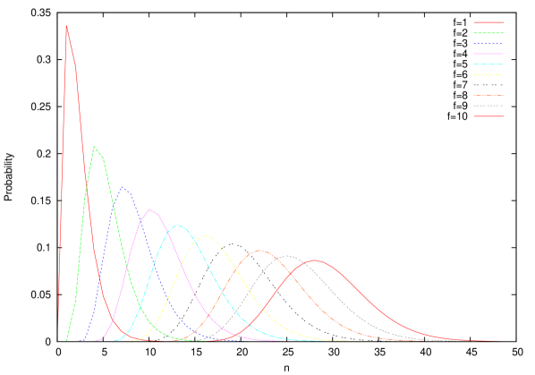
Figure 1: The distribution of sequence length for the first $10$ cycles ($f=1,2,\dotsc,10$) with complete nucleotide incorporation. The nucleotide composition probabilities used here are $p_{a}=1/3=0.3333$, $p_{b}=1/11=0.0909$, $p_{c}=100/231=0.4329$, and $p_{d}=1/7=0.1429$. The distribution is calculated from Eq. (7).

2.1 Mean and variance

From GF Eq. (7) the mean and variance of the sequence length distribution $P(n,f)$ at a given number of flow cycles $f$ can be calculated:

$$\bar{n}(f) =[x^{f}]\left.\frac{\partial\mathcal{G}(x,y)}{\partial y}\right|_{y=1},$$ (8a)

$$\sigma^{2}(f) =[x^{f}]\left.\frac{\partial^{2}\mathcal{G}(x,y)}{\partial y^{2}}\right|_{y=1}+\bar{n}(f)-\bar{n}^{2}(f).$$ (8b)

To get closed form formulas for $\bar{n}(f)$ and $\sigma^{2}(f)$, we note that $x=1$ is a singularity in both $\left.\partial\mathcal{G}(x,y)/\partial y\right|_{y=1}$ and $\left.\partial^{2}\mathcal{G}(x,y)/\partial y^{2}\right|_{y=1}$. The denominator of Eq. (8a) has a $(x-1)^{2}$ factor:

$$(x-1)^{2}(e_{2}-e_{3}+e_{4}+(e_{3}-2e_{4})x+e_{4}x^{2}),$$

and the denominator of Eq. (8b) has a $(x-1)^{3}$ factor:

$$(x-1)^{3}(e_{2}-e_{3}+e_{4}+(e_{3}-2e_{4})x+e_{4}x^{2})^{2}.$$

For both Eq. (8a) and Eq. (8b) $x=1$ is the pole that has the smallest module. By using only the principal part of the series expansion, we obtain the closed form formulas for $\bar{n}(f)$ and $\sigma^{2}(f)$ as

$$\bar{n}(f)\approx\frac{f}{e_{2}}+\frac{e_{3}}{e_{2}^{2}}-1,$$ (9)

and

$$\sigma^{2}(f)\approx\frac{e_{2}+2e_{3}-3e_{2}^{2}}{e_{2}^{3}}f-\frac{e_{2}^{2}e_{3}-5e_{3}^{2}+4e_{2}e_{4}}{e_{2}^{4}}.$$ (10)

When these formulas are compared with the corresponding closed form formulas of FSLM (Eq. (20) and Eq. (21), Kong (2009a)), we see that again both the mean and variance are linear functions of $f$. Furthermore, the coefficients of $f$ are the same in both models. The only differences are in the constant terms.

For the special case of equal base probability where $p_{a}=p_{b}=p_{c}=p_{d}=1/4$, we have

$$\bar{n}(f) \approx\frac{8}{3}f-\frac{5}{9},$$

$$\sigma^{2}(f) \approx\frac{40}{27}f+\frac{20}{81}.$$

In Table 4 the differences between the approximate and exact values of the mean (Eq. (9)) and the variance (Eq. (10)) are shown for the first few values of $f$, with the same parameters of nucleotide probabilities as those in Figure 1. The exact values are calculated from Eq. (8a) and Eq. (8b). As we can see, the approximations are very good: for flow cycle as small as $f=5$ the approximate and exact values are already very close.

Table 4: Comparisons of the closed form approximations and exact values of the mean (Eq. (9)) and the variance (Eq. (10)) for the first few values of $f$, with the same parameters as those in Figure 1. The exact values are calculated from Eq. (8a) and Eq. (8b).

	$\bar{n}(f)$		$\sigma^{2}(f)$
$f$	Eq. (9)	exact mean	Eq. (10)	exact variance
1	2.35859351	2.39446565	2.37546292	2.25930624
2	5.33118557	5.32877823	4.58883999	4.60388485
3	8.30377762	8.30387577	6.80221706	6.80137770
4	11.27636968	11.27637169	9.01559413	9.01555228
5	14.24896173	14.24896084	11.22897120	11.22898734
6	17.22155379	17.22155390	13.44234827	13.44234604
7	20.19414585	20.19414584	15.65572534	15.65572555
8	23.16673790	23.16673790	17.86910241	17.86910240
9	26.13932996	26.13932996	20.08247948	20.08247948
10	29.11192201	29.11192201	22.29585655	22.29585655

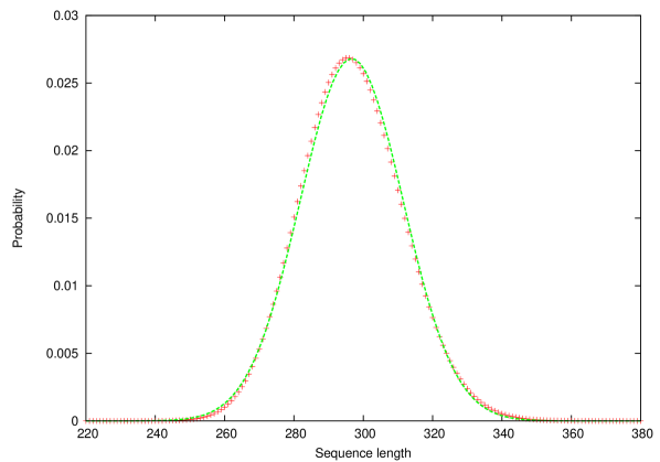
Figure 2: The distribution of sequence length with complete nucleotide incorporation for a fixed flow cycle of $f=100$. The nucleotide composition probabilities used here are the same as in Figure 1. The exact distribution is plotted as ’+’ and is calculated from Eq. (7). The continuous curve is the normal distribution $N({\bar{n}}(f),\sigma^{2}(f))$ of the same mean and variance as those of the exact distribution, where ${\bar{n}}(f)$ and $\sigma^{2}(f)$ are calculated from Eqs. (9) and (10). The normal distribution shown here is $N(296.6452,221.4998)$.

In Figure 2 the distribution of sequence length $P(n,f)$ with complete nucleotide incorporation for flow cycle $f=100$ is shown, together with a normal distribution with the same mean and variance. The nucleotide composition probabilities used here are the same as in Figure 1. The exact distribution is plotted as ’+’ and is calculated from Eq. (7). The continuous curve is the normal distribution $N({\bar{n}}(f),\sigma^{2}(f))$ of the same mean and variance as those of the exact distribution $P(n,f)$, where ${\bar{n}}(f)$ and $\sigma^{2}(f)$ are calculated from Eqs. (9) and (10). The normal distribution shown in Figure 2 is $N(296.6452,221.4998)$. As Figure 2 shows, the normal distribution fits the distribution of $P(n,f)$ quite well, with the exact distribution slightly skews to the left and has a slightly thick tail on the right. The approximate normality of the number of nucleotides synthesized over $f$ flow cycles is not surprising if we make a central limit theorem type of argument. This number is the sum of the number of nucleotides synthesized in each of the $f$ flow cycles. Although these numbers are not independent (because the number of nucleotides synthesized in the $(f+1)$-st cycle depends on the last nucleotide incorporated in the $f$-th cycle), this dependence is weak and hence the sum will converge to a normal distribution when $f$ increases.

3 Incomplete nucleotide incorporation

For the case of incomplete nucleotide incorporation, where probabilistically the nucleotides may or may not be incorporated in a given nucleotide flow cycle based on the enzyme reaction conditions, the relations become more complicated. In the following we will express the probability $P_{i}(n,f)$ of FFCM for the case of incomplete nucleotide incorporation in terms of $L_{i}(n,f)$, the probability of FSLM under incomplete nucleotide incorporation conditions. We should emphasize that in the following, both $P_{i}(n,f)$ and $L_{i}(n,f)$ refer to the case of incomplete nucleotide incorporation. The expression of $L_{i}(n,f)$ in the following is not the same as that used in section 2, but rather that obtained in Kong (2009b). The nucleotide incorporation is now based on the nucleotide incorporation probabilities $\alpha_{j}^{(i)}$, and some flow cycles may be skipped for the incorporation. For $L_{i}(n,f)$, however, it’s still required that the $n$-th nucleotide be synthesized in flow cycle $f$, as required by FSLM.

3.1 Relation between $P_{i}(n,f)$ and $L_{i}(n,f)$

To establish the relation between $P_{i}(n,f)$ and $L_{i}(n,f)$, we define events

$$A_{i}(n,f) =\text{\parbox[t]{270.30118pt}{ the first $n$ nucleotides of the sequence are synthesized in the first $f$ flow cycles, with the $n$-th nucleotide, of type $i$, being synthesized in flow cycle $f$;}}$$

$$B_{i}(j,f) =\text{\parbox[t]{270.30118pt}{ following a synthesis of a nucleotide of type $i$ in flow cycle $f-j$, no more nucleotides are synthesized in flow cycles $f-j,f-j+1,\dotsc,f$.}}$$

Then, with $\mathbf{P}$ denoting probability, $L_{i}(n,f)=\mathbf{P}(A_{i}(n,f))$, and, formally by the law of total probability,

$$P_{i}(n,f)=\sum_{j=0}^{f-1}\mathbf{P}(A_{i}(n,f-j))\mathbf{P}(B_{i}(j,f))=\sum_{j=0}^{f-1}L_{i}(n,f-j)\mathbf{P}(B_{i}(j,f)).$$ (11)

Furthermore the probabilities $\mathbf{P}(B_{i}(j,f))$, which we denote by $\omega_{j}^{(i)}$, can be expressed as

$$\omega_{j}^{(a)} =p_{a}(1-\sum_{k=0}^{j}\alpha_{k}^{(a)})+p_{b}(1-\sum_{k=0}^{j}\alpha_{k}^{(b)})+p_{c}(1-\sum_{k=0}^{j}\alpha_{k}^{(c)})+p_{d}(1-\sum_{k=0}^{j}\alpha_{k}^{(d)}),$$ (12)

$$\omega_{j}^{(b)} =p_{a}(1-\sum_{k=0}^{j-1}\alpha_{k}^{(a)})+p_{b}(1-\sum_{k=0}^{j}\alpha_{k}^{(b)})+p_{c}(1-\sum_{k=0}^{j}\alpha_{k}^{(c)})+p_{d}(1-\sum_{k=0}^{j}\alpha_{k}^{(d)}),$$

$$\omega_{j}^{(c)} =p_{a}(1-\sum_{k=0}^{j-1}\alpha_{k}^{(a)})+p_{b}(1-\sum_{k=0}^{j-1}\alpha_{k}^{(b)})+p_{c}(1-\sum_{k=0}^{j}\alpha_{k}^{(c)})+p_{d}(1-\sum_{k=0}^{j}\alpha_{k}^{(d)}),$$

$$\omega_{j}^{(d)} =p_{a}(1-\sum_{k=0}^{j-1}\alpha_{k}^{(a)})+p_{b}(1-\sum_{k=0}^{j-1}\alpha_{k}^{(b)})+p_{c}(1-\sum_{k=0}^{j-1}\alpha_{k}^{(c)})+p_{d}(1-\sum_{k=0}^{j}\alpha_{k}^{(d)}).$$

The first part of Eq. (12) is true because if the nucleotide synthesized in flow cycle $f-j$ is of type $a$, then the probability that no nucleotide of type $i$ is incorporated in flow cycles $f-j,f-j+1,\dotsc,f$ is $p_{i}(1-\sum_{k=0}^{j}\alpha_{k}^{(i)})$, irrespective of the nucleotide type $i$. The second part of Eq. (12) is true because after a nucleotide of type $b$ is synthesized in flow cycle $f-j$, if the next nucleotide is of type $a$, it cannot be synthesized in flow cycle $f-j$. The probability that it is not incorporated in flow cycles $f-j+1,f-j+2,\dotsc,f$ is $p_{a}(1-\sum_{k=0}^{j-1}\alpha_{k}^{(a)})$. If the next nucleotide is of type $i\in\{b,c,d\}$, then the probability that it is not incorporated in flow cycles $f-j,f-j+1,\dotsc,f$ is $p_{i}(1-\sum_{k=0}^{j}\alpha_{k}^{(i)})$. The last two parts of Eq. (12) are true for similar reasons.

Eq. (12) can be written in a more compact form as

$$\omega_{j}^{(a)} =1-(p_{a}\sum_{k=0}^{j}\alpha_{k}^{(a)}+p_{b}\sum_{k=0}^{j}\alpha_{k}^{(b)}+p_{c}\sum_{k=0}^{j}\alpha_{k}^{(c)}+p_{d}\sum_{k=0}^{j}\alpha_{k}^{(d)}),$$ (13)

$$\omega_{j}^{(b)} =\omega_{j}^{(a)}+p_{a}\alpha_{j}^{(a)},$$

$$\omega_{j}^{(c)} =\omega_{j}^{(b)}+p_{b}\alpha_{j}^{(b)},$$

$$\omega_{j}^{(d)} =\omega_{j}^{(c)}+p_{c}\alpha_{j}^{(c)}.$$

For the case of complete incorporation, we have $\alpha_{0}^{(i)}=1$ and $\alpha_{j}^{(i)}=0$, $j>0$, so $\omega_{0}^{(i)}$ reduces to the factors $\omega_{i}$ listed in Eq. (3) while $\omega_{j}^{(i)}=0$ for $j>0$.

3.1.1 The special case of $n=0$

For incomplete incorporation, it’s possible that for a given flow cycle $f$, not a single base is synthesized, i.e., $n=0$. This case will never occur in the complete incorporation situation. By slightly extending the definition of $\omega_{j}^{(a)}$ described above, we can have for $n=0$ and any $f\geqslant 1$,

$$P_{a}(0,f) =\omega_{f-1}^{(a)},$$

$$P_{b}(0,f) =0,$$

$$P_{c}(0,f) =0,$$

$$P_{d}(0,f) =0.$$

3.2 Solution of $P_{i}(n,f)$

From Eq. (11) we see that the probabilities of FFCM and FSLM have the following convolution relation:

$$P_{i}(n,f)=\sum_{j=0}^{f-1}L_{i}(n,f-j)\omega_{j}^{(i)},\qquad i=a,b,c,d.$$ (14)

Since $L_{i}(n,f)$ has been solved (Kong, 2009b) and $\omega_{j}^{(i)}$ is a function of $p_{i}$ and $\alpha_{j}^{(i)}$ (Eq. (12)), in principle we can calculate $P_{i}(n,f)$ from Eq. (14). To gain insight into $P_{i}(n,f)$, however, we would like to get the GF of $P_{i}(n,f)$. The convolution relations in Eq.(14) transform directly to products of GFs (Wilf, 2006). Before we transform Eq.(14) into GFs, we first define and calculate the GF of $\omega_{j}^{(i)}$.

3.2.1 Generating function of $\omega_{j}^{(i)}$

If we define the GF of $\omega_{j}^{(i)}$, $j=0,1,2,\dots$, as

$$h_{i}(x)=\sum_{j=0}^{\infty}\omega_{j}^{(i)}x^{j},\qquad i=a,b,c,d,$$

and using the fact that the GF of $p_{i}\sum_{k=0}^{j}\alpha_{k}^{(i)}$ is $g_{i}/(1-x)$ (Wilf, 2006), then from Eq. (12) or Eq. (13) we obtain $h_{i}(x)$ as

$$h_{a}(x) =\frac{1-(g_{a}+g_{b}+g_{c}+g_{d})}{1-x},$$ (15)

$$h_{b}(x) =h_{a}(x)+g_{a}(x)=\frac{1-(xg_{a}+g_{b}+g_{c}+g_{d})}{1-x},$$

$$h_{c}(x) =h_{b}(x)+g_{b}(x)=\frac{1-(xg_{a}+xg_{b}+g_{c}+g_{d})}{1-x},$$

$$h_{d}(x) =h_{c}(x)+g_{c}(x)=\frac{1-(xg_{a}+xg_{b}+xg_{c}+g_{d})}{1-x},$$

where $g_{i}(x)$ is the GF of the nucleotide incorporation probabilities $\alpha_{j}^{(i)}$ (times $p_{i}$) of nucleotide type $i$, as defined in Eq. (1). For the complete incorporation case, $g_{i}(x)=p_{i}$, and $h_{i}(x)$’s reduce to

$$h_{a} =0,$$ (16)

$$h_{b} =p_{a},$$

$$h_{c} =p_{a}+p_{b},$$

$$h_{d} =p_{a}+p_{b}+p_{c},$$

which agree with the factors $\omega_{i}$ in Eq. (3).

3.2.2 GF solution of $P_{i}(n,f)$

Since $L_{i}(n,0)=0$, from the relation between $P_{i}(n,f)$ and $L_{i}(n,f)$ of Eq. (14) we have

$$\mathcal{G}_{a}(x,y) =G_{a}(x,y)h_{a}(x)+xh_{a}(x),$$ (17)

$$\mathcal{G}_{b}(x,y) =G_{b}(x,y)h_{b}(x),$$

$$\mathcal{G}_{c}(x,y) =G_{c}(x,y)h_{c}(x),$$

$$\mathcal{G}_{d}(x,y) =G_{d}(x,y)h_{d}(x).$$

The term $xh_{a}(x)$ in $\mathcal{G}_{a}(x,y)$ takes into account of the fact that $P_{a}(0,f)=\omega_{f-1}^{(a)}$ and we count $f$ from $1$ while $\omega_{j}^{(i)}$ starts from $j=0$. We already solved $G_{i}(x,y)$ previously as (Kong, 2009b)

$$G_{a}(x,y) =\frac{g_{a}xy}{H}F,$$

$$G_{b}(x,y) =\frac{g_{b}xy}{H}\left[1-(g_{c}+g_{d})(1-x)y+g_{c}g_{d}(1-x)^{2}y^{2}\right],$$

$$G_{c}(x,y) =\frac{g_{c}xy}{H}\left[1-g_{d}(1-x)y\right],$$

$$G_{d}(x,y) =\frac{g_{d}xy}{H},$$

where

$$H=1-t_{1}y+t_{2}(1-x)y^{2}-t_{3}(1-x)^{2}y^{3}+t_{4}(1-x)^{3}y^{4},$$

and

$$F=[1-(g_{b}+g_{c}+g_{d})(1-x)y+(g_{b}g_{c}+g_{b}g_{d}+g_{c}g_{d})(1-x)^{2}y^{2}-g_{b}g_{c}g_{d}(1-x)^{3}y^{3}].$$

Here $t_{i}(x)$’s are elementary symmetric functions (ESFs) of $g_{i}(x)$’s, the GFs of the nucleotide incorporation probabilities:

$$t_{1}(x) =g_{a}+g_{b}+g_{c}+g_{d},$$ (18)

$$t_{2}(x) =g_{a}g_{b}+g_{a}g_{c}+g_{a}g_{d}+g_{b}g_{c}+g_{b}g_{d}+g_{c}g_{d},$$

$$t_{3}(x) =g_{a}g_{b}g_{c}+g_{a}g_{b}g_{d}+g_{a}g_{c}g_{d}+g_{b}g_{c}g_{d},$$

$$t_{4}(x) =g_{a}g_{b}g_{c}g_{d}.$$

Based on Eq. (16), we see that $\mathcal{G}_{i}(x,y)$ in Eq. (17) reduces to Eq. (4) for the complete incorporation case.

Substitutions of $G_{i}(x,y)$ into Eq (17) leads to the main result we are after:

$$\mathcal{G}(x,y)=\frac{x[1-t_{1}+t_{2}(1-x)y-t_{3}(1-x)^{2}y^{2}+t_{4}(1-x)^{3}y^{3}]}{(1-x)[1-t_{1}y+t_{2}(1-x)y^{2}-t_{3}(1-x)^{2}y^{3}+t_{4}(1-x)^{3}y^{4}]}.$$ (19)

This result is to be compared with the GF of $L(n,f)$ from FSLM:

$$G(x,y)=\frac{xy[t_{1}-t_{2}(1-x)y+t_{3}(1-x)^{2}y^{2}-t_{4}(1-x)^{3}y^{3}]}{1-t_{1}y+t_{2}(1-x)y^{2}-t_{3}(1-x)^{2}y^{3}+t_{4}(1-x)^{3}y^{4}}.$$

To check that $P_{i}(n,f)$ is a probability distribution function over $n$, we put $y=1$ into Eq. (19) to have

$$\mathcal{G}(x,1)=\frac{x}{1-x}=x+x^{2}+\cdots,$$

so the sum over $n$ of values $P(n,f)$ for a fixed number $f$ of flow cycles add up to $1$: $\sum_{n=0}^{\infty}P(n,f)=\sum_{n=0}^{\infty}\sum_{i\in\{a,b,c,d\}}P_{i}(n,f)=1$. In contrast,

$$G(1,y)=\frac{y}{1-y}=y+y^{2}+\cdots.$$

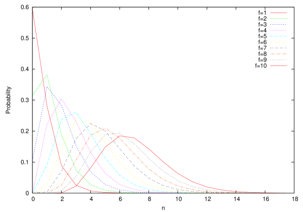
Figure 3: The distribution of sequence length for the first $10$ cycles ($f=1,2,\dots,10$) with incomplete nucleotide incorporation. The nucleotide composition probabilities used here are the same as in Figure 1. The hypothetical non-zero nucleotide incorporation probabilities are $\alpha_{{j}}^{(a)}=[6/55,1/2,3/10,1/11]$, $\alpha_{j}^{(b)}=[19/60,1/4,1/3,1/10]$, $\alpha_{j}^{(c)}=[407/630,1/7,1/10,1/9]$, and $\alpha_{j}^{(d)}=[17/40,1/5,1/4,1/8]$. The distribution is calculated from Eq. (19).

The distributions of sequence length for the first $10$ flow cycles ($f=1,2,\dots,10$) with incomplete nucleotide incorporation are show in Figure 3. The nucleotide composition probabilities used are $p_{a}=1/3=0.3333$, $p_{b}=1/11=0.0909$, $p_{c}=100/231=0.4329$, and $p_{d}=1/7=0.1429$, the same as those used for complete nucleotide incorporation case, such as Figure 1. The hypothetical non-zero nucleotide incorporation probabilities used are $\alpha_{{j}}^{(a)}=[6/55,1/2,3/10,1/11]$, $\alpha_{j}^{(b)}=[19/60,1/4,1/3,1/10]$, $\alpha_{j}^{(c)}=[407/630,1/7,1/10,1/9]$, and $\alpha_{j}^{(d)}=[17/40,1/5,1/4,1/8]$, for $j=0$, $1$, $2$, and $3$. For $j>3$, $\alpha_{j}^{(i)}=0$. The distribution is calculated from Eq. (19). These distributions can be compared with those in Figure 1 of complete nucleotide incorporation conditions.

3.3 Mean and variance

From the GF $\mathcal{G}(x,y)$ we can obtain closed form expressions of the mean and variance of the sequence length distribution using Eq. (8a) and Eq. (8b). Since $t_{1}(1)=1$, the denominator of $\left.\partial\mathcal{G}(x,y)/\partial y\right|_{y=1}$ has a $(x-1)^{2}$ factor, and the denominator of $\left.\partial^{2}\mathcal{G}(x,y)/\partial y^{2}\right|_{y=1}$ has a $(x-1)^{3}$ factor. Again $x=1$ is the pole that has the smallest module. Using the principal part of the series expansion, we get the closed form expression of the mean and variance of $P(n,f)$ as

$$\bar{n}(f)\approx\frac{f}{u}-\frac{2e_{2}^{2}-2e_{3}+4e_{2}t_{1}^{\prime}+2(t_{1}^{\prime})^{2}-t_{1}^{\prime\prime}-2t_{2}^{\prime}}{2u^{2}},$$ (20)

and

$$\sigma^{2}(f)\approx\frac{v-(3e_{2}+t_{1}^{\prime}-1)u}{u^{3}}f+\frac{w}{12u^{4}},$$ (21)

where

$$u =e_{2}+t_{1}^{\prime},$$

$$v =2e_{3}+t_{1}^{\prime\prime}+2t_{2}^{\prime},$$

$$w =6uv(3u-4e_{2})+15v^{2}-8u[3u(t_{2}^{\prime}+t_{1}^{\prime\prime})+6t_{3}^{\prime}+t_{1}^{(3)}+3t_{2}^{\prime\prime}+6e_{4}].$$

Here we use the abbreviations $t_{i}^{\prime}$ to denote $t_{i}^{\prime}(1)$, $t_{i}^{\prime\prime}$ as $t_{i}^{\prime\prime}(1)=\partial^{2}t_{i}(x)/\partial x^{2}|_{x=1}$, etc.

From Eq. (20) and Eq. (21) we see that both mean and variance are linear function of $f$. The coefficients of $f$ are the same for both FFCM and FSLM (Eq. (17a) and Eq. (17b) of Ref. Kong (2009b)). Only the constant terms differ between the two models.

In Table 5 comparisons of the closed form approximations of the mean (Eq. (20)) and the variance (Eq. (21)) against their respective exact values for the first few values of $f$ are shown, with the same parameters as those in Figure 3. The exact values are calculated from Eq. (19) using Eq. (8a) and Eq. (8b). We can see that the closed form approximations are quite close to the exact values. As $f$ increases, the errors become smaller; when $f$ reaches $f=8$, the errors become negligible.

Table 5: Comparisons of the closed form approximations of the mean (Eq. (20)) and the variance (Eq. (21)) against their respective exact values for the first few values of $f$, with the same parameters as those in Figure 3. The exact values are calculated from Eq. (19) using Eq. (8a) and Eq. (8b).

	$\bar{n}(f)$		$\sigma^{2}(f)$
$f$	Eq. (20)	exact mean	Eq. (21)	exact variance
1	0.43744094	0.57921752	0.82083681	0.72850788
2	1.17769743	1.16602712	1.29206252	1.30509385
3	1.91795391	1.89883904	1.76328823	1.80247850
4	2.65821039	2.68250622	2.23451393	2.15175889
5	3.39846688	3.39672794	2.70573964	2.71085442
6	4.13872336	4.13533479	3.17696535	3.19335924
7	4.87897985	4.88027760	3.64819106	3.64210312
8	5.61923633	5.61927551	4.11941677	4.11866116
9	6.35949281	6.35913945	4.59064248	4.59319956
10	7.09974930	7.09989881	5.06186819	5.06080288
11	7.84000578	7.84002311	5.53309389	5.53286474
12	8.58026226	8.58022040	6.00431960	6.00472717
13	9.32051875	9.32053270	6.47554531	6.47541913
14	10.06077523	10.06077853	6.94677102	6.94672379
15	10.80103172	10.80102741	7.41799673	7.41804782
16	11.54128820	11.54128938	7.88922244	7.88920999
17	12.28154468	12.28154513	8.36044814	8.36044095
18	13.02180117	13.02180070	8.83167385	8.83168045
19	13.76205765	13.76205775	9.30289956	9.30289844
20	14.50231414	14.50231420	9.77412527	9.77412416

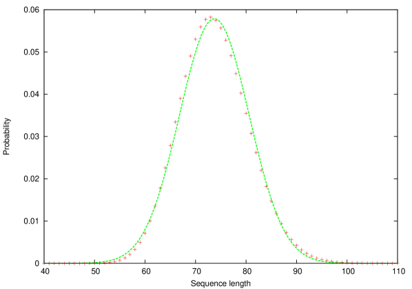
Figure 4: The distribution of sequence length with incomplete nucleotide incorporation for a fixed flow cycle of $f=100$. The nucleotide composition probabilities and the nucleotide incorporation probabilities used here are the same as in Figure 3. The exact distribution is plotted as ’+’ and is calculated from Eq. (19). The continuous curve is the normal distribution $N({\bar{n}}(f),\sigma^{2}(f))$ of the same mean and variance as those of the exact distribution, where ${\bar{n}}(f)$ and $\sigma^{2}(f)$ are calculated from Eqs. (20) and (21). The normal distribution shown here is $N(73.7228,47.4722)$.

Figure 4 shows the distribution of sequence length with incomplete nucleotide incorporation for a fixed flow cycle of $f=100$. The parameters used here are the same as in Figure 3. The exact distribution is plotted as ’+’ and is calculated from Eq. (19). The continuous curve is the normal distribution $N({\bar{n}}(f),\sigma^{2}(f))$ of the same mean and variance as those of the exact distribution, where ${\bar{n}}(f)$ and $\sigma^{2}(f)$ are calculated from Eqs. (20) and (21). The normal distribution shown here is $N(73.7228,47.4722)$. The agreement of the exact distribution with normal distribution is decent, with a slight skew to the left.

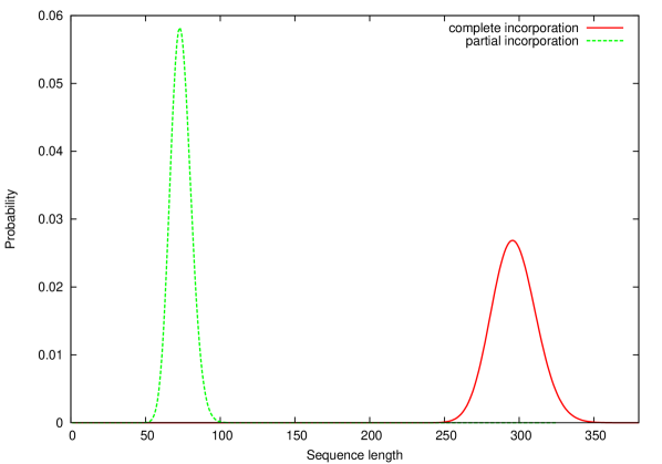
Figure 5: The distributions of sequence length for a fixed flow cycle of $f=100$ for complete and incomplete nucleotide incorporation. The curve on the right is for complete nucleotide incorporation, the curve on the left is for incomplete nucleotide incorporation. The nucleotide composition probabilities and the nucleotide incorporation probabilities are the same as in Figure 2 and Figure 4.

For comparison, the distributions of sequence length with complete and incomplete nucleotide incorporation for a fixed flow cycle of $f=100$ are shown in the same plot in Figure 5. The nucleotide composition probabilities and the nucleotide incorporation probabilities are the same as those in Figure 2 and Figure 4. The delays of synthesis in the incomplete incorporation case shift the mean of the sequence length distribution to the left, with a smaller variance.

References

- Harris et al (2008) Harris TD, Buzby PR, Babcock H, Beer E, Bowers J, Braslavsky I, Causey M, Colonell J, Dimeo J, Efcavitch WJ, Giladi E, Gill J, Healy J, Jarosz M, Lapen D, Moulton K, Quake SR, Steinmann K, Thayer E, Tyurina A, Ward R, Weiss H, Xie Z (2008) Single-molecule dna sequencing of a viral genome. Science 320(5872):106–109, DOI 10.1126/science.1150427
- Kong (2009a) Kong Y (2009a) Statistical distributions of pyrosequencing. J Comput Biol 16:31–42, DOI 10.1089/cmb.2008.0106
- Kong (2009b) Kong Y (2009b) Statistical distributions of sequencing by synthesis with probabilistic nucleotide incorporation. J Comput Biol 16:817–827, DOI 10.1089/cmb.2008.0215
- Wilf (2006) Wilf HS (2006) Generatingfunctionology. A. K. Peters, Ltd., Natick, MA, USA