How to efficiently destroy a network with limited information

Abstract

We address the general problem of how best to attack and destroy a network by node removal, given limited or no prior information about the edges. We consider a family of strategies in which nodes are randomly chosen, but not removed. Instead, a random acquaintance (i.e., a first neighbour) of the chosen node is removed from the network. By assigning an informal cost to the information about the network structure, we show using cost-benefit analysis that acquaintance removal is the optimal strategy to destroy networks efficiently.

Networks Newman (2010); Dorogovtsev and Mendes (2003); Dorogovtsev (2010); Cohen and Havlin (2010) have been used todescribe many kinds of systems Watts and Strogatz (1998); Albert et al. (1999); Jeong et al. (2000); Amaral et al. (2000); Liljeros et al. (2001); Camacho et al. (2002); Girvan and Newman (2002); Newman (2010); Dorogovtsev and Mendes (2003); Dorogovtsev (2010); Cohen and Havlin (2010). In general nodes represent system components and edges the interactions between them. How the edges are arranged in a networks has great importance because quantities of interest depend on edge placement Newman (2010); Dorogovtsev and Mendes (2003); Dorogovtsev (2010); Cohen and Havlin (2010); Newman (2008), e.g. connectivity distribution, clustering coefficient, resilience to node and edge removal, spreading processes, and small-world effects. The two most studied are networks with a typical value of connectivity and scale-free networks. In the former the edges are placed between completely random node pairs following the Erdös-Rényi (ER) algorithm Erdös and Rényi (1960). In the latter the edges are placed randomly with a bias towards more connected nodes according to the Barabási-Albert (BA) algorithm Barabási and Albert (1999). The vulnerability of network to attacks, the strategies used in these attacks and the strategies’ efficiency have been extensively studied since 2000s Callaway et al. (2000); Albert et al. (2000, 2001); Holme et al. (2002); Cohen et al. (2000, 2001, 2003); Gallos et al. (2005, 2007); Holme (2004); Bellingeri et al. (2014). A network can be attacked by removing nodes or edges. When an edge is removed, the rest of the network remains unchanged. When a node is removed, standard practice is to remove all the edges linked to the removed node. In this paper we study how to destroy ER and BA networks through node removal. Among the various ways to remove nodes, two basic forms are particularly interesting Albert et al. (2000, 2001). The random strategy consists of removing nodes randomly. The targeted strategy consists of removing nodes in order according to their connectivity, from the highest connected nodes to the lowest connected. These two strategies are limiting cases: the random strategy requires zero information about the edges, whereas the targeted strategy demands that all edges are known in advance. To target the nodes in order, one needs to know the full network structure, i.e. one needs the complete information about the network.

Apart from these two basic strategies, we present a family of strategies based on an idea introduced by Cohen et al. Cohen et al. (2003) in a different context: the acquaintance immunization strategy. The idea is as follows: instead of immunizing a randomly chosen node, it’s better to immunize a random acquaintance of the node. We refer to this as the acquaintance strategy. Compared to a single random choice, these two combined random choices increase the probability that highly connected nodes are immunized, even though their connectivity remains unknown. Here, we adapt this idea to the network destruction context.

We first explain in more detail why the acquaintance strategy works. Fig. 1 illustrates how most networks can be separated into two parts (node sets): a “center” formed by the most connected nodes and a “periphery” with all remaining nodes. There are some exceptions to this rule, such as regular networks, which we ignore here. The number of peripheral nodes is greater than the number of nodes in the center and the difference grows when the total number of nodes increases. As there are few nodes in the center and each has many edges, the vast majority of these edges connects central nodes to peripheral nodes. Similarly, each peripheral node has few edges and, on average, only a small portion connects two peripheral nodes. Hence the majority of edges of a peripheral node have a central node at the other end. The two combined random choices work together as follows: (i) the first random choice over all the nodes has greater probability of choose a peripheral node, and (ii) the second random choice over this first selected node’s acquaintances has greater probability of picking out a central node. Therefore, the acquaintance strategy is more easily capable of reaching the central nodes, compared to the random strategy. It essentially exploits the existence of edges connecting the periphery to the center.

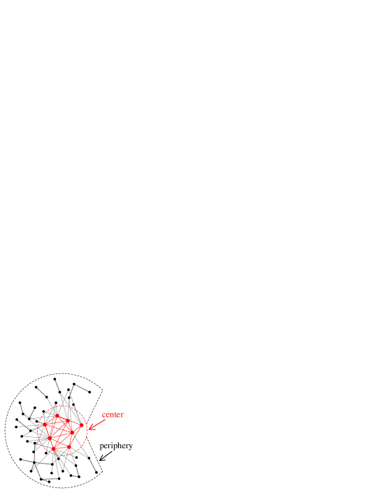
Figure 1: (Color online) Illustration of network center (red) and periphery (the remaining nodes), showing that most of the edges connect center and periphery (solid gray edges). Informally, the central nodes have much higher connectivity or degree. Independently of the rules governing the distribution of the edges in a network, random assignment or preferential attachment, the number of nodes in the center is much smaller than the number of nodes in the periphery when the total number of nodes in the network is very large. Nevertheless, the number of edges inside the center (red, dotted) and inside the periphery (black, dotted) are typically small compared to the total number of edges. The majority of edges (solid gray) connect peripheral nodes to central nodes. Key consequences are (i) when a node is randomly chosen, it is likely a peripheral node and (ii) when one of its acquaintance (or first neighbour) is randomly selected, most likely the acquaintance belongs to the center. These two facts motivate a simple strategy to destroy the center: randomly attack the acquaintances of random chosen nodes.

However, because the acquaintance strategy don’t consider node connectivity, the order in which it removes the nodes is not the best. The strategy that implements the best order for removing nodes is the targeted strategy. Seeking to upgrade the acquaintance strategy’s performance, improvements on the original idea have been proposed Holme (2004); Gallos et al. (2007), but they require knowledge of the number of edges for a given node. We take a different approach and suggest an improvement that indirectly exploits the connectivity, but does not require its direct knowledge. Specifically, we propose that a node must be chosen as an acquaintance more than once before it is removed. The basic insight is that some acquaintances are more central than others. In other words, the more edges a node has, the more likely it is chosen as an acquaintance.

We now impose a threshold $n_{r}$ for node removal. Associate to each node $j$ a memory parameter $n_{j}$. Initially all the nodes have $n_{j}=0$, but when a node is selected among the acquaintances of another randomly chosen node, it increments to $n_{j}=1$. Again if the same node is selected between the acquaintances afterwards, it increases to $n_{j}=2$, and so on. When it attains the threshold $n_{r}$, then the node is removed. A given node may be selected from the acquaintances of a same node more than once. In this approach, the original acquaintance strategy described previously corresponds to the special case $n_{r}=1$. This slight modification increases the probability that the most connected nodes are the first to be removed.

The value of the threshold $n_{r}$ thus generates a whole family of acquaintance strategies, such that each strategy is characterized by a specific value for the removal threshold $n_{r}$. The number of nodes that must be removed to destroy a network resulting from the application of all the mentioned strategies is shown in Fig. 2. While plots A and B show how the network’s largest cluster loses nodes when a network is attacked, plots C and D show how the largest cluster loses edges at the same time. In summary, these plots have a clear interpretation: even though acquaintance strategies are based on only two combined random choices, they can destroy a network faster than the random strategy. Moreover, they have better performance on BA rather than ER networks. The plots also confirm that the memory parameter represents an improvement on the original acquaintance idea, because the acquaintance curves deviate from the random strategy curve and approach the targeted strategy curve for higher $n_{r}$.

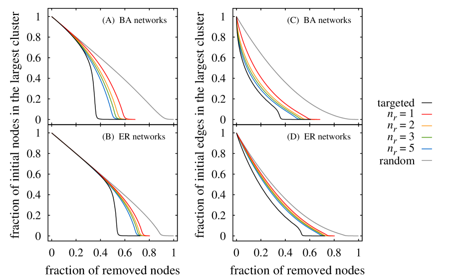
Figure 2: (Color online) Attacking randomly chosen acquaintances is more destructive than attacking the original randomly chosen nodes. Plots show the fraction of initial nodes remaining in the largest cluster after attack (plots A and B), and similarly the fraction of remaining initial edges (plots C and D). For all the plots, the leftmost curve corresponds to the targeted strategy, the rightmost corresponds to the random strategy. The four middle curves refer to the family of acquaintance strategies, in which every node has a parameter $n_{j}$ that counts how many times it has been selected as an acquaintance. Each particular strategy has a defined threshold $n_{r}$ such that when a node has $n_{j}=n_{r}$, it is removed. From left to right: acquaintance curves for $n_{r}=5$, $n_{r}=3$, $n_{r}=2$ and the simple acquaintance case with $n_{r}=1$. Erdös-Rényi (ER) networks are more resistant in general than Barabási-Albert (BA) networks. But BA networks are slightly less fragile to the random strategy. Remembering that each removed node carries away the edges connected to it, the curves in plots C and D reveal how the removing order of nodes for each strategy is closer to the best order (targeted strategy). So, the faster the curve falls, the more connected were the removed nodes. We consider that the network is destroyed when there are no edges connecting the nodes that haven’t been removed yet, so the curves extends only to this point. This same pattern plot is kept for all the other graphs. These results, and all others hereafter, are based on simulation of 100 networks of each type and each network has 10000 nodes and 49985 edges.

Thus far, we have shown the damage to the largest cluster when we remove a given fraction of nodes (Fig. 2). However, this is just one aspect of the efficiency. How much information about a network do we need access to remove a given fraction of nodes using each strategy? Considering that the information about the structure of a network is contained in the edges, we attributed to knowledge of each edge an informal information cost. We consider only networks with simple unweighted edges, so that the same cost is assigned to every edge. Thus the total cost associated to the execution of each strategy is given by the number of edges known during the node removal process. In Fig. 3 this issue is examined and the plots highlight the cost of information: the random and targeted strategies are limiting cases, the former having zero cost associated and the latter having maximum possible cost. The family of acquaintance strategies has a cost proportional to the characteristic $n_{r}$ of each particular strategy, so that the acquaintance strategy without memory is that with minor cost between them. In fact, the execution of the original acquaintance idea has a cost with linear growth during all the removing process, which makes this strategy optimal if we only take into account the cost-dependent aspect (because for each edge known, one node is removed). It’s noteworthy that the acquaintance strategies don’t require any prior information about the networks, they are such that as soon as information is acquired, it can be immediately used for node removal.

A complete analysis of efficiency only can be done when the plots shown in Figs. 2 and 3 are considered altogether. Unfortunately a direct way to do this analysis doesn’t exist and we can do it only qualitatively. Indeed, the appropriate strategy depends on the availability of information about the network to be destroyed. If the network can be examined in all its extension, such that all the information about it is available, the appropriate strategy is to attack from the most connected nodes, i.e. the targeted strategy. If only a limited amount of information can be accessed, then a balance between the number of edges that can be known and the number of nodes that should be removed until the network destruction must be considered. In this case one of the acquaintance strategies is most appropriate.

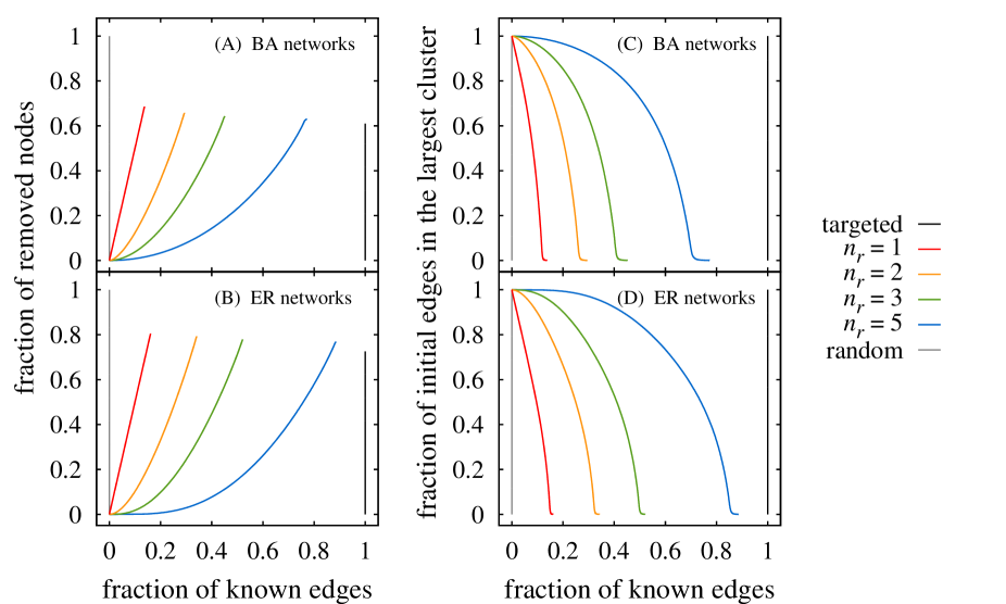
Figure 3: (Color online) Analysis of the informal cost involving in attacking a network following one of the cited strategies. Plots show the fraction of removed nodes (plots A and B) and the fraction of initial nodes remaining in the largest cluster (plots C and D) in relation to the informal cost, that is, the number of edges that need to be known at that moment. For all the plots, the curves from left to right are: random, $n_{r}=1$, $n_{r}=2$, $n_{r}=3$, $n_{r}=5$ and targeted curves, using the same nomenclature of Fig. 2. The targeted strategy (vertical line at left) and the random strategy (vertical line at right) are limiting cases: the former requires that all the edges be known, while the latter can be carried out without any edge be known. Between these two there is a family of curves relative to the acquaintance strategy. The basic acquaintance removal ($n_{r}=1$) demands that only a small fraction of the edges be known. This is a demonstration that the acquaintance strategy without memory parameter is efficient from the viewpoint of the number of edges that must to be accessed before a network be destroyed. However by this viewpoint, when the memory parameter is considered, more edges need to be known and this aspect of the efficiency is progressively lost. It’s worth noting that the less nodes a strategy removes until destroying a network, the more costly it is.

We comment on a secondary finding. The fragility of BA networks to attacks is evident when compared to ER networks, except for the random strategy. Even in this case, the difference in favour of BA networks only can be noted when most of the nodes have already been removed. Consider strategies which aim to destroy networks from the central nodes. Fig. 3 shows that the cost involved in executing each strategy is almost the same for both types of networks, yet BA networks are highly susceptible to the loss of edges, according to plots C and D in Fig. 2, and their largest clusters break up faster, according to plots A and B. This is a consequence of the form in which information about the structure of the networks, i.e. the edges, is distributed between the nodes. This point deserves a further discussion.

When the same strategy is used to attack networks of different types, the fragilities of each type will determine how efficient the strategy is. For example, ER networks don’t have a well-defined lower limit for the connectivity of its nodes allowing that some nodes have only one edge linked to them, so that the removal of these nodes can break the networks into fragments. However, these fragments will preserve a good part of the network because very few edges have been lost with the removed nodes. Furthermore, it is hard to reach these nodes, since they have very few neighbours, which allows the random strategy to reach them more efficiently than a connectivity-driven strategy. In other words, the information about the network is dispersed over its entire extent. In contrast, BA networks have a fundamental fragility: the existence of extremely connected nodes. They are few, but they concentrate a great number of edges around them. Any information about the structure of these networks points to the same regions, to the same nodes. So, the removal of these hubs can weaken the network, sometimes to the point at which it will quickly become fragmented into tiny pieces. In this case the information about the network is concentrated around a few regions, rendering the network more susceptible to strategies that exploit connectivity, even indirectly, such as the acquaintance strategies studied here.