Relativistic third-order viscous corrections to the entropy four-current from kinetic theory

Abstract

By employing a Chapman-Enskog like iterative solution of the Boltzmann equation in relaxation-time approximation, we derive a new expression for the entropy four-current up to third order in gradient expansion. We show that unlike second-order and third-order entropy four-current obtained using Grad’s method, there is a non-vanishing entropy flux in the present third-order expression. We further quantify the effect of the higher-order entropy density in the case of boost-invariant one-dimensional longitudinal expansion of a system. We demonstrate that the results obtained using third-order evolution equation for shear stress tensor, derived by employing the method of Chapman-Enskog expansion, show better agreement with the exact solution of the Boltzmann equation as well as with the parton cascade BAMPS, as compared to those obtained using the third-order equations from the method of Grad’s 14-moment approximation.

I Introduction

Study of the space-time evolution and non-equilibrium properties of hot and dense matter produced in high-energy heavy-ion collisions, within the framework of relativistic viscous hydrodynamics, has gained widespread interest; see Ref. Heinz:2013th for a recent review. Hydrodynamics is an effective theory that describes the long-wavelength limit of the microscopic dynamics of a system. As a macroscopic theory which describes the space-time evolution of the energy-momentum tensor, it is much less involved than microscopic descriptions such as kinetic theory. In order to study the hydrodynamic evolution of a system, it is natural to first employ the equations of ideal hydrodynamics. However, ideal hydrodynamics is based on the unrealistic assumption of local thermodynamic equilibrium which results in isentropic evolution. Moreover, since the quantum mechanical uncertainty principle provides a lower bound on the shear viscosity to entropy density ratio Danielewicz:1984ww ; Kovtun:2004de , the dissipative effects can not be ignored.

Eckart Eckart:1940zz and Landau and Lifshitz Landau were the first to formulate a relativistic theory of dissipative hydrodynamics, each with a different choice for the definition of hydrodynamic four-velocity. These theories are based on the assumption that the entropy four-current is linear in dissipative quantities and hence they are also known as first-order theories of dissipative fluids. The resulting equations for the dissipative quantities are essentially the relativistic analogue of the Navier-Stokes equations. However, the resulting equations of motion lead to parabolic differential equations which suffer from acausality and numerical instability. In order to rectify the undesirable features of first-order theories, extended theories of dissipative fluids were introduced by Grad Grad , Müller Muller:1967zza and Israel and Stewart Israel:1979wp . These theories are based on the assumption that the entropy four-current contains terms quadratic in the dissipative fluxes and therefore are also known as second-order theories. The resulting equations of motion are hyperbolic in nature which preserves causality Huovinen:2008te but may not guarantee stability.

Second-order Israel-Stewart (IS) hydrodynamics has been quite successful in explaining a wide range of collective phenomena observed in ultra-relativistic heavy-ion collisions Heinz:2013th . Despite its successes, the formulation of IS theory is based on certain approximations and assumptions. For instance, the original IS theory employs an arbitrary choice of the second moment of the Boltzmann equation to obtain the equations of motion for the dissipative currents Israel:1979wp . Another assumption inherent in IS theory is the use of Grad’s 14-moment approximation for the non-equilibrium distribution function Grad ; Israel:1979wp . Moreover, the IS theory is a second-order theory which neglects contributions from higher-order terms in the entropy four-current. It is thus of interest to extend the second-order theory beyond its present scope and determine the associated transport coefficients for a hydrodynamic system.

In a non-equilibrium system, the presence of thermodynamic gradients results in thermodynamic forces which in turn gives rise to various transport phenomena. Therefore transport coefficients such as viscosity, diffusivity and conductivity, are important to characterize the dynamics of a system. Precise knowledge of these transport coefficients and associated length and time scales is necessary in comparing observables with theoretical predictions. In order to calculate these transport coefficients from the underlying kinetic theory, it is convenient to first determine the non-equilibrium single particle phase-space distribution function $f(x,p)$. When the system is close to local thermodynamic equilibrium, two most commonly used methods to determine the form of $f(x,p)$ are (1) Grad’s 14-moment approximation Grad and (2) the Chapman-Enskog expansion Chapman . Although both methods involve expanding $f(x,p)$ around its equilibrium value $f_{0}(x,p)$, in Refs. Jaiswal:2013npa ; Jaiswal:2013vta ; Jaiswal:2014isa it was shown that the Chapman-Enskog method in the relaxation-time approximation (RTA) gives better agreement with microscopic Boltzmann simulations as well as exact solutions of the RTA Boltzmann equation. Consistent derivation of the form of the dissipative equations and accurate determination of the associated transport coefficients is still an active research area Jaiswal:2013npa ; Jaiswal:2013vta ; Jaiswal:2014isa ; Muronga:2003ta ; Denicol:2010xn ; York:2008rr ; Denicol:2012cn ; Jaiswal:2012qm ; Jaiswal:2013fc ; Bhalerao:2013aha ; Bhalerao:2013pza ; Martinez:2010sc ; Martinez:2012tu ; Florkowski:2013lza ; Bazow:2013ifa ; El:2009vj ; Muronga:2010zz ; Muronga:2014yua ; Denicol:2014mca ; Florkowski:2010cf ; Florkowski:2014sfa .

In this paper, we derive a new expression for the entropy four-current up to third-order in dissipative fluxes by employing the Chapman-Enskog expansion for the non-equilibrium distribution function. Although third-order expressions for entropy four-current have been derived using Grad’s 14-moment approximation El:2009vj ; Muronga:2010zz ; Muronga:2014yua , we present here, for the first time, the derivation using the Chapman-Enskog method. We show that unlike second-order and third-order results from Grad’s method, there is a non-vanishing entropy flux (projection of the entropy four-current orthogonal to the fluid four-velocity) in our expression for the entropy four-current. We demonstrate the significance of the present derivation in the special case of a system undergoing boost-invariant Bjorken expansion. We show that compared to the Grad’s method, the Chapman-Enskog method is able to reproduce better the exact solution of Boltzmann equation Florkowski:2013lza ; Baym:1984np as well as the BAMPS results El:2009vj ; Xu:2004mz .

II Iterative solution of the Boltzmann equation

Evolution of the single particle phase-space distribution function, $f(x,p)$, is governed by the Boltzmann equation. In the absence of collisions, the particles propagate along geodesics which implies that $f(x,p)$ does not change along geodesics. Therefore for a geodesic parametrized by an affine parameter $\Lambda$, we have $df/d\Lambda=0$. When collisions are present, particles will no longer move along geodesics leading to a non-vanishing $df/d\Lambda$. Hence, in general, one can write the Boltzmann equation as

$$p^{\mu}\partial_{\mu}f+F^{\mu}\partial_{\mu}^{(p)}f={\cal C}[f],$$ (1)

where $p^{\mu}$ is the particle four-momentum, $F^{\mu}$ is the external force felt by the particles and ${\cal C}[f]$ is the collision functional.

In absence of any external forces and using the relaxation-time approximation for the collision term, Eq. (1) can be rewritten as Anderson_Witting

$$p^{\mu}\partial_{\mu}f=-(u\cdot p)\frac{\delta f}{\tau_{R}},$$ (2)

where $u\cdot p\equiv u_{\mu}p^{\mu}$, $\tau_{R}$ is the relaxation time and $\delta f\equiv f-f_{0}$ is the non-equilibrium part of the distribution function, $f_{0}$ being the equilibrium distribution function. In the following, we consider only classical massless particles obeying the Boltzmann statistics at vanishing chemical potential, i.e., $f_{0}=\exp(-\beta\,u\cdot p)$, where $\beta\equiv 1/T$ is the inverse temperature.

Equation (2) can be solved iteratively to obtain a Chapman-Enskog like expansion for the non-equilibrium part of the distribution function in powers of space-time gradients Chapman ; Romatschke:2011qp

$$\delta f=\delta f^{(1)}+\delta f^{(2)}+\delta f^{(3)}+\cdots,$$ (3)

where $\delta f^{(1)}$ is first-order in derivatives, $\delta f^{(2)}$ is second-order and so on. To first- and second-order in derivatives, one obtains

$$\delta f^{(1)} =-\frac{\tau_{R}}{u\!\cdot\!p}\,p^{\mu}\partial_{\mu}f_{0},$$ (4)

$$\delta f^{(2)} =\frac{\tau_{R}}{u\!\cdot\!p}p^{\mu}p^{\nu}\partial_{\mu}\Big{(}\frac{\tau_{R}}{u\!\cdot\!p}\partial_{\nu}f_{0}\Big{)}.$$ (5)

Derivation of hydrodynamic evolution equations for dissipative quantities within the framework of kinetic theory requires the form of $\delta f$ to be specified. In the following, we employ Eq. (3) along with Eqs. (4) and (5) to specify the non-equilibrium distribution function.

III Relativistic viscous hydrodynamics

The hydrodynamic evolution of a relativistic system, in absence of any conserved charges, is governed by the conservation equation of the energy-momentum tensor. In terms of the phase-space distribution function and hydrodynamic variables, the conserved energy-momentum tensor can be expressed as deGroot

$$T^{\mu\nu} =\!\int\!dp\ p^{\mu}p^{\nu}\,f(x,p)=\epsilon u^{\mu}u^{\nu}-P\Delta^{\mu\nu}+\pi^{\mu\nu},$$ (6)

where $dp\equiv gd{\bf p}/[(2\pi)^{3}|\bf p|]$, $g$ being the degeneracy factor, $\epsilon$, $P$ and $\pi^{\mu\nu}$ are respectively energy density, pressure and the shear stress tensor. For a system of massless particles the bulk viscous pressure vanishes. The projection operator $\Delta^{\mu\nu}\equiv g^{\mu\nu}-u^{\mu}u^{\nu}$ is orthogonal to the hydrodynamic four-velocity $u^{\mu}$ defined in the Landau frame: $T^{\mu\nu}u_{\nu}=\epsilon u^{\mu}$. We consider the metric tensor to be Minkowskian, i.e., $g^{\mu\nu}\equiv\mathrm{diag}(+,-,-,-)$.

The evolution equations for $\epsilon$ and $u^{\mu}$ are obtained from the fundamental energy-momentum conservation, $\partial_{\mu}T^{\mu\nu}=0$,

$$\dot{\epsilon}+(\epsilon+P)\theta-\pi^{\mu\nu}\sigma_{\mu\nu} =0,$$ (7)

$$(\epsilon+P)\dot{u}^{\alpha}-\nabla^{\alpha}P+\Delta^{\alpha}_{\nu}\partial_{\mu}\pi^{\mu\nu} =0.$$ (8)

We use the standard notation $\dot{A}\equiv u^{\mu}\partial_{\mu}A$ for co-moving derivative, $\theta\equiv\partial_{\mu}u^{\mu}$ for the expansion scalar, $\sigma_{\mu\nu}\equiv(\nabla_{\mu}u_{\nu}+\nabla_{\nu}u_{\mu})/2-(\theta/3)\Delta_{\mu\nu}$ for velocity stress tensor and $\nabla^{\alpha}\equiv\Delta^{\mu\alpha}\partial_{\mu}$ for space-like derivative. In the conformal limit, the energy density and pressure are related through $\epsilon=3P\propto\beta^{-4}$, where the inverse temperature $\beta\equiv 1/T$ is defined using the equilibrium matching condition $\epsilon=\epsilon_{0}$. In this limit the derivatives of $\beta$ can be obtained using Eqs. (7) and (8)

$$\dot{\beta} =\frac{\beta}{3}\theta-\frac{\beta}{12P}\pi^{\rho\gamma}\sigma_{\rho\gamma},$$ (9)

$$\nabla^{\alpha}\beta =\!-\beta\dot{u}^{\alpha}-\frac{\beta}{4P}\Delta^{\alpha}_{\rho}\partial_{\gamma}\pi^{\rho\gamma}.$$ (10)

In the following, we will employ the above identities to derive the form of dissipative corrections to the distribution function as well as the evolution equation for shear stress tensor.

In terms of $\delta f$, shear stress tensor ($\pi^{\mu\nu}$) can be expressed as

$$\pi^{\mu\nu} =\Delta^{\mu\nu}_{\alpha\beta}\int dp\,p^{\alpha}p^{\beta}\,\delta f,$$ (11)

where $\Delta^{\mu\nu}_{\alpha\beta}\equiv\Delta^{\mu}_{(\alpha}\Delta^{\nu}_{\beta)}-(1/3)\Delta^{\mu\nu}\Delta_{\alpha\beta}$ is a traceless symmetric projection operator orthogonal to $u^{\mu}$. The first-order expression for shear stress tensor can be obtained from Eq. (11) using $\delta f=\delta f^{(1)}$ from Eq. (4),

$$\pi^{\mu\nu} =\Delta^{\mu\nu}_{\alpha\beta}\int dp\ p^{\alpha}p^{\beta}\left(-\frac{\tau_{R}}{u\!\cdot\!p}\,p^{\mu}\partial_{\mu}\,f_{0}\right).$$ (12)

Using Eqs. (9) and (10), and retaining terms which are first-order in gradients, the integrals in the above equation reduce to

$$\pi^{\mu\nu}=2\tau_{R}\beta_{\pi}\sigma^{\mu\nu},$$ (13)

where $\beta_{\pi}=4P/5$.

In order to obtain higher-order evolution equations, we consider the co-moving derivative of Eq. (11),

$$\dot{\pi}^{\langle\mu\nu\rangle}=\Delta^{\mu\nu}_{\alpha\beta}\int dp\,p^{\alpha}p^{\beta}\,\delta\dot{f},$$ (14)

where we have used the notation $A^{\langle\mu\nu\rangle}\equiv\Delta^{\mu\nu}_{\alpha\beta}A^{\alpha\beta}$ for traceless symmetric projection orthogonal to $u^{\mu}$. The co-moving derivative of the non-equilibrium part of the distribution function, $\delta\dot{f}$, can be obtained by rewriting Eq. (2) in the form Denicol:2010xn

$$\delta\dot{f}=-\dot{f}_{0}-\frac{1}{u\!\cdot\!p}p^{\gamma}\nabla_{\gamma}f-\frac{\delta f}{\tau_{R}}.$$ (15)

Using this expression for $\delta\dot{f}$ in Eq. (14), we obtain

$$\dot{\pi}^{\langle\mu\nu\rangle}+\frac{\pi^{\mu\nu}}{\tau_{R}}=-\Delta^{\mu\nu}_{\alpha\beta}\!\int\!\frac{dp}{u\!\cdot\!p}\,p^{\alpha}p^{\beta}p^{\gamma}\nabla_{\gamma}f.$$ (16)

From the above equation, we can conclude that the shear relaxation time $\tau_{\pi}$ is equal to the Boltzmann relaxation time $\tau_{R}$. A comparison of the first-order evolution equation, Eq. (13), with the relativistic Navier-Stokes equation, $\pi^{\mu\nu}=2\eta\sigma^{\mu\nu}$, results in $\tau_{\pi}=\eta/\beta_{\pi}$ for the shear relaxation time.

To derive the second-order evolution equation for $\pi^{\mu\nu}$, we substitute $\delta f^{(1)}$ from Eq. (4) in Eq. (16) and use Eqs. (9) and (10) for derivatives of $\beta$. We finally obtain Jaiswal:2013npa

$$\dot{\pi}^{\langle\mu\nu\rangle}\!+\frac{\pi^{\mu\nu}}{\tau_{\pi}}\!=2\beta_{\pi}\sigma^{\mu\nu}\!+2\pi_{\gamma}^{\langle\mu}\omega^{\nu\rangle\gamma}\!-\frac{10}{7}\pi_{\gamma}^{\langle\mu}\sigma^{\nu\rangle\gamma}\!-\frac{4}{3}\pi^{\mu\nu}\theta,$$ (17)

where $\omega^{\mu\nu}\equiv(\nabla^{\mu}u^{\nu}-\nabla^{\nu}u^{\mu})/2$ is the vorticity tensor. We observe that by employing the above equation, $\delta f$ in Eqs. (3)-(5) can be expressed in terms of derivatives of hydrodynamic variables up to second order. To this end, we write

$$\delta f=f_{0}\phi=f_{0}\left(\phi_{1}+\phi_{2}\right)+{\cal O}(\delta^{3}),$$ (18)

where $\phi_{1}$ and $\phi_{2}$ are first- and second-order corrections, respectively, and are calculated to be

$$\phi_{1}=\, \frac{\beta}{2\beta_{\pi}(u\!\cdot\!p)}\,p^{\alpha}p^{\beta}\pi_{\alpha\beta},$$ (19)

$$\phi_{2}=\, \frac{\beta}{\beta_{\pi}}\bigg{[}\frac{5}{14\beta_{\pi}(u\!\cdot\!p)}\,p^{\alpha}p^{\beta}\pi^{\gamma}_{\alpha}\,\pi_{\beta\gamma}-\frac{\tau_{\pi}}{u\!\cdot\!p}\,p^{\alpha}p^{\beta}\pi^{\gamma}_{\alpha}\,\omega_{\beta\gamma}$$

$$-\frac{(u\!\cdot\!p)}{70\beta_{\pi}}\,\pi^{\alpha\beta}\pi_{\alpha\beta}+\frac{6\tau_{\pi}}{5}\,p^{\alpha}\dot{u}^{\beta}\pi_{\alpha\beta}-\frac{\tau_{\pi}}{5}\,p^{\alpha}\!\left(\nabla^{\beta}\pi_{\alpha\beta}\!\right)$$

$$-\frac{\tau_{\pi}}{2(u\!\cdot\!p)^{2}}\,p^{\alpha}p^{\beta}p^{\gamma}\!\left(\nabla_{\gamma}\pi_{\alpha\beta}\!\right)+\frac{3\tau_{\pi}}{(u\!\cdot\!p)^{2}}\,p^{\alpha}p^{\beta}p^{\gamma}\pi_{\alpha\beta}\dot{u}_{\gamma}$$

$$-\frac{\tau_{\pi}}{3(u\!\cdot\!p)}\,p^{\alpha}p^{\beta}\pi_{\alpha\beta}\theta+\frac{\beta+(u\!\cdot\!p)^{-1}}{4(u\!\cdot\!p)^{2}\beta_{\pi}}\left(p^{\alpha}p^{\beta}\pi_{\alpha\beta}\right)^{2}\bigg{]}.$$ (20)

Here we have used Eqs. (9), (10) and (17) to substitute for the derivatives of $\beta$ and $u^{\mu}$. We observe that the form of $\phi_{1}$ and $\phi_{2}$ in Eqs. (19)-(20) satisfies the matching condition $\epsilon=\epsilon_{0}$ and the Landau frame definition $u_{\nu}T^{\mu\nu}=\epsilon u^{\mu}$ and is also consistent with Eq. (11) for the definition of the shear stress tensor Bhalerao:2013pza . Note that the form of $\delta f$ obtained by Denicol et. al. Denicol:2012cn , where they generalize the 14-moment method to include all terms in the moment expansion, also satisfies these conditions. However, unlike Eq. (20), the $\delta f$ obtained in Ref. Denicol:2012cn is linear in hydrodynamic gradients.

The third-order evolution equation for the shear stress tensor can also be derived by substituting $f=f_{0}(1+\phi_{1}+\phi_{2})$ in Eq. (16). After straightforward but tedious algebra, we obtain Jaiswal:2013vta

$$\dot{\pi}^{\langle\mu\nu\rangle}= -\frac{\pi^{\mu\nu}}{\tau_{\pi}}+2\beta_{\pi}\sigma^{\mu\nu}+2\pi_{\gamma}^{\langle\mu}\omega^{\nu\rangle\gamma}-\frac{10}{7}\pi_{\gamma}^{\langle\mu}\sigma^{\nu\rangle\gamma}$$

$$-\frac{4}{3}\pi^{\mu\nu}\theta+\frac{25}{7\beta_{\pi}}\pi^{\rho\langle\mu}\omega^{\nu\rangle\gamma}\pi_{\rho\gamma}-\frac{1}{3\beta_{\pi}}\pi_{\gamma}^{\langle\mu}\pi^{\nu\rangle\gamma}\theta$$

$$-\frac{38}{245\beta_{\pi}}\pi^{\mu\nu}\pi^{\rho\gamma}\sigma_{\rho\gamma}-\frac{22}{49\beta_{\pi}}\pi^{\rho\langle\mu}\pi^{\nu\rangle\gamma}\sigma_{\rho\gamma}$$

$$-\frac{24}{35}\nabla^{\langle\mu}\left(\pi^{\nu\rangle\gamma}\dot{u}_{\gamma}\tau_{\pi}\right)+\frac{4}{35}\nabla^{\langle\mu}\left(\tau_{\pi}\nabla_{\gamma}\pi^{\nu\rangle\gamma}\right)$$

$$-\frac{2}{7}\nabla_{\gamma}\left(\tau_{\pi}\nabla^{\langle\mu}\pi^{\nu\rangle\gamma}\right)+\frac{12}{7}\nabla_{\gamma}\left(\tau_{\pi}\dot{u}^{\langle\mu}\pi^{\nu\rangle\gamma}\right)$$

$$-\frac{1}{7}\nabla_{\gamma}\left(\tau_{\pi}\nabla^{\gamma}\pi^{\langle\mu\nu\rangle}\right)+\frac{6}{7}\nabla_{\gamma}\left(\tau_{\pi}\dot{u}^{\gamma}\pi^{\langle\mu\nu\rangle}\right)$$

$$-\frac{2}{7}\tau_{\pi}\omega^{\rho\langle\mu}\omega^{\nu\rangle\gamma}\pi_{\rho\gamma}-\frac{2}{7}\tau_{\pi}\pi^{\rho\langle\mu}\omega^{\nu\rangle\gamma}\omega_{\rho\gamma}$$

$$-\frac{10}{63}\tau_{\pi}\pi^{\mu\nu}\theta^{2}+\frac{26}{21}\tau_{\pi}\pi_{\gamma}^{\langle\mu}\omega^{\nu\rangle\gamma}\theta.$$ (21)

We compare the above equation with that obtained in Ref. El:2009vj using Grad’s 14-moment approximation,

$$\dot{\pi}^{\langle\mu\nu\rangle}= -\frac{\pi^{\mu\nu}}{\tau_{\pi}^{\prime}}+2\beta_{\pi}^{\prime}\sigma^{\mu\nu}-\frac{4}{3}\pi^{\mu\nu}\theta+\frac{5}{36\beta_{\pi}^{\prime}}\pi^{\mu\nu}\pi^{\rho\gamma}\sigma_{\rho\gamma}$$

$$-\frac{16}{9\beta_{\pi}^{\prime}}\pi^{\langle\mu}_{\gamma}\pi^{\nu\rangle\gamma}\theta,$$ (22)

where $\beta_{\pi}^{\prime}=2P/3$ and $\tau_{\pi}^{\prime}=\eta/\beta_{\pi}^{\prime}$. Note that the right-hand side of the above equation contains one second-order and two third-order terms compared to three second-order and fourteen third-order terms obtained in Eq. (III).

IV Entropy four-current

A well established framework for the study of thermalization processes in a system begins from the observation that thermal equilibrium corresponds to the state of maximum entropy. The interpretation of how entropy is generated in any process depends on the theoretical and conceptual framework in which the processes that lead to thermalization are described. For instance, in a relativistic system, local entropy generation is given by the divergence of the entropy four-current. For kinetic theory, the expression for entropy four-current generalized from the Boltzmann’s H-function is given by

$$S^{\mu}=-\int dp~{}p^{\mu}f\left(\ln f-1\right).$$ (23)

For a system which is close to local thermodynamic equilibrium, $f=f_{0}(1+\phi)$, where $\phi\ll 1$, we obtain an expression for the non-equilibrium entropy four-current up to third-order in $\phi$ as

$$S^{\mu}=s_{0}u^{\mu}-\int dp~{}p^{\mu}f_{0}\left(\frac{\phi^{2}}{2}-\frac{\phi^{3}}{6}\right),$$ (24)

where $s_{0}=\beta(\epsilon+P)$ is the equilibrium entropy density. For $\phi=\phi_{1}+\phi_{2}$, we have

$$S^{\mu}=s_{0}u^{\mu}-\int dp~{}p^{\mu}f_{0}\left(\frac{\phi_{1}^{2}}{2}+\phi_{1}\phi_{2}-\frac{\phi_{1}^{3}}{6}\right),$$ (25)

where we have ignored terms which are higher than third-order in derivative expansion.

Substituting $\phi_{1}$ and $\phi_{2}$ from Eqs. (19) and (20) and performing the integrations, we get

$$S^{\mu}= ~{}s_{0}u^{\mu}-\frac{\beta}{4\beta_{\pi}}\pi^{\alpha\beta}\pi_{\alpha\beta}u^{\mu}-\frac{5\beta}{42\beta_{\pi}^{2}}\pi_{\alpha\gamma}\pi^{\gamma}_{\beta}\pi^{\alpha\beta}u^{\mu}$$

$$~{}+\!\frac{\beta\tau_{\pi}}{7\beta_{\pi}}\bigg{[}\frac{18}{5}\dot{u}^{\rho}\pi_{\rho\gamma}\pi^{\mu\gamma}\!+\frac{2}{5}\pi^{\mu\gamma}\nabla^{\rho}\pi_{\rho\gamma}\!-\frac{1}{2}\pi^{\alpha\beta}\nabla^{\mu}\pi_{\alpha\beta}$$

$$~{}+3\dot{u}^{\mu}\pi_{\alpha\beta}\pi^{\alpha\beta}-\pi^{\alpha\gamma}\Delta^{\mu\rho}\nabla_{\alpha}\pi_{\rho\gamma}\bigg{]},$$ (26)

where we recall that $\beta_{\pi}=4P/5$. We compare our above result with that obtained using Grad’s 14-moment approximation El:2009vj ,

$$S^{\prime\mu}=s_{0}u^{\mu}-\frac{\beta}{4\beta_{\pi}^{\prime}}\pi^{\alpha\beta}\pi_{\alpha\beta}u^{\mu}-\frac{2\beta}{9\beta_{\pi}^{\prime 2}}\pi_{\alpha\gamma}\pi^{\gamma}_{\beta}\pi^{\alpha\beta}u^{\mu},$$ (27)

where $\beta_{\pi}^{\prime}=2P/3$. The entropy density, $s\equiv u_{\mu}S^{\mu}$, for the two cases is given by

$$s= ~{}s_{0}-\frac{\beta}{4\beta_{\pi}}\pi^{\alpha\beta}\pi_{\alpha\beta}-\frac{5\beta}{42\beta_{\pi}^{2}}\pi_{\alpha\gamma}\pi^{\gamma}_{\beta}\pi^{\alpha\beta},$$ (28)

$$s^{\prime}= ~{}s_{0}-\frac{\beta}{4\beta_{\pi}^{\prime}}\pi^{\alpha\beta}\pi_{\alpha\beta}-\frac{2\beta}{9\beta_{\pi}^{\prime 2}}\pi_{\alpha\gamma}\pi^{\gamma}_{\beta}\pi^{\alpha\beta},$$ (29)

whereas the entropy flux, $S^{\langle\mu\rangle}\equiv\Delta^{\mu}_{\nu}S^{\nu}$, in the two cases reduce to

$$S^{\langle\mu\rangle}= ~{}\frac{\beta\tau_{\pi}}{7\beta_{\pi}}\bigg{[}\frac{18}{5}\dot{u}^{\rho}\pi_{\rho\gamma}\pi^{\mu\gamma}\!+\frac{2}{5}\pi^{\mu\gamma}\nabla^{\rho}\pi_{\rho\gamma}\!-\frac{1}{2}\pi^{\alpha\beta}\nabla^{\mu}\pi_{\alpha\beta}$$

$$+3\dot{u}^{\mu}\pi_{\alpha\beta}\pi^{\alpha\beta}-\pi^{\alpha\gamma}\Delta^{\mu\rho}\nabla_{\alpha}\pi_{\rho\gamma}\bigg{]},$$ (30)

$$S^{\prime\langle\mu\rangle}= ~{}0.$$ (31)

We observe that even for vanishing bulk viscosity and dissipative charge current, Chapman-Enskog method leads to non-vanishing entropy flux as opposed to the method based on Grad’s 14-moment approximation. This may be attributed to the fact that the entropy four-current obtained in the Chapman-Enskog method contains terms proportional to acceleration $\dot{u}^{\mu}$ and gradient of shear stress tensor $\nabla^{\mu}\pi_{\alpha\beta}$. Both these quantities, as well as $\pi_{\alpha\beta}$, are orthogonal to the fluid four-velocity $u^{\mu}$ and therefore their combination results in non-vanishing entropy flux. Note that for a system with vanishing entropy flux, the entropy four-flow is entirely due to the flow of entropy density. In the case of Chapman-Enskog method, the non-vanishing entropy flux implies that the entropy density of the system should be lower than in the case of vanishing entropy flux (Grad’s method).

V Numerical results and discussion

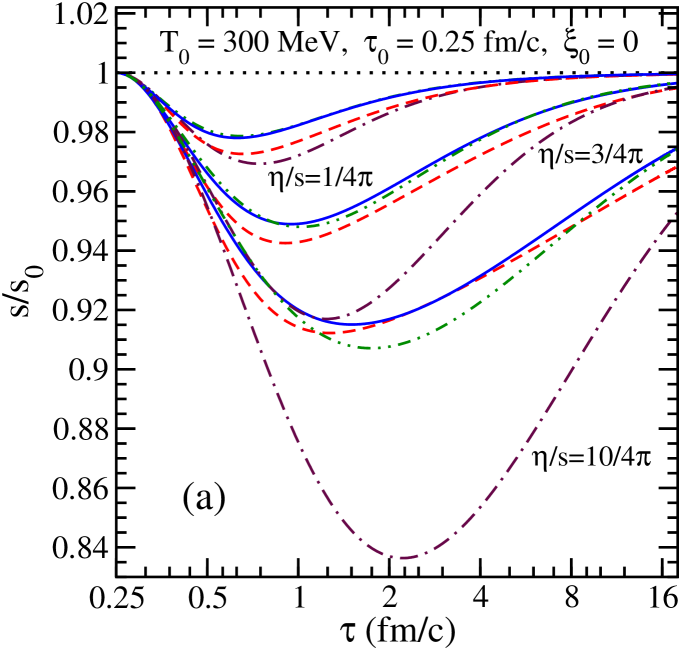
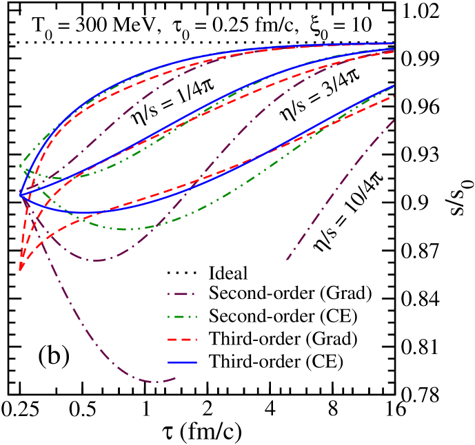
Figure 1: (Color online) Time evolution of $s/s_{0}$ obtained using ideal hydrodynamics (black dotted lines), second-order Grad’s approximation (maroon dashed-dotted lines), second-order Chapman-Enskog method (green dashed-dotted-dotted lines), third-order Grad’s approximation (red dashed lines), and third-order Chapman-Enskog method (blue solid lines) for initial temperature $T_{0}=300$ MeV at initial time $\tau_{0}=0.25$ fm/c, various $\eta/s$ and for (a): isotropic initial pressure configuration $\xi_{0}=0$ and (b): anisotropic pressure configuration $\xi_{0}=10$.

For a transversely homogeneous and purely-longitudinal boost-invariant Bjorken expansion of a system Bjorken:1982qr , all scalar functions of space and time depend only on the proper time $\tau=\sqrt{t^{2}-z^{2}}$. In the Milne coordinate system $(\tau,x,y,\eta_{s})$, where $\eta_{s}=\tanh^{-1}(z/t)$, the hydrodynamic four-velocity becomes $u^{\mu}=(1,0,0,0)$. In this scenario, $\omega^{\mu\nu}=\dot{u}^{\mu}=\nabla^{\mu}\tau_{\pi}=0$, $\theta=1/\tau$, $\sigma^{\eta_{s}\eta_{s}}=-2/(3\tau^{3})$ and only the $\eta_{s}\eta_{s}$ component of Eq. (III) survives. Defining $\pi\equiv-\tau^{2}\pi^{\eta_{s}\eta_{s}}$, we obtain

$$\dot{\pi}^{\langle\eta_{s}\eta_{s}\rangle} =-\frac{1}{\tau^{2}}\frac{d\pi}{d\tau}, \pi^{\langle\eta_{s}}_{\gamma}\sigma^{\eta_{s}\rangle\gamma} =-\frac{\pi}{3\tau^{3}},$$

$$\pi^{\langle\eta_{s}}_{\gamma}\pi^{\eta_{s}\rangle\gamma} =-\frac{\pi^{2}}{2\tau^{2}}, \pi^{\rho\gamma}\sigma_{\rho\gamma} =\pi/\tau,$$

$$\pi^{\rho\langle\eta_{s}}\pi^{\eta_{s}\rangle\gamma}\sigma_{\rho\gamma} =-\frac{\pi^{2}}{2\tau^{3}}, \nabla^{\langle\eta_{s}}\nabla_{\gamma}\pi^{\eta_{s}\rangle\gamma} =\frac{2\pi}{3\tau^{4}},$$

$$\nabla_{\gamma}\nabla^{\langle\eta_{s}}\pi^{\eta_{s}\rangle\gamma} =\frac{4\pi}{3\tau^{4}}, \nabla^{2}\pi^{\langle\eta_{s}\eta_{s}\rangle} =\frac{4\pi}{3\tau^{4}}.$$ (32)

Using the above results, evolution of $\epsilon$ and $\pi$ from Eqs. (7) and (III) becomes

$$\frac{d\epsilon}{d\tau} =-\frac{1}{\tau}\left(\epsilon+P-\pi\right),$$ (33)

$$\frac{d\pi}{d\tau} =-\frac{\pi}{\tau_{\pi}}+\beta_{\pi}\frac{4}{3\tau}-\lambda\frac{\pi}{\tau}-\chi\frac{\pi^{2}}{\beta_{\pi}\tau}.$$ (34)

The terms with coefficient $\lambda$ and $\chi$ in the above equation contains corrections due to second-order and third-order terms, respectively. In order to rewrite some of the third-order contributions in the form $\pi^{2}/(\beta_{\pi}\tau)$, the first-order expression for shear pressure, $\pi=4\beta_{\pi}\tau_{\pi}/3\tau$, has been used. The transport coefficients in Eq. (34) simplify to

$$\tau_{\pi}=\frac{\eta}{\beta_{\pi}},\quad\beta_{\pi}=\frac{4P}{5},\quad\lambda=\frac{38}{21},\quad\chi=\frac{72}{245}.$$ (35)

While the form of Eq. (III), obtained using Grad’s 14-moment approximation, is identical to Eq. (34) in the Bjorken case, the transport coefficients reduce to

$$\tau_{\pi}^{\prime}=\frac{\eta}{\beta_{\pi}^{\prime}},\quad\beta_{\pi}^{\prime}=\frac{2P}{3},\quad\lambda^{\prime}=\frac{4}{3},\quad\chi^{\prime}=\frac{3}{4}.$$ (36)

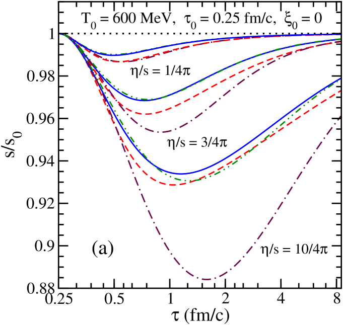
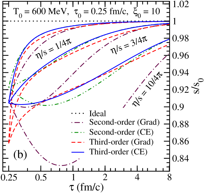
Figure 2: (Color online) Same as Fig. 1 except here we take $T_{0}=600$ MeV.

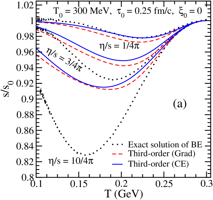
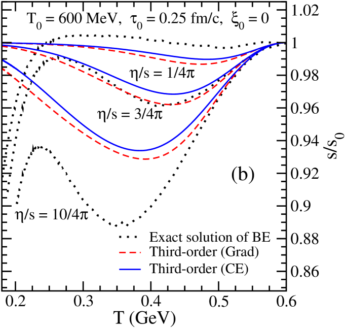
Figure 3: (Color online) Temperature dependence of $s/s_{0}$ obtained using exact solution of the Boltzmann equation (black dotted lines), third-order evolution equations from Grad’s approximation (red dashed lines), and third-order equations from Chapman-Enskog method (blue solid lines) for various $\eta/s$ and for (a): initial temperature $T_{0}=300$ MeV and (b): $T_{0}=600$ MeV, at initial time $\tau_{0}=0.25$ fm/c and isotropic initial pressure configuration $\xi_{0}=0$.

We solve Eqs. (33) and (34) simultaneously assuming two different initial temperatures, $T_{0}=300$ MeV and $T_{0}=600$ MeV, at the initial proper time $\tau_{0}=0.25$ fm/c. The initial pressure configurations are determined by the anisotropy parameter $\xi$ which is related to the average transverse and longitudinal momentum in the local rest frame via the relation $\xi=\frac{1}{2}\langle p_{T}^{2}\rangle/\langle p_{L}^{2}\rangle-1$ Martinez:2010sc . We solve for two different initial pressure configurations: $\xi_{0}=0$ corresponding to an isotropic pressure configuration $\pi_{0}=0$, and $\xi_{0}=10$ corresponding to $\pi_{0}=87$ MeV/fm³ for $T_{0}=300$ MeV and $\pi_{0}=1386$ MeV/fm³ for $T_{0}=600$ MeV. For comparison, we also solve Eqs. (33) and (34) with transport coefficients obtained using the Grad’s 14-moment method El:2009vj .

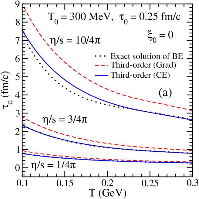
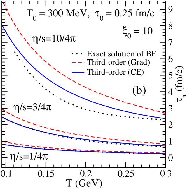
Figure 4: (Color online) Temperature dependence of the shear relaxation time, $\tau_{\pi}$, obtained using exact solution of the Boltzmann equation (black dotted lines), third-order evolution equations from Grad’s approximation (red dashed lines), and third-order equations from Chapman-Enskog method (blue solid lines) for initial temperature $T_{0}=300$ MeV at initial time $\tau_{0}=0.25$ fm/c, various $\eta/s$ and for (a): isotropic initial pressure configuration $\xi_{0}=0$ and (b): anisotropic pressure configuration, $\xi_{0}=10$.

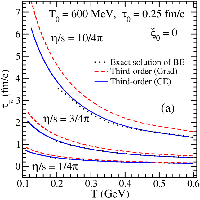
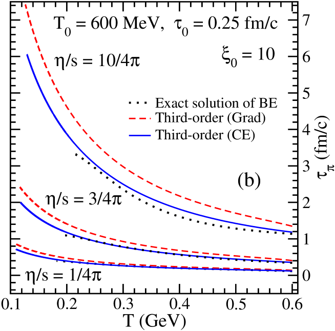
Figure 5: (Color online) Same as Fig. 4 except here we take $T_{0}=600$ MeV.

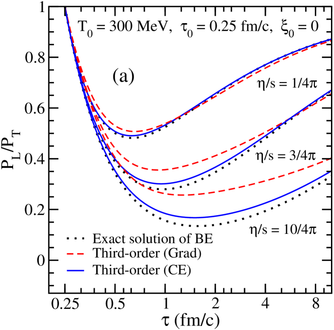
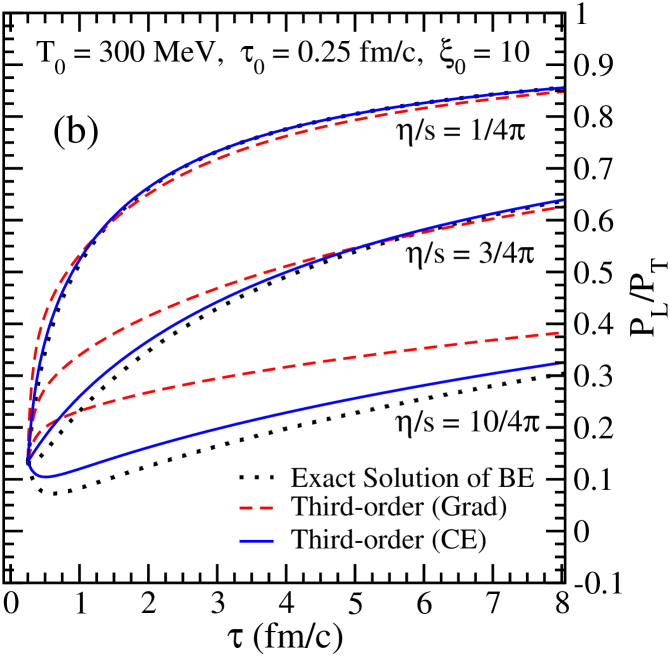
Figure 6: (Color online) Time evolution of $P_{L}/P_{T}$ obtained using exact solution of the Boltzmann equation (black dotted lines), third-order evolution equations from Grad’s approximation (red dashed lines), and third-order equations from Chapman-Enskog method (blue solid lines) for initial temperature $T_{0}=300$ MeV at initial time $\tau_{0}=0.25$ fm/c, various $\eta/s$ and for (a): isotropic initial pressure configuration $\xi_{0}=0$ and (b): anisotropic pressure configuration, $\xi_{0}=10$.

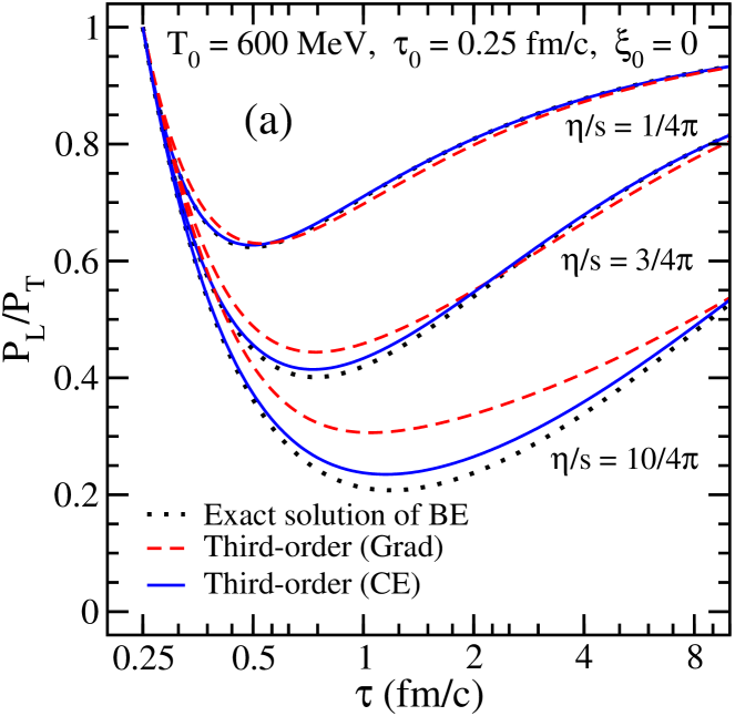
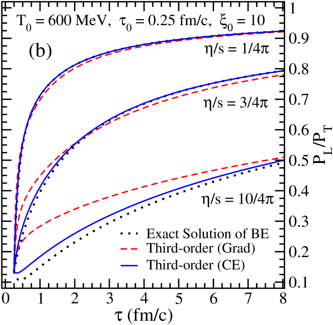
Figure 7: (Color online) Same as Fig. 6 except here we take $T_{0}=600$ MeV.

In Figs. 1 and 2 we show the proper-time evolution of the entropy density scaled by its equilibrium value, $s/s_{0}$, obtained using ideal hydrodynamics (black dotted lines), second-order Grad’s approximation (maroon dashed-dotted lines), second-order Chapman-Enskog (green dashed-dotted-dotted lines), third-order Grad’s approximation (red dashed lines), and third-order Chapman-Enskog method (blue solid lines). Figure 1 shows the case when initial temperature $T_{0}=300$ MeV, while Fig. 2 shows the case that $T_{0}=600$ MeV. In both figures, panels (a) and (b) correspond to isotropic initial pressure configuration $\xi_{0}=0$ and anisotropic pressure configuration $\xi_{0}=10$, respectively, and the initial time $\tau_{0}=0.25$ fm/c.

In the left panels of Figs. 1 and 2, we see that $s/s_{0}$ shows a minimum indicating that the initial and final states of the system are close to equilibrium. In the intermediate stage, viscous evolution leads to significant deviation of the entropy density from its equilibrium value. Moreover, we also observe that for Grad’s method, second-order results are highly sensitive to $\eta/s$ and third-order contribution is very large, especially for large $\eta/s$. On the other hand, Chapman-Enskog method shows less sensitivity to $\eta/s$ and has small third-order contribution indicating faster convergence compared to the Grad’s method. From Figs. 1 and 2, we also observe that the entropy density attains its equilibrium value more rapidly for higher $T_{0}$ indicating that the system equilibrates faster for larger initial temperature. On the other hand, in Fig. 3, we see that both Grad’s method (red dashed lines) and Chapman-Enskog method (blue solid lines) are unable to reproduce the temperature dependence of $s/s_{0}$ obtained using the exact solution of the Boltzmann equation Florkowski:2013lza ; Baym:1984np (black dotted lines) for $T_{0}=300$ MeV and $T_{0}=600$ MeV.

In Figs. 4 and 5 we show the temperature dependence of the shear relaxation time, $\tau_{\pi}$, and in Figs. 6 and 7 we show the proper time evolution of the pressure anisotropy, $P_{L}/P_{T}\equiv(P-\pi)/(P+\pi/2)$. The presented results correspond to exact solution of the Boltzmann equation (black dotted lines), third-order evolution equations from Grad’s approximation (red dashed lines), and third-order equations from Chapman-Enskog method (blue solid lines). Figures 4 and 6 show the case when initial temperature $T_{0}=300$ MeV, while Figs. 5 and 7 show the case that $T_{0}=600$ MeV. In Figs. 4 – 7, panels (a) and (b) correspond to isotropic initial pressure configuration $\xi_{0}=0$ and anisotropic pressure configuration $\xi_{0}=10$, respectively, and the initial time $\tau_{0}=0.25$ fm/c.

From Figs. 4 – 7, we see that results obtained using the Grad’s method always overestimate the shear relaxation time and fails to reproduce the pressure anisotropy obtained by the exact solution of the Boltzmann equation Florkowski:2013lza ; Baym:1984np . On the other hand, the Chapman-Enskog method clearly shows a better agreement with the exact solution of the Boltzmann equation and appreciable differences are observed only for the case of $\eta/s=10/4\pi$. We note that although both methods fail to reproduce the temperature dependence of $s/s_{0}$ obtained using the exact solution of the Boltzmann equation (see Fig. 3), the evolution of pressure anisotropy and shear relaxation time are found to be similar. Therefore we may conclude that the evolution of hydrodynamic quantities are insensitive to small variations in $s/s_{0}$. These results also indicate that the Chapman-Enskog method is better suited than the Grad’s method to capture the microscopic dynamics contained in the Boltzmann equation.

In order to compare our results with a transport model, the parton cascade BAMPS El:2009vj ; Xu:2004mz , we also solve Eqs. (33) and (34) for $T_{0}=500$ MeV at $\tau_{0}=0.4$ fm/c and $\xi_{0}=0$. In Fig. 8, we show the proper time evolution of $P_{L}/P_{T}$ obtained using BAMPS (black dots), third-order evolution equations from Grad’s approximation (red dashed lines), and third-order equations from Chapman-Enskog method (blue solid lines). We see that also in this case the $P_{L}/P_{T}$ obtained using the Chapman-Enskog method show better agreement with BAMPS results compared to Grad’s method. This result confirms our previous observation that Chapman-Enskog method is better adapted than the Grad’s method to capture the microphysics contained in the Boltzmann equation.

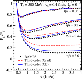
Figure 8: (Color online) Time evolution of $P_{L}/P_{T}$ obtained using BAMPS (black dots), third-order evolution equations from Grad’s approximation (red dashed lines), and third-order equations from Chapman-Enskog method (blue solid lines) for initial temperature $T_{0}=500$ MeV at initial time $\tau_{0}=0.4$ fm/c, isotropic initial pressure configuration $\xi_{0}=0$ and various $\eta/s$.

VI Conclusions and outlook

In this paper, we have employed the iterative solution of the Boltzmann equation in relaxation-time approximation to derive a new expression for the entropy four-current up to third order in gradient expansion. We found that unlike second-order and third-order entropy four-current obtained using Grad’s method, there is a non-vanishing entropy flux in our expression even in the absence of bulk viscosity and dissipative charge current. Having obtained the full set of third-order evolution equations necessary to evolve the shear tensor, we then considered the special case of a transversally homogeneous and longitudinally boost-invariant system. In this particular case the Boltzmann equation in the relaxation-time approximation can be solved exactly Florkowski:2013lza ; Baym:1984np . Using this solution as a benchmark, we computed the entropy density, the shear relaxation time and pressure anisotropy using both the Chapman-Enskog method presented herein and the Grad’s 14-moment method used in Ref. El:2009vj . We also compared the pressure anisotropy obtained using both the Chapman-Enskog method presented herein and the Grad’s method with the results of the parton cascade BAMPS El:2009vj ; Xu:2004mz . We demonstrated that the Chapman-Enskog method is able to reproduce the exact solution of Boltzmann equation as well as the BAMPS results better than the Grad’s method.

As a final remark, we note that the relaxation-time approximation for the collision term in the Boltzmann equation is based on the assumption that the collisions tend to restore the distribution function to its local equilibrium value exponentially. While it is true that the microscopic interactions of the constituent particles are not captured here, it is a reasonably good approximation to describe a system which is close to local thermodynamic equilibrium. Indeed, it was shown that for a purely gluonic system at weak coupling and hadron gas with large momenta, the Boltzmann equation in the relaxation-time approximation is a fairly accurate description Dusling:2009df . Moreover, the experimentally observed and ideal hydrodynamic prediction of $1/\sqrt{m_{T}}$ scaling of the femtoscopic radii was found to be violated by including viscous corrections to the distribution function using Grad’s method Teaney:2003kp . It was shown later that this scaling can be restored by using the form of the non-equilibrium distribution function obtained using the Chapman-Enskog method Bhalerao:2013pza . It has also been demonstrated recently that in contrast to the Grad’s approximation, the renormalization-group method leads to similar expressions for the transport coefficients as given by the Chapman-Enskog method Tsumura:2013uma . Hence we can conclude that the Boltzmann equation in the relaxation-time approximation can be applied quite successfully toward understanding the hydrodynamic behaviour of the strongly interacting matter formed in relativistic heavy-ion collisions.

At this juncture, we would like to clarify that we are using the exact solution of the Boltzmann equation in relaxation-time approximation Florkowski:2013lza ; Baym:1984np as a benchmark to compare different hydrodynamic formulations. We demand that the minimal requirement for a viable conformal hydrodynamic theory is that it should be able to describe the evolution of a viscous medium in this simple case. Moreover, we have demonstrated that the Chapman-Enskog method leads to a fairly good agreement with the BAMPS results El:2009vj ; Xu:2004mz which employs a more realistic collision kernel. Looking forward, it would be interesting to see if the third-order results derived herein could be extended to a system having bulk viscosity and dissipative charge current. Furthermore, since a large bulk viscosity might lead to an early onset of cavitation, it would therefore be instructive to see how the third-order transport coefficients could influence cavitation Jaiswal:2013fc . In addition, from a phenomenological perspective, it would be interesting to determine the impact of the third-order evolution equations in higher-dimensional simulations. We leave these questions for future work.

- (1) U. Heinz and R. Snellings, Ann. Rev. Nucl. Part. Sci. 63, 123 (2013).
- (2) P. Danielewicz and M. Gyulassy, Phys. Rev. D 31, 53 (1985).
- (3) P. Kovtun, D. T. Son and A. O. Starinets, Phys. Rev. Lett. 94, 111601 (2005).
- (4) C. Eckart, Phys. Rev. 58, 267 (1940).
- (5) L.D. Landau and E.M. Lifshitz, Fluid Mechanics (Butterworth-Heinemann, Oxford, 1987).
- (6) H. Grad, Comm. Pure Appl. Math. 2, 331 (1949).
- (7) I. Muller, Z. Phys. 198, 329 (1967).
- (8) W. Israel and J. M. Stewart, Ann. Phys. 118, 341 (1979).
- (9) P. Huovinen and D. Molnar, Phys. Rev. C 79, 014906 (2009).
- (10) S. Chapman and T. G. Cowling, The Mathematical Theory of Non-Uniform Gases, (Cambridge University Press, Cambridge, 1970), 3rd ed.
- (11) A. Jaiswal, Phys. Rev. C 87, 051901 (2013); arXiv:1408.0867 [nucl-th].
- (12) A. Jaiswal, Phys. Rev. C 88, 021903 (2013); Nucl. Phys. A 931, 1205 (2014).
- (13) A. Jaiswal, R. Ryblewski and M. Strickland, Phys. Rev. C 90, 044908 (2014).
- (14) A. Muronga, Phys. Rev. C 69, 034903 (2004)
- (15) G. S. Denicol, T. Koide and D. H. Rischke, Phys. Rev. Lett. 105, 162501 (2010).
- (16) M. A. York and G. D. Moore, Phys. Rev. D 79, 054011 (2009).
- (17) G. S. Denicol, H. Niemi, E. Molnar and D. H. Rischke, Phys. Rev. D 85, 114047 (2012).
- (18) A. Jaiswal, R. S. Bhalerao and S. Pal, Phys. Lett. B 720, 347 (2013); J. Phys. Conf. Ser. 422, 012003 (2013); arXiv:1303.1892 [nucl-th].
- (19) A. Jaiswal, R. S. Bhalerao and S. Pal, Phys. Rev. C 87, 021901(R) (2013).
- (20) R. S. Bhalerao, A. Jaiswal, S. Pal and V. Sreekanth, Phys. Rev. C 88, 044911 (2013).
- (21) R. S. Bhalerao, A. Jaiswal, S. Pal and V. Sreekanth, Phys. Rev. C 89, 054903 (2014).
- (22) M. Martinez and M. Strickland, Nucl. Phys. A 848, 183 (2010).
- (23) W. Florkowski and R. Ryblewski, Phys. Rev. C 83, 034907 (2011).
- (24) M. Martinez, R. Ryblewski and M. Strickland, Phys. Rev. C 85, 064913 (2012).
- (25) W. Florkowski, R. Ryblewski and M. Strickland, Nucl. Phys. A 916, (2013) 249; Phys. Rev. C 88, (2013) 024903.
- (26) D. Bazow, U. W. Heinz and M. Strickland, Phys. Rev. C 90, 054910 (2014).
- (27) A. El, Z. Xu and C. Greiner, Phys. Rev. C 81, 041901 (2010).
- (28) A. Muronga, J. Phys. G 37, 094008 (2010).
- (29) A. Muronga, Acta Phys. Polon. Supp. 7, 197 (2014).
- (30) G. S. Denicol, W. Florkowski, R. Ryblewski and M. Strickland, Phys. Rev. C 90, 044905 (2014).
- (31) W. Florkowski, E. Maksymiuk, R. Ryblewski and M. Strickland, Phys. Rev. C 89, 054908 (2014).
- (32) G. Baym, Phys. Lett. B 138, 18 (1984).
- (33) Z. Xu and C. Greiner, Phys. Rev. C 71, 064901 (2005); 76, 024911 (2007).
- (34) J. L. Anderson and H. R. Witting Physica 74, 466 (1974).
- (35) P. Romatschke, Phys. Rev. D 85, 065012 (2012).
- (36) S.R. de Groot, W.A. van Leeuwen, and Ch.G. van Weert, Relativistic Kinetic Theory — Principles and Applications (North-Holland, Amsterdam, 1980).
- (37) J. D. Bjorken, Phys. Rev. D 27, 140 (1983).
- (38) K. Dusling, G. D. Moore and D. Teaney, Phys. Rev. C 81, 034907 (2010)
- (39) D. Teaney, Phys. Rev. C 68, 034913 (2003)
- (40) K. Tsumura and T. Kunihiro, arXiv:1311.7059 [physics.flu-dyn].