AN INEQUALITY-CONSTRAINED SL/QP METHOD FOR MINIMIZING THE SPECTRAL ABSCISSA

Abstract

We consider a problem in eigenvalue optimization, in particular finding a local minimizer of the spectral abscissa - the value of a parameter that results in the smallest value of the largest real part of the spectrum of a matrix system. This is an important problem for the stabilization of control systems. Many systems require the spectra to lie in the left half plane in order for them to be stable. The optimization problem, however, is difficult to solve because the underlying objective function is nonconvex, nonsmooth, and non-Lipschitz. In addition, local minima tend to correspond to points of non-differentiability and locally non-Lipschitz behavior. We present a sequential linear and quadratic programming algorithm that solves a series of linear or quadratic subproblems formed by linearizing the surfaces corresponding to the largest eigenvalues. We present numerical results comparing the algorithms to the state of the art.

1 Eigenvalue Problem

The problem of interest can be written in the form,

$$\min_{x\in\Re^{n}}f(x)=\min_{x}\alpha(F(x)),$$ (1)

where the spectral abscissa $\alpha$ is defined to be,

$$\alpha(F(x))=\max_{i}\mathfrak{Re}\left(\lambda_{i}(F(x))\right),$$

with $\{\lambda_{i}(F(x))\}$ is the (possibly infinite) spectrum of the matrix $F(x)$ and $F:\Re^{n}\to\Re^{N\times N}$ is two times continuously differentiable. The spectral abscissa corresponds to the largest real part of the eigenvalues of $F(x)$. Recall that the set of matrices with semi-simple eigenvalues is dense in $\Re^{N\times N}$ and $\frac{d\lambda_{i}(F(x))}{dx}$ is continuous with respect to $x$ for all $i$ and all $x$ such that $F(x)$ has only semi-simple eigenpairs, and so $\lambda_{i}(F(x))$ is locally smooth for a.e. $x$.

For instance, in the field of linear output feedback control, $F(x)$ is defined to be,

$$F(x)=A+BXC,$$

where $A$ is the open-loop matrix for the system, $B$ the input matrix and $C$ the output matrix, and $X$ is formed by arranging the components of $x$ into a matrix of the appropriate dimensions.

The optimization problem is difficult to solve for several reasons:

1. It is nonconvex, with possibly many local minimizers and, even arbitrarily close to a local minimizer, the spectral abscissa function typically (but not universally) has negative curvature.

2. It is nonsmooth. As the parameter $x$ changes, each eigenvalue changes as well, usually in a smooth way, however at points where one smooth eigenvalue surface overtakes another one, points of nonsmoothness arise.

3. It is non-Lipschitz. This occurs in the case of a non semi-simple eigenvalue, at which perturbations of the parameter can result in entirely different spectra (for instance, let $x_{c}$ be such that $F(x_{c})$ has a non semi-simple eigenvalue, and there exists a complex conjugage eigen-pair for $x>x_{c}$ and two real pairs for $x<x_{c}$, with the inequalities taken component-wise). Moreover, local minimizers often tend to correspond to these points.

These properties induce a challenging task for optimization algorithms. There are many algorithms suitable for nonconvex smooth or convex nonsmooth optimization problems, but few that are able to solve nonconvex, nonsmooth problems. Furthermore, locally Lipschitz objective functions seem to be universally assumed in the analysis of algorithms (such as local convergence of Newton-like methods, and sufficient descent and bounded steps of proximal-type first order algorithms).

On the other hand, the spectral abscissa is a smooth function almost everywhere (a.e.) in any standard measure of $\Re^{n}$, so the problem is tractable without necessitating the use of sub-gradients, since gradients can be computed at an arbitrary point with probability one. However, local minimizers typically correspond to points of nonsmoothness, and so any algorithm seeking a minimizer of $\alpha(F(x))$ should still take into account that the points to which the sequence of iterates it generates should be attracted to points at which no unique gradient is defined.

We present the graph of a two-dimensional problem in Figure 1. In this example, first given in [19], $F(x)=A+BK$, with,

$$A=\begin{pmatrix}0.1&-0.03&0.2\\ 0.2&0.05&0.01\\ -0.06&0.2&0.07\end{pmatrix},\,\,B=\frac{1}{2}\begin{pmatrix}-1\\ -2\\ 1\end{pmatrix},\,\,K^{T}=\begin{pmatrix}x_{1}\\ x_{2}\\ 1.4\end{pmatrix}$$

Notice that all of the features of $\alpha(F(x))$ we describe above, nonconvexity, nonsmoothness and non-Lipchitz behavior are evident in the figure.

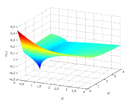
Figure 1: $f(x)$ for a two-dimensional eigenvalue optimization problem.

1.1 Previous work

A number of authors have looked at the problem of achieving matrix stability by minimizing the spectral abscissa [6, 5, 13, 4, 2, 17, 3]. Typically, at each iteration information from a set of gradients is used to generate the next step. There are two primary methods of generating and using the appropriate set of gradients. First, in sampling methods, a set of gradients is generated by sampling around the current point, which serves to approximate the subgradient at a nearby point of nonsmoothness, and a step in the convex hull of the sampled gradients is taken [6, 5]. By contrast, in ”bundle” methods, originally developed for convex nonsmooth optimization [12] build gradient information by mtaintaining historically calculated subgradients during the course of the iterations, and at each point solve cutting-plane underapproximations of the function. In the case of non-convex problems, the analogue of bundle methods is less clear, but various algorithms exist (see, e.g., [8]). Finally we mention a unique contribution that is not comprehensively described by belonging to either of the two categories, and is specifically and algorithm for the context of eigenvalue optimization. In [17] the $\epsilon$ Clarke-subdifferential is approximated by taking the eigenvalues within $\epsilon$ of one with the largest real part and their derivatives with respect to $x$. This resembles our approach in using derivative information from multiple eigenvalue surfaces.

There are a limited number of solvers suitable for eigenvalue optimization problems. In this paper we compare our results to HANSO [18], a code that uses a combination of a BFGS and a gradient sampling search step. BFGS has been shown to exhibit good convergence properties for nonsmooth problems [14]. In particular, we have noticed HANSO tends to interpret points where the objective function surface locally looks like a cusp (i.e., the function is nonsmooth and locally concave in a dense region around the point, the typical situation at a local minimizer of $\alpha(F(X))$), the Hessian approximation’s largest eigenvalue grows without bound. The second order method is eventually drawn to such points, which the gradient sampling procedure [6] refines.

1.2 Contribution

Recall that the spectral abscissa function $\alpha(F(x))$ is smooth almost everywhere. This is because for each eigenvalue, for a.e. $x$, locally there exists a smooth surface $\lambda_{i}(x)$ respect to $x$ that describes how the eigenvalue changes with respect to $x$. For a.e. $x$, $\alpha(F(x))$ corresponds to the surface that is associated with the eigenvalue with the maximal real part. Points where $\alpha(F(x))$ is nonsmooth correspond to two situations: 1) a switch in which eigenvalue corresponds to the maximal real part as $x$ changes, or 2) a splitting of the eigenvalue surface set at a multiple non-semi-simple eigenvalue, in which case the maximal surface can be non-Lipschitz.

The procedures implemented and analyzed thus far only uses the maximal eigenvalue surface, and only after extensively sampling regions with other maximal eigenvalues does it refine its steps relative to the behavior of the function between these regions. Instead, we consider the possibility of explicitly including every one, or at least a large subset, of the eigenvalue surfaces at each point in the calculation of a step with a linearized or quadratic approximation. In the case where nonsmoothness corresponds to changes in which one eigenvalue surface overtakes another one, this should encourage better steps by anticipating in the model where the maximal eigenvalue changes, and as a result taking a step that considers both surfaces and, e.g., moving down a valley in the topography of $\alpha(F(x))$. In the case of points corresponding to a multiple non semi-simple eigenvalue, we introduce memory to include the surface on either side of the point of nonsmoothness, which we expect to decrease the number of iterations needed for the optimization procedure to take steps that decrease the objective function near these non-Lipschitz points.

Thus, in constrast to previous methods, which uses sampled or historical linearizations close to the current iterate to compute a descent step, the algorithm we present uses linearization information of all, or a selected number of the eigenvalue surfaces at the current iterate. We believe that this will allow for larger steps to be taken, resulting in a relatively smaller number of iterations required to reach a local minimizer.

In this paper we include extensive numerical results comparing our algorithm and HANSO. We do not, however, include theoretical convergence analysis. We believe that that for the case where the spectral abscissa function is locally Lipschitz (which would hold if all eigenvalues of $F(x)$ are semi-simple for all $x$), then such a proof would be simple and straightforward by standard arguments. However, in the general case, minimization of non-locally-Lipschitz functions is a very difficult problem with respect to convergence theory. We note that the convergence proof for gradient sampling [6] relies on the local Lipschitz property.

1.3 Notation

We will assume that the eigenvalues are ordered by their real components, with ties broken arbitrarily, i.e.,

$$\mathfrak{Re}(\lambda_{0}(F(x)))\geq\mathfrak{Re}(\lambda_{1}(F(x)))\geq\mathfrak{Re}(\lambda_{2}(F(x)))\geq...$$

note that this ordering is dependent on $x$.

2 SL/QP for Eigenvalue Optimization

In this section we present a sequential quadratic programming (SQP) method, as well as a more simplified Sequential Linear Programming (SLP) method for minimizing the spectral absicssa. The algorithm is a trust-region based method based on the realization that the problem $\min_{x\in\Re^{n}}\alpha(F(x))$ can be rewritten as,

$$\begin{array}[]{rl}\min_{\gamma\in\Re,x\in\Re^{n}}&\gamma,\\ \text{subject to}&\gamma\geq\mathfrak{Re}(\lambda_{i}(F(x)))\text{ for all }i.\end{array}$$ (2)

One key observation to inspire the algorithm is that the number of points at which the objective function $\alpha(F(x))$ in (1) is nonsmooth is of measure zero in the Lebesgue space $\Re^{n}$. This implies that for a.e. $x$, the function $\alpha(F(x))$ is a locally smooth surface. This surface corresponds to the value of $\lambda_{0}(F(x))$ as a function of $x$.

Locally, we can express a linear approximation of the spectral abscissa function as a plane through the point $(x,\alpha(F(x)))$ with the gradient $\nabla_{x}\alpha(F(x))=\nabla_{x}\lambda_{0}(F(x))$, if $\lambda_{0}(F(x))$ is simple. We can calculate both this vector as well as $\nabla^{2}_{xx}\lambda_{i}(F(x))$ by the formulas [10, 15],

$$\nabla_{x}\lambda_{i}(F(x))=\frac{u_{i}^{*}\frac{dF}{dx}v_{i}}{u_{i}^{*}v_{i}},$$ (3)

$$\nabla^{2}_{xx}\lambda_{i}(F(x))=\frac{2u_{i}^{*}\left(\frac{dF}{dx}\right)K_{i}(\lambda_{i}I-F(x))^{\dagger}K_{i}\left(\frac{dF}{dx}\right)v_{i}}{u^{*}_{i}v_{i}},$$ (4)

where $u_{i}$ and $v_{i}$ are the left and right eigenvectors of $F(x)$ corresponding to eigenvalue $i$, $u^{*}$ corresponds to the conjugate of $u$, $\dagger$ is the pseudo-inverse, and $K=I-v_{i}u_{i}^{*}/(u^{*}_{i}v_{i})$.

The Lagrangian function for the problem (2) is defined as,

$$L(\gamma,x)=\gamma-\sum_{i}y_{i}(\gamma-\mathfrak{Re}\left(\lambda_{i}(F(x))\right)),$$ (5)

where $y$ is the vector of Lagrange multipliers.

This naturally suggests the SQP method wherein a sequence of iterations $x_{k+1}=x_{k}+t\Delta x$ is calculated, with $t$ a line-search scalar and $\Delta x$ is determined by solving subproblems of the form,

$$\begin{array}[]{rl}\min_{\Delta x,\Delta\gamma}&\Delta\gamma+\frac{1}{2}\Delta x^{T}H_{k}\Delta x,\\ \text{subject to}&\Delta\gamma+\alpha(F(x_{k}))\geq\mathfrak{Re}(\lambda_{i}(F(x_{k})))+\mathfrak{Re}(\nabla_{x}\lambda_{i}(F(x_{k})))^{T}\Delta x,\forall i,\end{array}$$ (6)

for $\Delta x$ and $\Delta\gamma$, where $H_{k}$ is a Lagrangian Hessian term at $x_{k}$. This resembles the minimax subproblem arising in bundle methods [12], except that the linearizations are defined around a set of eigenvalues of $F(x)$ evaluated at one $x_{k}$. At each iteration we discard $\Delta\gamma$ and compute $\gamma_{k+1}=\alpha(F(x_{k+1}))$ instead and so the iteration procedure behaves like a slack reset in nonlinear programming. To determine the Lagrangian Hessian, we do not use the multipliers from the quadratic programs as estimates for the Lagrangian multipliers. This is because the linearizations are local, and the surfaces they correspond to may disappear from one point to the next (in case of a non-semi-simple eigenvalue between them), and so each constraint may not correspond in any meaningful way to a constraint estimated previously. In the sense of problem (2), the eigenvalues in the set $\operatorname*{Arg\,max}_{i=0,1,...}(\mathfrak{Re}(\lambda_{i}(F(x))))$ are the active constraints. For a.e. $x$ this set comprises of at most two elements, corresponding to a conjugate pair, but in this case the surface corresponding to the real value of the eigenvalue as a function of $x$ is the same for each eigenvalue of the pair. So at the start of each iteration, we set the Lagrange multiplier to have $1$ in the component corresponding to the/an eigenvalue with maximal real part, and $0$ otherwise. Using this multiplier, we calculate the Hessian,

$$H_{k}=\mathfrak{Re}\nabla^{2}_{xx}\lambda_{0}(F(x_{k}))).$$

Note that the Lagrangian function (5) is linear with respect to $\gamma$ and so the Hessian only has blocks corresponding to $x$. At each step of the SQP we need only update $x_{k+1}=x_{k}+\Delta x$. The solution $\Delta\gamma$ is discarded.

There are two primary additional features to the basic procedure we have presented in order to make the method more practically successful. First, recall from Section 1, that the underlying problem is non-convex. This implies that at any local quadratic approximation of an eigenvalue surface, the Hessian could be indefinite or even negative definite. This implies that the approximating quadratic program (6) could be unbounded below. We constrain the problem with a trust-region to prevent this. Since we have linear constraints, we use an infinity norm trust-region, which acts as a ”box” limiting the magnitude of the maximal component of $\Delta x$.

$$\begin{array}[]{rl}\min_{\Delta x,\Delta\gamma}&\Delta\gamma+\frac{1}{2}\Delta x^{T}H_{k}\Delta x,\\ \text{subject to}&\Delta\gamma+\alpha(F(x_{k}))\geq\mathfrak{Re}(\lambda_{i}(F(x_{k})))+\mathfrak{Re}(\nabla_{x}\lambda_{i}(F(x_{k})))^{T}\Delta x,\,\forall i,\\ &||\Delta x||_{\infty}\leq\Delta_{k}.\end{array}$$ (7)

Since the Hessian could be indefinite, the solution $\Delta x$ could be a direction of ascent for the objective function. If the second order information is sufficiently accurate then the step should still decrease the objective function. Otherwise, however, it could be that any point along the line segment $x_{k}+t\Delta x$, $t\in[0,1]$ satisfies $\alpha(F(x_{k}+t\Delta x))>\alpha(F(x_{k}))$. Hence, after computing $\Delta x$ we first test if,

$$\alpha(F(x_{k}+\Delta x))<\alpha(F(x_{k})),$$ (8)

in which case we set $x_{k+1}=x_{k}+\Delta x$ and continue to the next iteration. Otherwise, we test for descent,

$$\mathfrak{Re}(\nabla_{x}\lambda_{i}(F(x_{k})))^{T}\Delta x<0,$$ (9)

and if this does not hold we set $\Delta_{k+1}=\gamma_{1}\Delta_{k}$, where $\gamma_{1}$ is a constant satisfying $\gamma_{1}\in(0,1)$, and resolve the subproblem.

If (9) holds, we follow the mixed trust-region/line-search procedure presented by Gertz [9], in which a backtracking line search reduces the size of the step $t$ until decrease is achieved $(\alpha(F(x_{k}+t\Delta x))<\alpha(F(x_{k})))$, and the next trust-region radius corresponds to $t||\Delta x||$.

$$\Delta_{k+1}=\left\{\begin{array}[]{lr}\gamma_{2}\Delta_{k}&\text{ if }\alpha(F((x_{k}+\Delta x))<\alpha(F(x_{k}))\\ t||\Delta x||&\text{ otherwise},\end{array}\right.$$ (10)

where $\gamma_{2}$ is a constant satisfying $\gamma>1$.

We update the trust-region simply by increasing it if we achieve descent, and decreasing it otherwise. For consistency with convergence theory [7], we would enforce sufficient decrease conditions with respect to predicted (from the quadratic approximation) and actual decrease. However, since lax criteria of acceptance (e.g., with a small constant multiplying the predicted-actual decrease ratio) of the step is practically equivalent to this condition, we proceed as in the line-search criteria for the gradient sampling method [6] to just enforce descent.

In addition, recall that near a non semi-simple eigenvalue, there could be qualitatively different eigenvalue surface combinations on either side of a ”valley”, or $n-1$ dimensional hypersurface in $\Re^{n}$ at which $\nabla\lambda_{i}(F(x))$ is undefined. In order to account for this, we added another feature to the algorithm, after observing a certain phenomenon that was typical with the original SQP algorithm with the trust region but without this additional feature. In many cases, the algorithm jammed near valleys of this kind and would frequently converge onto the valley rather than move down along it. This is because locally, the directional derivative of $\alpha(F(x))$ is steeper towards the valley than perpendicular to it, and, furthermore, it has negative curvature along that direction, so a local approximation that regards only the eigenvalue surfaces at a point on one side of the valley will result in the step of steepest decrease being in this direction. Since the surface on the other side of the valley is not accounted for on the original side, this is not incorporated directly into the subproblem. We illustrate this scenario in Figure 2.

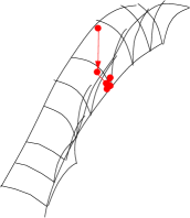
Figure 2: Possible set of iterations of SQP without memory along a surface of $\alpha(F(x))$.

To remedy this, we added ”memory” to the SQP method with a set $\mathcal{M}$. When it occurs that $\alpha(F(x_{k}+\Delta x))>\alpha(F(x_{k}))$, which we expect in the ”jamming” scenario described above, the procedure stores the tuple $\{x_{k}+\Delta x_{k},\mathfrak{Re}(\lambda_{0}(F(x_{k}+\Delta x_{k}))),\nabla_{x}\mathfrak{Re}(\lambda_{0}(F(x_{k}+\Delta x_{k})))\}$ in $\mathcal{M}$. Then, if in a future iteration $l$, the current point $x_{l}$ satisfies $||x_{l}-x^{i}||_{\infty}\leq\Delta_{k}$ for any $i\in\{1,...,|\mathcal{M}|\}$, then we include this linearized surface in the QP subproblem.

$$\begin{array}[]{rl}\min_{\Delta x,\Delta\gamma}&\Delta\gamma+\frac{1}{2}\Delta x^{T}H_{k}\Delta x,\\ \text{subject to}&\Delta\gamma+\alpha(F(x_{k}))\geq\mathfrak{Re}(\lambda_{i}(F(x_{k})))+\mathfrak{Re}(\nabla_{x}\lambda_{i}(F(x_{k})))^{T}\Delta x,\,\forall i\\ &\Delta\gamma+\alpha(F(x_{k}))\geq\mathfrak{Re}(\lambda_{(i)}(F(x^{(i)})))\\ &\qquad\qquad\qquad\qquad+\mathfrak{Re}(\nabla_{x}\lambda_{(i)}(F(x^{(i)})))^{T}(x_{k}+\Delta x-x^{(i)}),\,i\in M_{k}\\ &||\Delta x||_{\infty}\leq\Delta_{k},\end{array}$$ (11)

where $M_{k}\subset\mathcal{M}$ represents the points $x^{(i)}$ satisfying $||x^{(i)}-x_{k}||\leq\Delta_{k}$.

It can be pointed out that this resembles gradient bundle algorithms, which uses gradient information from previous iterations to generate the current step. We acknowledge the resemblance, but point out that in this case historical gradient information is only added in the limited case of a failed trial step, rather than used in each iteration, it is only used when the underlying eigenvalue surfaces change. Local eigenvalue surface approximations, however, are used at each iteration.

Finally, we consider two simplifications of the subproblem. First, we consider dropping the Hessian term, to formulate a sequential linear programming procedure. We note that the lack of a Lipschitz property makes local quadratic convergence difficult to prove for any SQP/Newton type scheme, and so it is quite possible that second derivatives will not reduce the computation time. In addition, with possibly nonconvex subproblems, QP subproblems could result in a series of ascent steps requiring resolving with a smaller trust-region, whereas with LP subproblems, descent is guaranteed for any solution.

We present the SLP version below (12) and summarize the full algorithm as Algorithm 1, for simplicity, and discuss a comparison of the SLP and SQP variant in the numerical results section. Note that we can select a subset of the eigenvalues $N_{k}$ at each iteration $k$ to evaluate and linearize. For small problems, we set $N_{k}=N$ for all $k$ (where, recall that $F(x)\in\Re^{N\times N}$).

$$\begin{array}[]{rl}\min_{\Delta x,\Delta\gamma}&\Delta\gamma,\\ \text{subject to}&\Delta\gamma+\alpha(F(x_{k}))\geq\mathfrak{Re}(\lambda_{i}(F(x_{k})))\\ &\qquad\qquad\qquad\qquad+\mathfrak{Re}(\nabla_{x}\lambda_{i}(F(x_{k})))^{T}\Delta x,\,i\in\{0,...,N_{k}\}\\ &\Delta\gamma+\alpha(F(x_{k}))\geq\mathfrak{Re}(\lambda_{(i)}(F(x^{(i)})))\\ &\qquad\qquad\qquad\qquad+\mathfrak{Re}(\nabla_{x}\lambda_{(i)}(F(x^{(i)})))^{T}(x_{k}+\Delta x-x^{(i)}),\,i\in M_{k}\\ &||\Delta x||_{\infty}\leq\Delta_{k}.\end{array}$$ (12)

The stopping criterion corresponds to the step becoming small, without any new information (memory) being added at the current iteration.

Algorithm 1 SLP Algorithm for Eigenvalue Optimization.

1:Define constants $0<\gamma_{1}<1$, $\gamma_{2}>1$, $\delta_{m}>0$, and $S\in\mathbb{N}$.

2:Determine $N_{0}$. Typically, set $N_{0}=N$, the size of $F(x)$.

3:for $S$ times do

4:     Randomly select starting point $x_{0}$.

5:     Set $\mathcal{M}_{1}=\emptyset$. Set $k=1$.

6:     Calculate initial $\{\lambda_{i}(F(x_{0}))\}$ and $\{\nabla_{x}\lambda_{i}(F(x_{0}))\}$ for $i\in\{0,..,N_{0}\}$.

7:     while ($||\Delta x||>\delta_{m}$ or $\mathcal{M}_{k}\neq\mathcal{M}_{k-1}$) do

8:         Solve (12) for $\Delta x_{k}$.

9:         Calculate $\{\lambda_{i}(F(x_{k}+\Delta x_{k}))\}$ and $\{\nabla_{x}\lambda_{i}(F(x_{k}+\Delta x_{k}))\}$ for $i\in\{0,..,N_{k}\}$

10:         if $\alpha(F(x_{k}+\Delta x_{k}))<\alpha(F(x_{k}))$ then

11:              Set $x_{k+1}\leftarrow x_{k}$

12:              Set $\Delta_{k+1}\leftarrow\gamma\Delta_{k}$.

13:         else

14:              Store $\{x_{k}+\Delta x_{k},\mathfrak{Re}(\lambda_{0}(F(x_{k}+\Delta x_{k}))),\nabla_{x}\mathfrak{Re}(\lambda_{0}(F(x_{k}+\Delta x_{k})))\}$

15:                    in $\mathcal{M}_{k+1}$.

16:              Find $t$ such that $\alpha(F(x_{k}+t\Delta x_{k}))<\alpha(F(x_{k}))$.

17:              Set $x_{k+1}\leftarrow x_{k}+t\Delta x_{k}$.

18:              Set $\Delta_{k+1}\leftarrow t||\Delta x_{k}||$.

19:         end if

20:         Set $k\leftarrow k+1$.

21:         Determine $N_{k}$. Typically, set $N_{k}=N$, the size of $F(x)$.

22:         Calculate all $\{\lambda_{i}(F(x_{k}))\}$ and $\{\nabla_{x}\lambda_{i}(F(x_{k}))\}$ for $i\in\{0,..,N_{0}\}$.

23:     end while

24:     Add the last point $(x_{f},\alpha(F(x_{f})))$ to $\mathcal{F}$.

25:end forreturn $\{x_{f},\alpha(F(x_{f}))\}$ corresponding to the lowest value of $\alpha(F(x_{f}))$ in $\mathcal{F}$.

In the case of large scale problems, we reduce $N_{k}$ in order to minimize eigenvalue computation time. For large $N$ we use iterative procedures to compute a subset of the eigenvalues corresponding to those farthest to the right in the complex plane. For example, want to calculate all eigenvalues in the right half plane relative to a certain minimal value of some desired $\bar{\lambda}_{c}$. The set $N_{k}$ of eigenvalues we consider may change each iteration. We can choose to either determine $\bar{\lambda}_{c}$ or $N_{k}$ and calculate the appropriate subset of the spectrum. If we decide to select the subset based on a heuristic choice for $N_{k}$, its value should be greater than or equal to the number of active (maximal) eigenvalues, otherwise the choice depends on how many surfaces we want to keep track of, locally. In our implementation we use $2n$. Note that this is the number of sample points to use in a gradient sampling method [6]

3 Numerical Results for Linear Eigenvalue Problems

We compare SLP/SQP to HANSO on a set of linear control problems arising from COMPlib [11]. COMPlib contains a set of linear control matrices, of which we take three for the system $F(x)=A+BXC$. Out of 124 examples, we picked 99 problems with the number of rows (and columns) of $A$ was less than or equal to 50. We found that for both HANSO and SLP/SQP, even for the large-scale variant, many of the problems in the complement of this set took far long to solve to realistically perform numerical comparisons.

For all solvers, we used a stopping tolerance of 1e-6 (indicating that the algorithms stopped when the (inf) norm of the step was smaller than 1e-4). The SL/QP algorithms were coded in MATLAB, with all tests run using MATLAB version 2013a. All tests were performed on an Intel Core 2.2 GHz $\times 8$ running Ubuntu 14.04. For all algorithms we use the same procedure of using ten random starting points as provided by default with HANSO, specifically initializing a point by a normal distribution centered at zero, and then picking the best solution (the one with the lowest objective value) of ten runs. All of the code used for the experiments in this and the next section is available at [1].

We list the parameter and initial values we use in our implementations of SL/QP in Table 1 $0<\gamma_{1}<1$, $\gamma_{2}>1$, $\Delta_{m}>0$, $\delta_{m}>0$, and $S\in\mathbb{N}$. We denote $k_{\text{max}}$ the maximum number of iterations, $LSk_{\text{max}}$ the maximum number of line-search steps, and $\eta$ the backtracking contraction parameter.

Table 1: Control parameters and initial values required by algorithm 1

Parameter	Value	Parameter	Value	Parameter	Value
$\gamma_{1}$	0.1	$S$	10	$k_{\text{max}}$	20
$\gamma_{2}$	2.0	$N_{0}$	$N$	$LSk_{\text{max}}$	20
$\delta_{m}$	1.0e-r	$\Delta_{0}$	1.0	$\eta$	0.5

HANSO was used with its default parameters, including normtol$=$1e-4, evaldist$=$1e-4, and maxit$=$1000.

For these comparisons, we compare both the time of execution as well as the value of the final solution. We summarize the results below in Table 2. If an algorithm returns an error rather than converging, we indicate that as being the worse performer (for no problem did both SLP and a variation of HANSO fail to converge). Note that gradient sampling provides a guarantee of global convergence in the case of the objective being local Lipschitz, however there are no theoretical guarantees for any algorithm without this condition.

Since the problems are all nonconvex, it is difficult to make a straightforward comparison since each run could result in a different local minimizer, and thus we perform a large number of runs for each problem to obtain a global picture. Since for all of the algorithms we sample ten random starting points from a uniformly normal distribution, in the long run, since the algorithms are all purely local in nature (i.e., encouraging convergence to a local minimizer from arbitrary starting points, rather than a global minimizer), a global picture of which algorithm performs more reliably in obtaining a local minimizer can be understood as one for which a) convergence from arbitrary starting points is more likely and b) possibly includes general features that encourages a globally lower objective value. In the results we report the median, minimum, and maximum number of problems for which SLP outperforms HANSO from a set of 50 runs of every small problem.

In general, for most problems, SLP finds a lower minimum than HANSO. It appears to be faster than HANSO with gradient sampling, and slower than BFGS alone. Interestingly, gradient sampling does not, on average, tend to improve the performance of HANSO vis-a-vis SLP.

In the interest of enforcing stability, for SLP, for one run there were 74 problems where the final spectral abscissa (median of 50 runs) was less than zero, as compared to 63 for HANSO with gradient bundle and 59 for HANSO without.

Table 2: Number of times SLP outperformed HANSO out of 99 small problems. Minimum (median) and maximum out of 50 runs. The value for each algorithm is the best out of 10 random starting points for each run and each problem. The time is the total clock time taken to run the algorithm for all of these random starting points.

	in value	in time
HANSO	68 (78) 85	85 (90) 93
HANSO without gradient sampling	67 (78) 85	4 (8) 12

We also performed a comparison of SLP versus SQP on the test problems. The results, in Table 3 indicate that SLP tends to be slightly more reliable and faster. Overall, there is little difference in the performance, however.

Table 3: Performance of SLP as compared to SQP (out of 99 problems, minimum (median) and maximum of 50 runs). The value for each algorithm is the best out of 10 random starting points for each run and each problem. The time is the total clock time taken to run the algorithm for all of these random starting points. (Notice that the sum of the best in value column is not (and is not very close to) $99$, this is because for some problems the result was exactly equal)

Algorithm	best in value	best in time
SLP	41 (51) 61	49 (58) 66
SQP	35 (46) 54	33 (42) 50

Table LABEL:tab.bigtable lists all of the problems, times and values for SLP and the two variations of HANSO. NaN indicates that the solver did not converge for the problem, with either non-convergence or an error indicated. We can see that when there are differences in final value, that the differences are typically relatively substantial. Indeed, note that, in general, it clearly appears that differences in value must correspond to either different local minimizers or failure to converge, rather than a slightly more precise solution.

Table 4: Results for SLP, HANSO, and HANSO without gradient sampling for 99 small COMPleib problems. Value is the best out of 10 runs with random starting points. Time is the total time taken to perform the 10 runs.

Prob	$N$	$n$	t SLP	t HANSO	t H no GS	Value SLP	V HANSO	V H no GS
1	5	9	4.85e-01	8.50e-01	1.35e+01	-1.33e-01	-4.99e-01	-2.05e-01
2	5	9	6.83e-01	8.44e-01	1.33e+01	-3.23e-01	-4.14e-01	-8.81e-02
3	5	8	1.08e+00	8.89e-01	6.96e-01	-1.39e+00	-9.93e-01	-1.35e-01
4	4	2	2.28e-01	3.40e-01	6.73e-02	-5.00e-02	-5.00e-02	-5.00e-02
5	4	4	4.36e-01	6.30e-01	6.37e+00	-8.99e-01	9.66e-01	9.94e-01
6	7	8	7.80e-01	5.20e-01	1.34e+01	-6.46e-01	-7.53e-01	-2.17e-01
7	9	2	3.53e-01	3.07e-01	2.16e-01	-3.62e-02	-3.34e-02	-3.09e-02
8	9	5	7.09e-01	1.08e+00	8.41e+00	-2.50e-01	-3.74e-01	3.36e-02
9	10	20	6.45e-01	9.61e-01	1.41e+01	-2.96e-01	-1.09e-01	-3.04e-02
11	5	8	1.17e+00	1.33e+00	9.39e+00	-8.76e+00	-2.57e+00	-1.17e+00
12	4	12	6.10e-01	8.98e-01	1.23e+01	-2.63e-01	-1.07e-01	-9.38e-02
13	28	12	5.70e-01	9.11e-01	7.00e-01	1.44e-01	1.33e-01	1.42e-01
14	40	12	8.74e-01	9.45e-01	2.24e+01	3.32e-02	1.92e-01	2.22e-01
15	4	6	5.24e-01	9.77e-01	7.56e+00	-4.91e-01	-3.85e-01	-1.46e-01
16	4	8	1.17e+00	1.10e+00	9.50e+00	-7.88e-01	-4.84e-01	-1.68e-01
17	4	2	3.59e-01	5.90e-01	5.42e+00	-9.35e-01	-1.13e+00	-8.92e-01
18	10	4	NaN	3.33e-01	7.89e+00	NaN	1.89e+00	8.89e-01
19	4	2	4.70e-01	2.85e-01	5.48e+00	-2.39e-01	-6.27e-02	-1.49e-01
20	4	4	3.86e-01	3.60e-01	6.52e+00	-7.03e-01	-1.66e-01	-6.26e-01
21	8	24	5.70e-01	1.02e+00	1.88e+01	-2.87e-02	-6.76e-02	1.49e-01
22	8	24	1.72e+00	1.46e+00	1.93e+01	-2.43e-01	-1.08e-01	5.47e-02
23	8	8	1.09e+00	8.30e-01	9.80e+00	-1.60e-02	-6.33e-02	1.76e-01
24	20	24	5.34e-01	1.76e+00	8.18e-01	-5.00e-03	-5.00e-03	3.93e-02
25	20	24	7.49e-01	1.37e+00	4.65e+00	-5.00e-03	-5.00e-03	2.04e-02
26	30	15	1.18e+00	1.41e+00	4.69e-01	5.53e+00	9.36e+00	9.79e+00
27	21	9	6.06e-01	8.94e-01	2.02e+01	-3.82e-01	-4.71e-01	1.98e-01
28	24	18	3.99e-01	2.68e+00	2.78e+01	-6.22e-01	-1.59e+00	2.36e+00
29	4	6	5.62e-01	1.20e+00	9.52e+00	6.89e-02	-2.57e+00	-1.84e+00
30	4	4	5.05e-01	4.25e-01	6.84e+00	-2.11e+00	-1.03e+00	-1.11e+00
31	12	3	7.48e-01	4.52e-01	7.14e+00	-2.07e-02	-2.07e-02	-2.07e-02
32	8	1	2.27e-01	2.28e-01	5.74e+00	7.12e-01	6.63e-01	8.66e-01
33	8	16	8.75e-01	1.22e+00	2.02e+01	-7.99e-01	-7.75e-01	-3.93e-01
34	3	4	1.67e+00	9.95e-01	6.31e+00	-8.52e+00	-1.29e+01	4.49e-01
35	6	16	1.63e+00	1.17e+00	1.47e+01	-4.48e+00	-2.36e+00	-3.81e-01
36	6	24	1.00e+00	1.37e+00	1.87e+01	-1.85e+01	-2.21e+00	-1.02e+00
37	4	4	7.60e-01	9.75e-01	6.57e+00	-2.16e+00	-1.29e+00	8.93e-01
38	10	4	6.79e-01	5.70e-01	7.75e+00	-7.06e-01	-7.11e-01	1.17e-01
39	12	4	3.02e-01	5.91e-01	8.06e+00	-2.16e-01	-2.16e-01	-2.16e-01
40	10	12	4.15e-01	4.15e-01	1.47e+01	-1.71e-01	-4.36e-01	-5.23e-01
41	10	12	5.06e-01	6.07e-01	1.76e+01	-1.56e+00	-1.47e+00	-6.70e-01
42	10	12	4.79e-01	5.52e-01	1.96e+01	-1.10e+00	-4.29e+00	-7.86e-01
44	11	9	9.85e-01	1.36e+00	7.19e-01	-3.62e-03	-6.58e-03	-3.22e-03
46	4	6	8.57e-01	6.83e-01	8.08e+00	-2.65e-02	-3.13e-02	-2.34e-02
47	8	4	7.63e-01	1.11e+00	7.40e+00	1.78e+01	-1.49e+01	-1.17e+01
48	21	110	9.76e-01	1.94e+01	7.22e-01	1.03e+00	1.13e+00	1.22e+00
49	20	20	6.65e-01	1.17e+00	2.94e+01	-9.28e-02	-1.03e-01	-1.12e-01
51	10	1	2.07e-01	2.79e-01	6.22e+00	-1.39e-01	-1.15e-01	-1.23e-01
52	10	1	3.15e-01	2.86e-01	6.16e+00	-1.48e-01	-1.48e-01	-1.13e-01
53	10	1	2.22e-01	2.65e-01	6.22e+00	-9.56e-02	-1.09e-01	-9.84e-02
54	20	1	1.45e+00	5.37e-01	1.10e+01	-8.52e-02	-8.52e-02	-2.02e-02
55	40	1	3.15e+00	1.65e+00	9.88e-01	-4.02e-05	-4.02e-05	-4.01e-05
57	5	3	1.85e-01	1.15e+00	5.95e+00	-5.72e-07	-1.33e-06	-7.57e-07
58	7	8	1.30e+00	1.21e+00	9.94e+00	-6.83e-02	-2.25e-02	9.38e-03
59	7	6	4.32e-01	6.10e-01	NaN	-1.00e-05	-1.00e-05	NaN
60	7	6	6.10e-01	5.95e-01	7.90e+00	3.88e-02	2.91e-03	1.21e-01
61	7	6	5.91e-01	3.67e-01	8.37e+00	-2.11e+00	-1.90e+00	-1.21e+00
64	3	2	2.52e-01	4.42e-01	1.32e+00	1.45e+00	1.48e+00	2.84e+00
65	2	1	5.19e-01	6.89e-01	4.75e+00	-1.00e+00	-1.00e+00	-9.60e-01
66	4	1	NaN	3.47e-01	2.17e-01	NaN	2.18e+00	2.14e+00
67	4	6	7.93e-01	3.87e-01	7.50e+00	-1.31e+00	-6.17e-01	-3.46e-01
68	7	2	9.79e-01	2.91e-01	6.03e+00	1.09e-02	3.36e-01	5.39e-02
69	9	4	4.48e-01	3.56e-01	7.49e+00	6.76e-01	1.91e+00	1.75e+00
70	9	4	5.97e-01	6.35e-01	7.47e+00	1.75e-01	2.49e+00	1.80e+00
71	3	4	1.12e+00	1.12e+00	6.34e+00	-3.81e+00	-1.56e+00	-7.92e-01
72	5	6	1.83e+00	1.01e+00	7.72e+00	-2.92e+00	1.25e-01	5.67e-01
73	8	9	3.06e-01	5.78e-01	1.07e+01	1.33e+00	2.85e+00	1.25e+00
74	16	15	1.01e+00	7.50e-01	1.58e+01	-9.38e-01	-8.88e-01	-9.14e-01
75	6	4	6.04e-01	4.13e-01	6.87e+00	2.04e-01	4.50e-01	6.32e-01
76	6	4	6.07e-01	6.17e-01	6.96e+00	-1.63e+00	6.41e-02	3.97e+00
77	6	4	2.24e-01	6.94e-01	7.01e+00	1.82e+00	-1.64e-01	2.60e+00
78	3	4	8.93e-01	5.62e-01	6.26e+00	-2.29e+00	-4.09e+00	-1.35e+00
79	8	16	2.13e+00	2.08e+00	1.29e+01	-8.31e-03	-3.44e-02	-3.32e-03
80	3	2	5.73e-01	4.53e-01	5.35e+00	-3.26e-01	-4.45e-01	-5.54e-01
91	5	6	6.89e-01	5.08e-01	7.65e+00	-1.31e+00	-2.37e+00	-7.94e-01
92	5	6	8.00e-01	7.50e-01	7.20e+00	-8.88e+00	-2.92e+00	-2.87e+00
93	5	8	5.55e-01	8.38e-01	9.61e+00	-1.38e+00	-8.79e-01	-1.25e+00
94	5	8	8.42e-01	1.11e+00	1.26e+01	-6.12e+00	-7.87e+00	-5.91e+00
95	5	8	8.91e-01	1.21e+00	1.18e+01	-2.38e+00	-2.22e+00	-1.43e+00
96	5	8	6.57e-01	7.67e-01	9.44e+00	-5.38e+00	-4.99e+00	-1.94e+00
97	5	8	1.74e+00	6.35e-01	9.43e+00	-1.41e+00	-8.03e-01	-7.87e-01
98	5	8	5.12e-01	6.16e-01	9.51e+00	-3.33e+00	-9.37e+00	-2.85e+00
99	5	4	7.45e-01	9.34e-01	6.62e+00	-8.50e-02	-2.06e-01	-1.19e-01
100	20	2	1.32e+00	8.71e-01	5.95e-01	-8.90e-03	-9.19e-03	-8.08e-03
106	6	8	5.14e-01	7.57e-01	9.92e+00	-4.53e-02	-7.45e-02	-5.13e-02
107	5	3	1.71e+00	8.67e-01	4.14e+00	-8.33e-04	9.42e-06	6.46e-03
108	10	4	1.63e+00	9.84e-01	7.81e+00	-5.63e-01	-6.02e-01	-1.46e-01
109	40	4	9.68e-01	1.94e+00	3.93e+01	-5.13e-03	-5.40e-03	-4.98e-03
110	40	4	1.17e+00	2.85e+00	1.76e+00	-5.12e-03	-5.53e-03	-5.00e-03
114	48	1	4.43e+00	1.25e+01	5.27e+01	-2.64e-01	-2.66e-01	-2.84e-01
115	9	4	6.30e-01	7.74e-01	7.62e+00	-1.18e-02	-8.45e-03	1.13e-01
116	10	6	3.01e-01	2.03e-01	8.58e+00	4.80e-02	-1.43e-03	1.81e-02
117	11	16	6.07e-01	1.08e+00	1.69e+01	5.21e-01	6.97e-01	8.40e-01
118	9	4	7.13e-01	5.06e-01	7.58e+00	-1.52e-02	-3.33e-03	1.42e-03
119	7	15	4.50e-01	1.04e+00	1.41e-01	3.64e-01	2.48e-01	3.61e-01
120	5	9	4.04e-01	3.77e-01	1.00e+01	2.45e-01	3.36e-01	6.90e-01
121	5	6	7.38e-01	6.77e-01	7.74e+00	-4.56e-02	-3.06e-01	-8.28e-04
122	9	16	1.74e+00	1.18e+00	1.49e+01	3.98e-04	-2.59e-03	5.18e-01
123	6	9	4.71e-01	8.40e-01	1.03e+01	-3.13e-02	-2.05e-02	1.76e-02
124	6	8	5.03e-01	5.10e-01	9.56e+00	1.73e+00	1.37e+00	7.70e-02

4 Nonlinear Eigenvalue Problems

In this section we consider time-delay systems of the form,

$$v^{\prime}(t)=\sum_{j=0}^{m}A_{j}(x)v(t-\tau_{j}).$$

In this case, we have a nonlinear eigenvalue problem. To solve for the eigenvalues, we find the solutions $\lambda(x)$ of,

$$\det(\Lambda(\lambda;x))=0,$$

with,

$$\Lambda(\lambda;x)=\lambda I-A_{0}(x)-\sum_{j=1}^{m}A_{j}(x)e^{-\lambda\tau_{j}}.$$

The number of eigenvalues in this case is generally infinite, but within any right half-plane the number of eigenvalues is finite [16]. In the numerical experiments, we find all of those which are to the right of $r=-1/\tau_{m}$, where $\tau_{m}$ is the maximum of the delays. If none are found, we repeatedly double $r$ until at least one eigenvalue appears.

It can be shown that, in the case where each $A_{i}(x)$ depends smoothly on $x$ and where the eigenvalue has multiplicity 1, the derivative of the surface corresponding to each eigenvalue $\lambda_{i}$ is equal to [16],

$$\nabla_{x}\lambda_{i}=\frac{u^{*}_{i}\left(\frac{\partial A_{0}}{\partial x}+\sum_{j=1}^{m}\frac{\partial A_{j}}{\partial x}e^{-\lambda_{i}\tau_{j}}\right)v_{i}}{u^{*}_{i}\left(I+\sum_{j=1}^{m}\tau_{j}e^{-\lambda\tau_{j}}A_{j}\right)v_{i}}.$$

Note that the term in the numerator, $\frac{\partial A_{0}}{\partial x}+\sum_{j=1}^{m}\frac{\partial A_{j}}{\partial x}e^{-\lambda_{i}\tau_{j}}$ corresponds to $\nabla_{x}F(x)$, and so we can use the same formula for the second derivative, (4) as in the linear case, with $F(x)$ replaced by $F(x,\lambda)=A_{0}(x)+\sum_{j=1}^{m}A_{j}(x)e^{-\lambda\tau_{j}}$.

Alternatively, second-derivatives may be calculated explicitly. Specifically,

$$\begin{array}[]{l}\nabla^{2}_{xx}\lambda_{i}(x)=-\frac{u_{i}^{*}(\nabla^{2}_{x\lambda}\Lambda(\lambda_{i},x)\otimes\nabla_{x}\lambda_{i}+\nabla^{2}_{xx}\Lambda(\lambda_{i},x)+\nabla^{2}_{\lambda\lambda}\Lambda(\lambda_{i},x)\otimes(\nabla_{x}\lambda_{i})\otimes(\nabla_{x}\lambda_{i}))v_{i}}{u_{i}^{*}\nabla_{\lambda}\Lambda(\lambda_{i},x)v_{i}}\\ \qquad+\frac{u_{i}^{*}(2\nabla_{x}\Lambda(\lambda_{i},x)+2\nabla_{\lambda}\Lambda(\lambda_{i},x)\otimes\nabla_{x}\lambda_{i})\nabla_{x}v_{i}}{u_{i}^{*}\nabla_{\lambda}\Lambda(\lambda_{i},x)v_{i}},\end{array}$$

where $\nabla_{x}v_{i}$ can be calculated (along with $\nabla_{x}\lambda_{i}$) by,

$$\begin{pmatrix}\Lambda(\lambda_{i},x)&\nabla_{\lambda}\Lambda(\lambda_{i},x)\\ 2v_{i}^{*}&0\end{pmatrix}\begin{pmatrix}\nabla_{x}v_{i}\\ \nabla_{x}\lambda_{i}\end{pmatrix}=\begin{pmatrix}\nabla_{x}v_{i}\\ 0\end{pmatrix},$$

where the second set of equations comes from differentiating $v_{i}^{*}v_{i}=1$.

We compare the performance of 500 trials of SLP and HANSO with and without gradient sampling for two time-delay systems described in [20].

The first example is a third-order feedback controller system of the form,

$$v^{\prime}(t)=Av(t)+B(x)v(t-5),$$

with $A$ and $B(x)$ defined to be,

$$A=\begin{pmatrix}-0.08&-0.03&0.2\\ 0.2&-0.04&-0.005\\ -0.06&-0.2&-0.07\end{pmatrix}$$

and

$$B(x)=\begin{pmatrix}-0.1\\ -0.2\\ 0.1\end{pmatrix}\begin{pmatrix}x_{1}&x_{2}&x_{3}\end{pmatrix}.$$

We present the results below in Table LABEL:tablenonlin1. In this case, statistically, SLP finds no lower or higher minimizer than HANSO with or without gradient sampling. However, it almost always finds it in less time. In this case, SLP appears to also perform similarly in terms of finding the lowest minimizer as SQP, but now takes less time. We also include the mean and standard deviation of the values and times in Table LABEL:tablenonlin1b. One can consider the true mean time of execution and value at the final solution as a distribution dependent on the initial starting point with unknown form for each algorithm. Therefore, we can take a sample difference of means test to compare the performance. If we take a Student t-test for the difference in means for the times, then even for $0.0001$ significance, the difference in both mean times and values is significant between SLP and HANSO (both with and without gradient sampling).

	in value	in time
HANSO	250	500
HANSO without gradient sampling	257	447
SQP	227	344

	value	time
HANSO	-0.074 (0.036)	177 (30.3)
HANSO without gradient sampling	-0.069 (0.036)	6.1 (2.7)
SLP	-0.081 (0.053)	4.6 (1.1)
SQP	-0.088 (0.055)	5.3 (1.6)

The next example is given below,

$$\begin{array}[]{l}T_{h}\dot{x}_{h}(t)=-x_{h}(t-\eta_{h})+K_{b}x_{a}(t-\tau_{b})+K_{u}x_{h,set}(t-\tau_{u}),\\ T_{a}\dot{x}_{a}(t)=-x_{a}(t)+x_{c}(t-\tau_{e})+K_{a}(x_{h}(t)-\frac{1+q}{2}x_{a}(t)-\frac{1-q}{2}x_{c}(t-\tau_{e})),\\ T_{d}\dot{x}_{d}(t)=-x_{d}(t)+K_{d}x_{a}(t-\tau_{d}),\\ T_{c}\dot{x}_{c}(t)=-x_{c}(t-\eta_{c})+K_{c}x_{d}(t-\tau_{c}),\\ \dot{x}_{e}(t)=-x_{c}(t)+x_{c,set}(t),\end{array}$$

with,

$$x_{h,set}(t)=\begin{pmatrix}K_{1}&K_{2}&K_{3}&K_{4}&K_{5}\end{pmatrix}\begin{pmatrix}x_{h}(t)&x_{a}(t)&x_{d}(t)&x_{c}(t)&x_{e}(t)\end{pmatrix}^{T}.$$

The results, which are qualitatively similar as in the first example, are given in Tables LABEL:tablenonlin2 and LABEL:tablenonlin2b.

	in value	in time
HANSO	268	500
HANSO without gradient sampling	283	466

	value	time
HANSO	-0.077 (0.0052)	2,200 (6400)
HANSO without gradient sampling	-0.067 (0.0054)	69.0 (28)
SLP	-0.083 (0.0062)	83.5 (140)
SQP	-0.088 (0.0103)	75.5 (76)

5 Conclusion

In this paper we studied the eigenvalue optimization problem of minimizing the spectral abscissa, the maximum real eigenvalue part. This problem is important for designing stabilizing controllers, such as in LTI and time-delay models. We presented an algorithm that incorporated linear and quadratic models of eigenvalue surfaces corresponding to different eigenvalues in a sequential linear and sequential quadratic programming framework. We expected this to produce a faster and possibly more reliable algorithm for finding minima of the spectral abscissa, since the model is capable of approximating the spectral abscissa surface past points of nonsmoothness.

Our numerical results for both linear and nonlinear problems borne out our expectation, and we find that, in particular, the sequential linear variant of the algorithm tends to, in general, outperform the most comparable competitor, HANSO. For linear problems, it is faster and more reliable than HANSO with gradient sampling, and more reliable but slower than HANSO without gradient sampling. For nonlinear problems, SLP is faster than and at least equally as reliable as both HANSO and HANSO without gradient sampling.

In future research we intend to study the pseudospectral abscissa, which is a locally Lipschitz function, and hence more readily amenable to theoretical convergence analysis. In addition, researh can include testing these algorithms on interesting large-scale delay and control applications.

6 Acknowledgements

This research was supported by Research Council KUL: PFV/10/002 Optimization in Engineering Center OPTEC, GOA/10/09 MaNet, Belgian Federal Science Policy Office: IUAP P7 (DYSCO, Dynamical systems, control and optimization, 2012-2017); ERC ST HIGHWIND (259 166). V. Kungurtsev was also supported by the European social fund within the framework of realizing the project “Support of inter-sectoral mobility and quality enhancement of research teams at the Czech Technical University in Prague”, CZ.1.07/2.3.00/30.0034.

References

- [1] Slp and sqp code and full compleib and nonlinear experiments. http://twr.cs.kuleuven.be/research/software/delay-control/slp/.
- [2] P. Apkarian, D. Noll, and O. Prot. A trust region spectral bundle method for nonconvex eigenvalue optimization. SIAM Journal on Optimization, 19(1):281–306, 2008.
- [3] J. Burke, A. Lewis, and M. Overton. Optimizing matrix stability. Proceedings of the American Mathematical Society, 129(6):1635–1642, 2001.
- [4] J. V. Burke, D. Henrion, A. S. Lewis, and M. L. Overton. Stabilization via nonsmooth, nonconvex optimization. Automatic Control, IEEE Transactions on, 51(11):1760–1769, 2006.
- [5] J. V. Burke, A. S. Lewis, and M. L. Overton. Two numerical methods for optimizing matrix stability. Linear Algebra and its Applications, 351:117–145, 2002.
- [6] J. V. Burke, A. S. Lewis, and M. L. Overton. A robust gradient sampling algorithm for nonsmooth, nonconvex optimization. SIAM Journal on Optimization, 15(3):751–779, 2005.
- [7] A. R. Conn, N. I. Gould, and P. L. Toint. Trust region methods, volume 1. Siam, 2000.
- [8] A. Fuduli, M. Gaudioso, and G. Giallombardo. Minimizing nonconvex nonsmooth functions via cutting planes and proximity control. SIAM Journal on Optimization, 14(3):743–756, 2004.
- [9] E. M. Gertz et al. Combination trust-region line-search methods for unconstrained optimization. PhD thesis, University of California, San Diego, 1999.
- [10] P. Lancaster. On eigenvalues of matrices dependent on a parameter. Numerische Mathematik, 6(1):377–387, 1964.
- [11] F. Leibfritz. Compleib: Constrained matrix optimization problem library, 2006. URL http://www. complib. de, 2010.
- [12] C. Lemaréchal. Chapter vii nondifferentiable optimization. Handbooks in Operations Research and Management Science, 1:529–572, 1989.
- [13] A. S. Lewis and M. L. Overton. Eigenvalue optimization. Acta numerica, 5:149–190, 1996.
- [14] A. S. Lewis and M. L. Overton. Nonsmooth optimization via quasi-newton methods. Mathematical Programming, 141(1-2):135–163, 2013.
- [15] J. R. Magnus. On differentiating eigenvalues and eigenvectors. Econometric Theory, 1(2):pp. 179–191, 1985.
- [16] W. Michiels and S.-I. Niculescu. Stability and stabilization of time-delay systems: an eigenvalue-based approach, volume 12. Siam, 2007.
- [17] D. Noll and P. Apkarian. Spectral bundle methods for non-convex maximum eigenvalue functions: first-order methods. Mathematical programming, 104(2-3):701–727, 2005.
- [18] M. Overton. Hanso: a hybrid algorithm for nonsmooth optimization. Available from cs.nyu.edu/overton/software/hanso, 2009.
- [19] J. Vanbiervliet, B. Vandereycken, W. Michiels, S. Vandewalle, and M. Diehl. The smoothed spectral abscissa for robust stability optimization. SIAM Journal on Optimization, 20(1):156–171, 2009.
- [20] J. Vanbiervliet, K. Verheyden, W. Michiels, and S. Vandewalle. A nonsmooth optimisation approach for the stabilisation of time-delay systems. ESAIM: Control, Optimisation and Calculus of Variations, 14(03):478–493, 2008.