Abstract

Variational inference (VI) combined with data subsampling enables approximate posterior inference over large data sets, but suffers from poor local optima. We first formulate a deterministic annealing approach for the generic class of conditionally conjugate exponential family models. This approach uses a decreasing temperature parameter which deterministically deforms the objective during the course of the optimization. A well-known drawback to this annealing approach is the choice of the cooling schedule. We therefore introduce variational tempering, a variational algorithm that introduces a temperature latent variable to the model. In contrast to related work in the Markov chain Monte Carlo literature, this algorithm results in adaptive annealing schedules. Lastly, we develop local variational tempering, which assigns a latent temperature to each data point; this allows for dynamic annealing that varies across data. Compared to the traditional VI, all proposed approaches find improved predictive likelihoods on held-out data.

1 Introduction

Annealing is an ancient metallurgical practice. To form a tool, blacksmiths would heat a metal, maintain it at a suitable temperature, and then slowly cool it. This relieved its internal stresses, made it more malleable, and ultimately more workable. We can interpret this process as an optimization with better outcomes when temperature is annealed.

The physical process of annealing has analogies in non-convex optimization, where the cooling process is mimicked in different ways. Deterministic annealing (Rose et al., 1990) uses a temperature parameter to deterministically deform the objective according to a time-dependent schedule. The goal is for the parameterized deformation to smooth out the objective function and prevent the optimization from getting stuck in shallow local optima.

Variational inference turns posterior inference into a non-convex optimization problem, one whose objective has many local optima. We will explore different approaches based on annealing as a way to avoid some of these local optima. Intuitively, the variational objective trades off variational distributions that fit the data with variational distributions that have high entropy. Annealing penalizes the low-entropy distributions and then slowly relaxes this penalty to give more weight to distributions that better fit the data.

We first formulate deterministic annealing for stochastic variational inference (SVI), a scalable algorithm for finding approximate posteriors in a large class of probabilistic models (Hoffman et al., 2013). Annealing necessitates the manual construction and search over temperature schedules, a computationally expensive procedure. To sidestep having to set the temperature schedule, we propose two methods that treat the temperature as an auxiliary random variable in the model. Performing inference on this expanded model—which we call variational tempering (VT)—allows us to use the data to automatically infer a good temperature schedule. We finally introduce local variational tempering (LVT), an algorithm that assigns different temperatures to individual data points and thereby simultaneously anneals at many different rates.

We apply deterministic annealing and variational tempering to latent Dirichlet allocation, a topic model (Blei et al., 2003), and test it on three large text corpora involving millions of documents. Additionally, we study the factorial mixture model (Ghahramani, 1995) with both artificial data and image data. We find that deterministic annealing finds higher likelihoods on held-out data than stochastic variational inference. We also find that in all cases, variational tempering performs as well or better than the optimal annealing schedule, eliminating the need for temperature parameter search and opening paths to automated annealing.

Related work to annealing. The roots of annealing reach back to Metropolis et al. (1953) and to Kirkpatrick et al. (1983), where the objective is corrupted through the introduction of temperature-dependent noise. Deterministic annealing was originally used for data clustering applications (Rose et al., 1990). It was later applied to latent variable models in Ueda and Nakano (1998), who suggest deterministic annealing for maximum likelihood estimation with incomplete data, and specific Bayesian models such as latent factor models (Ghahramani and Hinton, 2000), hidden Markov models (Katahira et al., 2008) and sparse factor models (Yoshida and West, 2010). Generalizing these model-specific approaches, we formulate annealing for the general class of conditionally conjugate exponential family models and compare it to our tempering approach that learns the temperatures from the data. In contrast to earlier works, we also combine deterministic annealing with stochastic variational inference, scaling it up to massive data sets.

Related work to variational tempering. VT is inspired by multicanonical Monte Carlo methods. These Markov chain Monte Carlo algorithms sample at many temperatures, thereby enhancing mixing times of the Markov chain (Swendsen and Wang, 1986; Geyer, 1991; Berg and Neuhaus, 1992; Marinari and Parisi, 1992). Our VT approach introduces global auxiliary temperatures in a similar way, but for a variational algorithm there is no notion of a mixing time. Instead, the key idea is that the variational algorithm learns a distribution over temperatures from the data, and that the expected temperatures adjust the statistical weight of each update over iterations. Our LVT algorithm is different in that the temperature variables are defined per data point.

2 Annealed Variational Inference and Variational Tempering

Variational tempering (VT) and local variational tempering (LVT) are extensions of annealed variational inference (AVI). All three algorithms are based on artificial temperatures and are introduced in a common theoretical framework. We first give background about mean-field variational inference. We then describe the modified objective functions and algorithms for optimizing them. We embed these methods into stochastic variational inference (Hoffman et al., 2013), optimizing the variational objectives over massive data sets.

2.1 Background: Mean-Field Variational Inference

We consider hierarchical Bayesian models. In these models the global variables are shared across data points and each data point has a local hidden variable. Let $\mathbf{x}=x_{1:N}$ be observations, $\mathbf{z}=z_{1:N}$ be local hidden variables, and $\beta$ be global hidden variables. We define the model by the joint,

$$p(\beta,\mathbf{z},\mathbf{x})=p(\beta\>|\>\alpha)\textstyle\prod_{i=1}^{N}p(z_{i},x_{i}\>|\>\beta),$$

where $\alpha$ are hyperparameters for the global hidden variables. Many machine learning models have this form (Hoffman et al., 2013).

The main computational problem for Bayesian modeling is posterior inference. The goal is to compute $p(\beta,\mathbf{z}\>|\>\mathbf{x})$, the conditional distribution of the latent variables given the observations. For many models this calculation is intractable, and we must resort to approximate solutions.

Variational inference proposes a parameterized family of distributions over the hidden variables $q(\beta,\mathbf{z}\>|\>\nu)$ and tries to find the member of the family that is closest in KL divergence to the posterior (Wainwright and Jordan, 2005). This is equivalent to optimizing the evidence lower bound (ELBO) with respect to the variational parameters,

$$\mathcal{L}(\nu)=\mathbb{E}_{q}[{\log p(\beta,\mathbf{z},\mathbf{x})}]-\mathbb{E}_{q}[\log q(\beta,\mathbf{z}\>|\>\nu)].$$ (1)

Mean-field variational inference uses the fully factorized family, where each hidden variable is independent,

$$q(\beta,z\>|\>\nu)=q(\beta\>|\>\lambda)\textstyle\prod_{i=1}^{N}q(z_{i}\>|\>\phi_{i}).$$

The variational parameters are $\nu=\{\lambda,\phi_{1:N}\}$, where $\lambda$ are global variational parameters and $\phi_{i}$ are local variational parameters. Variational inference algorithms optimize Eq. 1 with coordinate or gradient ascent. This objective is non-convex. To find better local optima, we use AVI and VT.

2.2 Annealed Variational Inference (AVI)

AVI applies deterministic annealing to mean-field variational inference. To begin, we introduce a temperature parameter $T\geq 1$. Given $T$, we define a joint distribution as

$$p(\beta,\mathbf{z},\mathbf{x}\>|\>T)=\frac{p(\mathbf{z},\mathbf{x}\>|\>\beta)^{1/T}p(\beta\>|\>\alpha)}{C(T)},$$ (2)

where $C(T)$ is the normalizing constant. We call $p(\beta,\mathbf{z},\mathbf{x}\>|\>T)$ the annealed joint. In contrast to earlier work, we anneal the likelihoods instead of the posterior (Ghahramani and Hinton, 2000; Katahira et al., 2008; Yoshida and West, 2010), which we will comment on later in this subsection. Note that setting $T=1$ recovers the original model.

The normalizing constant, called the tempered partition function, integrates out the joint,

$$C(T)=\int p(\mathbf{z},\mathbf{x}\>|\>\beta)^{1/T}p(\beta)d\mathbf{x}d\mathbf{z}d\beta.$$ (3)

For AVI, we do not need to calculate the tempered partition function as constant terms do not affect the variational objective. For VT, we need to approximate this quantity (see Section 3.3).

The annealed joint implies the annealed posterior. AVI optimizes the variational distribution $q(\cdot)$ against a sequence of annealed posteriors. We begin with high temperatures and end in the original posterior, i.e., $T=1$. In more detail, at each stage of annealed variational inference we fix the temperature $T$. We then (partially) optimize the mean-field ELBO of Eq. 1 applied to the annealed model of Eq. 2. We call this the annealed ELBO,

$$\begin{split}\mathcal{L}_{A}(\lambda,\phi;T)\;=\;\mathbb{E}_{q}[\log p(\beta\>|\>\alpha)]-\mathbb{E}_{q}[\log q(\beta\>|\>\lambda)]\\ \quad+\textstyle\sum_{i=1}^{N}\left(\mathbb{E}_{q}[\log p(x_{i},z_{i}\>|\>\beta)]/T-\mathbb{E}_{q}[\log q(z_{i}\>|\>\phi_{i})]\right).\end{split}$$ (4)

We then lower the temperature. We repeat until we reach $T=1$ and the optimization has converged.

As expected, when $T=1$ the annealed ELBO is the traditional ELBO. Note that the annealed ELBO does not require the normalizer $C(T)$ in Eq. 3 because it does not depend on any of the latent variables.

Why does annealing work? The first and third terms on the right hand side of Eq. 4 are the expected log prior and the log likelihood, respectively. Maximizing those terms with respect to $q$ causes the approximation to place its probability mass on configurations of the hidden variables that best explain the observations; this induces a rugged objective with many local optima. The second and fourth terms together are the entropy of the variational distribution. The entropy is concave: it acts like a regularizer that prefers the variational distribution to be spread across configurations of the hidden variables. By first downweighting the likelihood by $1/T$, we favor smooth and entropic distributions. By gradually lowering $T$ we ask the variational distribution to put more weight on explaining the data.

Fig. 1 shows the annealed ELBO for a mixture of two one-dimensional Gaussians, also discussed in Katahira et al. (2008). At large $T$, the objective has a single optimum and the algorithm moves to a good region of the objective. The decreasing temperature reveals the two local optima. Thanks to annealing, the algorithm is positioned to move to the better (i.e., more global) optimum.

We noted before that in other formulations of annealing one typically defines the annealed posterior to be $p(\mathbf{z},\beta\>|\>\mathbf{x},T)\propto p(\mathbf{z},\beta|\mathbf{x})^{1/T}$, which anneals both the likelihood and the prior (Neal, 1993). This approach has nearly the same affect but can lead to practical problems. The temperature affects the prior on the global variables, which can lead to extremely skewed priors that cause the gradient to get stuck in early iterations. As an example, consider the gamma distribution with shape$=0.05$. Annealing this distribution with $T=2$ reduces the 50th percentile of this distribution by over five orders of magnitude. By only annealing the likelihood and leaving the prior fixed this problem does not occur.

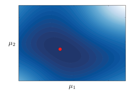
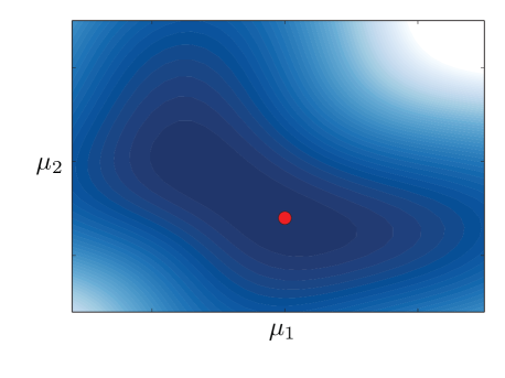
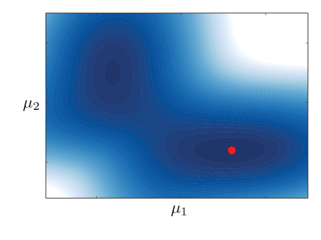
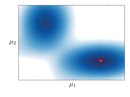
Figure 1: AVI for a mixture model of two Gaussians. We show the variational objective as a function of the two latent Gaussian means $\mu_{0},\mu_{1}$ for temperatures (left to right) $T=20$, $T=13$, $T=8.5$ and $T=1$. The red dot indicates the global optimum.

Interplay of annealing and learning schedules. Our paper treats annealing in a gradient-based setup. Coordinate ascent-based annealing is simpler because there is no learning schedule and therefore the slower we anneal, the better we can track good optima (as can be seen in Fig. 1). In contrast, when following gradients, the temperature schedule and the learning rate schedule become intertwined. When we anneal too slowly, the gradient descent algorithm may approximately converge before the annealed objective has reached its final shape. This leads to suboptimal solutions (e.g., we found in experiments with latent Dirichlet allocation that annealing performs worse than SVI in many cases when temperature is larger than 5). This makes finding good temperature schedules in gradient-based variational annealing hard in practice (finding appropriate learning rates also is hard by itself (Ranganath et al., 2013; Duchi et al., 2011)).

2.3 Variational Tempering (VT)

Since finding an appropriate schedule can be difficult in practice, we focus on adaptive annealing schedules that learn a sequence of temperatures from the data. We build on AVI to develop VT, a method that learns a temperature schedule from the data. VT introduces temperature as an auxiliary variable in the model; it recovers the original model (and thus original posterior) when the temperature is equal to 1.

Random temperatures. As was the case with AVI, VT relies on physical heuristics. It mimics a physical system where several temperatures coexist at the same time, hence where temperature is a random variable that has a joint distribution with the other variables in the system. We consider a finite set of possible temperatures,

$$1\equiv T_{1}<T_{2}<\cdots<T_{M}.$$

A finite, discrete set of temperatures is convenient as it allows us to precompute the tempered partition functions, each temperature leading to a Monte Carlo integral whose dimension does not depend on the data (this is described in Section 3.3).

Multinomial temperature assignments. We introduce a random variable that assigns joint distributions to temperatures. Conditional on the outcome of that random variable, the model is an annealed joint distribution at that temperature. We define a multinomial temperature assignment,

$$y\sim\textrm{Mult}(\pi).$$

We treat $\pi$ as fixed parameters and typically set $\pi_{m}=1/M$.

Tempered joint. The joint distribution factorizes as $p(\mathbf{x},\mathbf{z},\beta,y)=p(\mathbf{x},\mathbf{z},\beta|y)p(y)$. We place a uniform prior over temperature assignments, $p(y)=\prod_{m=1}^{M}\pi_{m}^{y_{m}}$. Conditioned on $y$, we define the tempered joint distribution as

$$p(\mathbf{x},\mathbf{z},\beta|y)=p(\beta)\frac{1}{C(T_{y})}\prod_{i=1}^{N}p(x_{i},z_{i}|\beta)^{1/T_{y}}.$$

This allows us to define the model as

$$p(\mathbf{x},\mathbf{z},\beta,y)=p(\beta)\prod_{m=1}^{M}\left(\frac{\pi_{m}}{C(T_{m})}\prod_{i=1}^{N}p(x_{i},z_{i}|\beta)^{1/T_{m}}\right)^{y_{m}}.$$

The tempered ELBO.

We now define the variational objective for the expanded model. We extend the mean-field family to contain a factor for the temperature,

$$q(\mathbf{z},\beta,y\>|\>\phi,\lambda,r)=q(\mathbf{z}|\phi)q(\beta|\lambda)q(y|r),$$

where we introduced a variational multinomial for the temperature with variational parameter $r$, $q(y|r)=\prod_{m=1}^{M}r_{m}^{y_{m}}$.

Using this family, we augment the annealed ELBO. It now contains terms for the random temperature and explicitly includes $\log C(T)$. The tempered evidence lower bound (T-ELBO) $\mathcal{L}_{T}\equiv\mathcal{L}_{T}(\lambda,\phi,r)$ is

$$\mathcal{L}_{T} = \mathbb{E}_{q}[\log p(\beta)]+\mathbb{E}_{q}[\log p(y)]-{\mathbb{E}}_{q}[\log q(\beta)]$$

$$+\mathbb{E}_{q}[1/T_{y}]{\textstyle\sum_{i}}\mathbb{E}_{q}[\log p(x_{i},z_{i}|\beta)]$$

$$-\mathbb{E}_{q}[\log C(T_{y})]-{\textstyle\sum_{i}}{\mathbb{E}}_{q}[\log q(z_{i})]-\mathbb{E}_{q}[\log q(y)].$$

When comparing the T-ELBO with the annealed ELBO in Eq. 4, we see that expected local inverse temperatures $\mathbb{E}_{q}[1/T_{y}]\equiv{\textstyle\sum_{m}^{M}}\mathbb{E}_{q}[y_{m}/T_{m}]$ in VT play the role of the (global) inverse temperature parameter in AVI. As these expected temperatures typically decrease during learning (as we show), the remaining parts of the tempered ELBO will effectively be annealed over iterations. In VT, we optimize this lower bound to obtain a variational approximation of the posterior.

The tempered partition function. We will now comment on the role of $\log C(T_{y})$ which appears in the T-ELBO (see Eq. 2.3). In contrast to annealing, we cannot omit this term.

Without $C(T_{y})$, the model would place all its probability mass for $m$ around the highest possible temperature $T_{M}$. To see this, note that log likelihoods are generally negative, thus $\mathbb{E}_{q}[\log p(\mathbf{x},\mathbf{z}|\beta)]<0$. If we did not add $-\log C(T_{y})$ to the T-ELBO, maximizing the objective would require us to minimize $\mathbb{E}[1/T_{y}]$.

The log partition function in the T-ELBO prevents temperatures from taking their maximum value. It is usually a monotonically increasing function in $T$. This way $\log C(T_{y})$ penalizes large values of T.

2.4 Local Variational Tempering (LVT)

Instead of working with global temperatures, which are shared across data points, we can define temperatures unique to each data point. This allows us to better fit the data and to learn annealing schedules specific to individual data points. We call this approach local variational tempering (LVT).

In this approach, $T_{i}$ is a per-data point local temperature, and we define the tempered joint as follows:

$$p(\mathbf{x},\mathbf{z},\beta,{\bf T})\propto p(\beta)\prod_{i=1}^{N}\left[p(x_{i},z_{i}|\beta)^{1/T_{i}}p(T_{i})\right].$$ (6)

In the global case, the temperature distribution was limited to discrete support due to normalization. Here we have more flexibility, $p(T_{i})$ can have discrete (multinomial) or continuous support (e.g. $1/T$ could be beta-distributed).

The model can also be formulated as $p(\mathbf{x},\mathbf{z},\beta,{\bf T})=p(\beta)\prod_{i=1}^{N}p(x_{i},z_{i}|\beta/T_{i})p(T_{i}),$ where we see that temperature downweights the global hidden variables and therefore makes the local conditional distributions more entropic. The advantage of this formulation is that we do not have to compute the tempered partition function as the local-tempered likelihood is in the same family as the original one (Section 3). On the downside, the resulting model is non-conjugate.

Local temperature describes the likelihood that a particular data point came from the non-tempered model. Outliers can be better explained in this model by assigning them a high local temperature. $T_{i}$ therefore allows us to more flexibly model the data. It also enables us to learn a different annealing schedule for each data point during inference.

3 Algorithms for Variational Tempering

We now introduce the annealing and variational tempering algorithms for the general class of local and global hidden variables discussed in Section 2.1. Our algorithms are based on stochastic variational inference (Hoffman et al., 2013), a scalable Bayesian inference algorithm that uses stochastic optimization.

3.1 Conditionally Conjugate Exponential Families

As in (Hoffman et al., 2013), we focus on the conditionally conjugate exponential family (CCEF). A model is a CCEF if the prior and local conditional are both in the exponential family and form a conjugate pair,

$$p(\beta|\alpha) = h(\beta)\exp\{\alpha^{\top}t(\beta)-a_{g}(\alpha)\},$$ (7)

$$p(z_{i},x_{i}|\beta) = h(z_{i},x_{i})\exp\{\beta^{\top}t(z_{i},x_{i})-a_{l}(\beta)\}.$$

The functions $t(\beta)=\langle\beta,-a_{l}(\beta)\rangle$ and $t(x_{i},z_{i})$ are the sufficient statistics of the global hidden variables and of the local contexts, respectively. The functions $a_{g}(\cdot)$ and $a_{l}(\cdot)$ are the corresponding log normalizers (Hoffman et al., 2013). Annealed and tempered variational inference apply more generally, but the CCEF allows us to analytically compute certain expectations.

We derive AVI and VT simultaneously. We consider the annealed or tempered ELBO as a function of the global variational parameters,

$${\cal L}(\lambda;T) \triangleq{\cal L}(\lambda,\phi(\lambda;T);T),$$

$$\phi(\lambda;T) \triangleq\rm arg{}\max_{\phi}{\cal L}(\lambda,\phi;T).$$

We have eliminated the dependence on the local variational parameters by implicitly optimizing them in $\phi(\lambda;T)$. This new objective has the same optima for $\lambda$ as the original tempered or tempered ELBO. Following Hoffman et al. (2013), the T-ELBO is

$${\cal L}_{T}(\lambda;T)={\mathbb{E}}_{q}[1/T_{y}]\textstyle{\sum_{i}}({\mathbb{E}}_{q}[t(x_{i},z_{i})]+\alpha)\nabla_{\lambda}a_{g}(\lambda)\\ -\lambda^{\top}\nabla_{\lambda}a_{g}(\lambda)+a_{g}(\lambda)-{\mathbb{E}}_{q}[\log C(T_{y})]-{\mathbb{E}}_{q}[\log q(y)].$$

The annealed ELBO is obtained when replacing $\mathbb{E}_{q(y)}[1/T_{y}]$ by $1/T$ and dropping all other $y-$dependent terms.

Algorithm 1 Annealed or tempered SVI

1:Initialize $\lambda^{(0)}$ randomly. Initialize ${T}>1$.

2:Set the step-size schedule $\rho_{t}$.

3:repeat

4:     Sample a data point $x_{i}$ uniformly. Compute its local variational parameters, $\phi_{t}=\frac{\mathbb{E}_{\lambda_{t}}[\eta_{l}(x_{i}^{(N)},z_{i}^{(N)})]}{{T}}.$

5:     Compute the intermediate global parameters as if $x_{i}$ was replicated $N$ times, $\hat{\lambda}_{t}=\alpha+\frac{1}{{T}}\mathbb{E}_{\phi_{t}}[t(x_{i}^{(N)},z_{i}^{(N)})]$.

6:     Update the current estimate of the global variational parameters, $\lambda_{t+1}=(1-\rho_{t})\lambda_{t}+\rho_{t}\,\hat{\lambda}_{t}.$

7:     Annealing: reduce ${T}$ according to schedule.

8:     Variational Tempering: update ${T}$ with Eq. 9/10.

9:until Forever

3.2 Global and Local Random Variable Updates

To simplify the notation, let $1/T$ either be the deterministic inverse temperature for AVI, or ${\mathbb{E}}[1/T_{y}]$ for VT, or a data point-specific expectation ${\mathbb{E}}[1/T_{i}]$ as for LVT. Following  Hoffman et al. (2013), the natural gradient of the annealed ELBO with respect to the global variational parameters $\lambda$ is

$$\nabla_{\lambda}{\cal L}\;=\;\alpha+\sum_{i=1}^{N}\frac{1}{T}\mathbb{E}_{q}[t(x_{i},z_{i})]-\lambda.$$

The variables $t(x_{i},z_{i})$ are the sufficient statistics from Eq. 7. Setting the gradient to zero gives the corresponding coordinate update for the globals. Because of the structure of the gradient as a sum of many terms, this can be converted into a stochastic gradient by subsampling from the data set, $\hat{\nabla}_{\lambda}{\cal L}=\alpha+\frac{1}{T}\mathbb{E}_{q}[t(x_{i}^{(N)},z_{i}^{(N)})]-\lambda$, where $t(x_{i}^{(N)},z_{i}^{(N)})$ are the sufficient statistics when data point $x_{i}$ is replicated $N$ times. The gradient ascent scheme can also be expressed as the following two-step process,

$$\hat{\lambda}_{t} = \alpha+\frac{1}{{T}}\,\mathbb{E}_{q}[{t(x_{i}^{(N)},z_{i}^{(N)})}],$$

$$\lambda_{t+1} = (1-\rho_{t})\lambda_{t}+\rho_{t}\,\hat{\lambda}_{t}.$$ (8)

We first build an estimate $\hat{\lambda}_{t}$ based on the sampled data point, and then merge this estimate into the previous value $\lambda_{t}$ where $\rho_{t}$ is a decreasing learning rate. In contrast to SVI, we divide the expected sufficient statistics by temperature. This is similar to seeing less data, but also reduces the variance of the stochastic gradient.

After each stochastic gradient step, we optimize the annealed or tempered ELBO over the locals. The updates for the local variational parameters are

$$\phi_{nj}=\frac{1}{{T}}\mathbb{E}_{q}[{\eta_{l}(x_{n},z_{(n,-j)},\beta)}].$$

Above, $\eta_{l}$ is the natural parameter of the original (non-annealed) exponential family distributions of the local variational parameters (Hoffman et al., 2013). As for the globals, the right hand side of the update gets divided by temperature. We found that tempering the local random variable updates is the crucial part in models that involve discrete variables. This initially softens the multinomial assignments and leads to a more uniform and better growth of the global variables.

3.3 Updates of Variational Tempering

We now present the updates specific to VT. In contrast to annealed variational inference, variational tempering optimizes the tempered ELBO, Eq. 2.3. As discussed before, the global and local updates of AVI are obtained from the global and local updates of VT upon substituting $\mathbb{E}_{q(y)}[1/T_{y}]\rightarrow 1/T$. Details on the derivation for these updates are given in the Supplement on the example of LDA.

The temperature update follows from the tempered ELBO. To derive it, consider the log complete conditional for $y$ that is (up to a constant)

$$\log p(y_{m}|\cdot) =y_{m}\left(\frac{1}{T_{m}}\sum_{i}\log p(x_{i},z_{i}|\beta)+\log\frac{\pi_{m}}{C(T_{m})}\right).$$

The variational update for a multinomial variable is

$$r^{*}_{m}\propto\exp\left\{\textstyle\frac{1}{T_{m}}\sum_{i}\mathbb{E}_{q}[\log p(x_{i},z_{i}|\beta)]+\log\frac{\pi_{m}}{C(T_{m})}\right\}.$$ (9)

Let us interpret the resulting variational distribution over temperatures. First, notice that the expected local likelihoods $\mathbb{E}[p(\mathbf{x},\mathbf{z}|\beta)]$ enter the multinomial weights, multiplied with the vector of inverse temperatures. This way, small likelihoods (aka poor fits) favor distributions that place probability mass on large temperatures, i.e. lead to a tempered posterior with large variances. The second term is the log tempered partition function, which is monotonically growing as a function of $T$. As it enters the weights with a negative sign, this term favors low temperatures.

This analysis shows that the distribution over temperatures is essentially controlled by the likelihood: large likelihoods lead to distributions over temperature that place its mass around low temperatures, and vice versa. As likelihoods increase, the temperature distribution shifts its mass to lower values of $T$. This way, the model controls its own annealing schedule. Algorithm 1 summarizes variational tempering.

Estimation of the tempered partition function. Let us sketch how we can approximate the normalization constants $C(T_{m})$ for a discrete set of $T_{m}$. At first sight, this task might seem difficult due to the high dimensionality of the joint. But note that in contrast to the posterior, the joint distribution is highly symmetric, and therefore calculating its normalization is tractable.

In the supplement we prove the following identity for the considered class of CCEF models,

$$C(T_{m})=\int d\beta\,p(\beta)\prod_{i=1}^{N}\left(\int\,dz_{i}\,dx_{i}\,e^{(\beta^{\top}t(x_{i},z_{i})-a_{l}(\beta))/T_{m}}\right)$$

$$\stackrel{{\scriptstyle(A.2)}}{{=}}\int d\beta\,p(\beta)\exp\{-Na_{l}(\beta)/T_{m}+Na_{l}(\beta/T_{m})\}.$$

The dimension of the remaining integral is independent of the size of the data set; it is therefore of much lower dimension than the original integral. We can therefore approximate it by Monte-Carlo integration. We found that $100$ samples are typically enough, each integral typically takes a few seconds in our application. We can alternatively also replace the integral by a MAP approximation (see Supplement A.2). Note that the normalization constants can be precomputed.

3.4 Updates of Local Variational Tempering

For multinomial local temperature variables, the updates are given in analogy to Eq. 9:

$$r^{*}_{m,i}\;\propto\;\exp\left\{\textstyle\frac{1}{T_{m}}\mathbb{E}_{q}[\log p(x_{i},z_{i}|\beta/T_{m})+\log\pi_{m}]\right\}.$$ (10)

Thus, the likelihood’s parameter gets divided by $T$.

In local variational tempering, the global variable is not conjugate due to temperature-specific sufficient statistics. For mean-field variational inference, the variational distribution over the globals would need sufficient statistics of the form $t(\beta)=\left<\beta,-a_{l}(\beta/T_{1}),-a_{l}(\beta/T_{2}),\cdots,-a_{l}(\beta/T_{m})\right>$ which is not conjugate to the model prior, thus we approximate to create a closed-form update.

The first sufficient statistics $\beta$ is shared between our chosen variational approximation and the optimal variational update for the locally tempered model. The second parameter in the variational approximation scales with the number of data points. In the optimal variational update, these data points get split across temperatures. As an approximation, we assign these all to temperature $1$. This results in the following variational update:

$$\hat{\lambda} = \alpha+\mathbb{E}[1/T_{i}]\mathbb{E}[t(x_{i}^{(N)},z_{i}^{(N)})].$$ (11)

This looks the same as the first line in Eq. 3.2 but assigns a different weight to each data point. Thus, in short, we match the first component of the sufficient statistics and pretend it came from a non-tempered model.

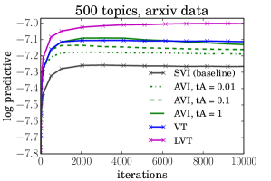
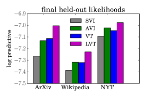
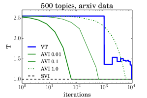
Figure 2: Log predictive likelihoods. We compare SVI (Hoffman et al., 2013), against VT (this paper), LVT (this paper) and AVI (this paper) for different temperature schedules ($tA$ = length of the annealing schedule in effective traversals of the data). Right: temperature schedules for the ArXiv data set.

4 Empirical Evaluation

For the empirical evaluation of our methods, we compare our annealing and variational tempering approaches to standard SVI with latent Dirichlet allocation on three massive text corpora. We also study batch variational inference, AVI, and VT on a factorial mixture model on simulated data and on 2000 images to find latent components. We consider the held-out predictive log likelihood of the approaches (Hoffman et al., 2013). To show that VT and LVT find better local optima in the original variational objective, we predict with the non-tempered model. Deterministic annealing provides a significant improvement over standard SVI. VT performs similarly to the best annealing schedule and further inspection of the automatically learnt temperatures indicate that it approximately recovers the best temperature schedule. LVT (which employs local temperatures) outperforms VT and AVI on all text data sets and was not tested on the factorial model.

Latent Dirichlet allocation. We apply all competing methods to latent Dirichlet allocation (LDA) (Blei et al., 2003). LDA is a model of topic content in documents. It consists of a global set of topics $\beta$, local topic distributions for documents $\theta_{d}$, words $w_{dn}$, and assignments of words to topics $\mathbf{z}$. Integrating out the assignments ${\bf z}$ yields the multinomial formulation of LDA $p(w,\beta,\theta)=\textstyle p(\beta)p(\theta)\prod_{nd}\left(\sum_{k}\theta_{dk}\beta_{kw_{dn}}\right)$. Details on LDA can be found in the Supplement.

Datasets. We studied three datasets: 1.7 million articles collected from the New York Times with a vocabulary of 8,000 words; 640,000 arXiv paper abstracts with a vocabulary of 14,000 words; 3.6 million Wikipedia articles with a vocabulary of 7,702 words. We obtained vocabularies by removing the most and least commonly occurring words.

Hyperparameters and schedules. We used $K=500$ topics and set $\eta$ and $\alpha$ to $1/K$ (we also tested different hyperparameters and found no sensitivity). Larger topic numbers make the optimization problem harder, thus yielding larger improvements of the annealing approaches over SVI. We furthermore set batch size $B=100$ and followed a Robbins-Monro learning rate with $\rho_{t}=(\tau+t)^{-\kappa}$, where $\tau=1024$, $\kappa=0.7$ and $t$ is the current iteration count (these were found to be optimal in (Ranganath et al., 2013)). For SVI we keep temperature at a constant 1. For VT, we distributed $100$ temperatures $1\leq T_{m}\leq 10$ on an exponential scale and initialized $q(y_{n})$ uniformly over the $T_{m}$. We precomputed the tempered partition functions $C(T_{m})$ as discribed in the Supplement. For annealing, we used linear schedules that started in the mean temperature under a uniform distribution over $T_{m}$, and then used a linearly decreasing annealing schedule that ended in $T=1$ after $tA\in\{0.01,0.1,1\}$ effective passes. We updated $T$ every $1000$ iterations. For LVT, we employed $100$ per-document inverse temperatures evenly spaced between $0$ and $1$.

Results We present our results for annealing and variational tempering. We test by comparing the predictive log likelihood of held out test documents. We use half of the words in each document to calculate the approximate posterior distribution over topics then calculate the average predictive probability of the remaining words in the document (following the procedure outlined in (Hoffman et al., 2013)).

Figure 2 shows predictive performance. We see that annealing significantly improves predictive likelihoods with respect to SVI across datasets. In the plot, we index temperature schedules by tA, indicating the number of passes through the dataset. Our results indicate that slow annealing approaches work better (tA=1 is the best performing annealing curve). VT automatically chooses the temperature schedule and is able to recover or improve upon the best annealing curve for arXiv and the New York Times. Variational tempering for Wikipedia is close to that of the best annealing rate, and better than several other manual choices of temperature schedule. In all three cases, LVT gives significantly better likelihoods than AVI and VT.

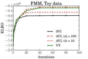
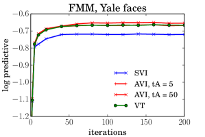
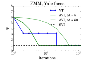
Figure 3: Factorial mixture model (FMM). Left: Evidence lower bound (ELBO) of toy data at $T=1$ for VI (Jordan et al., 1999), annealed VI (AVI, this paper) and variational tempering (VT, this paper). Middle: Log predictive likelihoods on Yale faces. Right: Expected temperatures on Yale faces, as a function of iterations for VI, AVI (linear schedules) and VT.

Factorial mixture model. We also carried out experiments on the Factorial Mixture Model (FMM) (Ghahramani, 1995; Doshi et al., 2009). The model assumes $N$ data points ${\bf X}_{n}\in{\mathbb{R}}^{D}$, $K$ latent components $\mu_{k}\in{\mathbb{R}}^{D}$, and a $K\times N$ binary matrix of latent assignment variables ${\bf Z}_{nk}$. The model has the following generative process (Doshi et al., 2009):

$${\bf X}_{n}\;=\;\sum_{k}{\bf Z}_{nk}{\bf\mu}_{k}+{\bf\epsilon}_{n},\quad{\bf Z}_{nk}\sim{\rm Bern}(\pi_{k}),$$ (12)

$$\mu_{k}\sim{\cal N}(0,\sigma_{\mu}),\quad\epsilon_{n}\sim{\cal N}(0,\sigma_{n}).$$

The variables ${\bf Z}_{nk}$ indicate the activation of factor $\mu_{k}$ in data point $n$. Every ${\bf Z}_{nk}$ is independently $0$ or $1$, which makes the model different from the Gaussian mixture model with categorical cluster assignments. The factorial mixture model is more powerful, but also harder to fit.

We are interested in learning the global variables $\mu_{k}$. We show in the Supplement that the log partition function for the factorial mixture model is

$$\log C(T) = \frac{1}{2}ND\log T+N\sum_{k=1}^{K}\log(\pi_{k}^{1/T}+(1-\pi_{k})^{1/T}).$$

For details on the inference updates, see (Doshi et al., 2009).

Datasets and hyperparameters. We carried out experiments two data sets. The first artificial data set that was generated by first creating $8$ components $\mu_{k}$ by hand. These are $4\times 4$ black and white images, i.e. binary matrices, each of which we weighted with a uniform draw from $[0.5,1]$. (These are shown in Fig. 4.) Given the $\mu_{k}$, we generated 10,000 data points from our model with $\sigma_{n}=0.1$, and $\pi_{k}=0.3$. We set $\sigma_{\mu}=0.35$. Our linear annealing schedule started at $T=10$ and ended in $T=1$ at $10$ and $100$ iterations, respectively. The second data set contained 2000 face images (Yale Face Database B, cropped version) from 28 individuals with $168\times 192$ pixels in different poses and under different light conditions (Lee et al., 2005). We normalized the pixel values by subtracting the mean and dividing by the standard deviation of all pixels. We chose $\sigma_{n}=\sigma_{\mu}=0.5$ which we found to perform best. Our annealing curves start at $T=6$ and end in $T=1$ after $5$ and $50$ iterations, respectively. Since both datasets were comparatively small, we used batch updates.

Results. Fig. 4 shows the results when comparing variational inference, annealed VI, and VT on the artificial data. The left plot shows the ELBO at $T=1$. As becomes apparent, AVI and VT converge to better local optima of the original non-tempered objective. The plots on the right are the latent features $\mu_{k}$ that are found by the algorithm. Variational tempering finds much cleaner features that agree better with the ground truth than VI, which gets stuck in a poor local optimum. Fig. 3 shows held-out likelihoods for the Yale faces dataset. Among the 2000 images, 500 were held out for testing. VT automatically finds an annealing schedule that comes close to the best linear schedule that we found. The plot on the right shows the different temperature schedules.

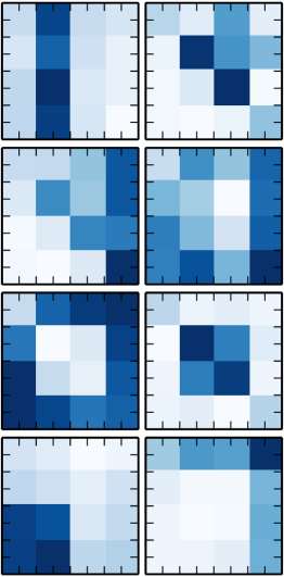
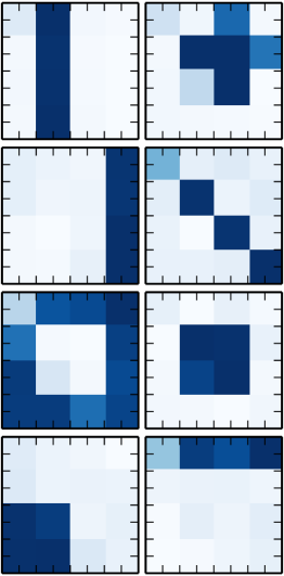
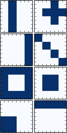
(a)       (b)       (c)

Figure 4: FMM on toy data. The shapes on the bottom show the latent global variables as found by (a) variational inference (Jordan et al., 1999) and (b) variational tempering (this paper). Figure (c) shows the ground truth that was used to generate the data.

5 Conclusions

We presented three temperature based algorithms for variational inference: annealed variational inference and global variational tempering, and local variational tempering. All three algorithms scale to large data, result in higher predictive likelihoods, and can be generalized to a broader class of models using black box variational methods. VT requires model-specific precomputations but results in near-optimal global temperature schedules. As such, AVI and LVT may be easier to use. An open problem is to characterize and avoid new local optima that may be created when treating temperature as a latent variable in variational inference.

Acknowledgements.

This work is supported by NSF IIS-0745520, IIS-1247664, IIS-1009542, ONR N00014-11-1-0651, DARPA FA8750-14-2-0009, N66001-15-C-4032, Facebook, Adobe, Amazon, NVIDIA, and the Seibel and John Templeton Foundations.

Supplementary Material

Appendix A Tempered Partition Functions

Variational Tempering requires that we precompute the tempered partition functions for a finite set of pre-specified temperatures:

$$C(T) = \int d\beta p(\beta)\prod_{i=1}^{N}\left(\int dx_{i}dz_{i}p(x_{i},z_{i}|\beta)^{1/T}\right).$$ (13)

We first show how to reduce this to an integral only over the globals. Because the size of the remaining integration is independent of $N$, it is tractable by Monte-Carlo integration with a few hundred to thousand samples.

A.1 Generic model.

Here we consider a generic latent variable model of the SVI class, i.e. containing local and global hidden variables. The following calculation reduces the original integral over global and local variables to an integral over the global variables alone:

$$C(T) = \int d\mathbf{x}\,d\mathbf{z}\,d\beta\,p(\beta)p(\mathbf{z},\mathbf{x}|\beta)^{1/T}$$

$$= \int d\beta\,p(\beta)\prod_{i=1}^{N}\left(\int dx_{i}\,dz_{i}\,p(x_{i},z_{i}|\beta)^{1/T}\right)$$

$$= \int d\beta\,p(\beta)\prod_{i=1}^{N}\left(\int\,dz_{i}\,dx_{i}\,\right.$$

$$\left.\quad\quad\quad\times\exp\{T^{-1}\beta t(x_{i},z_{i})-T^{-1}a_{l}(\beta)\}\right).$$

We now use the following identity:

$$\int\,dz_{i}\,dx_{i}\,\exp\{T^{-1}\beta t(x_{i},z_{i})-T^{-1}a_{l}(\beta)\}$$

$$= \int\,dz_{i}\,dx_{i}\,e^{\;T^{-1}\beta t(x_{i},z_{i})-T^{-1}a_{l}(\beta)+a_{l}(T^{-1}\beta)-a_{l}(T^{-1}\beta)}$$

$$= e^{-T^{-1}a_{l}(\beta)+a_{l}(T^{-1}\beta)}\underbrace{\int\,dz_{i}\,dx_{i}\,e^{\;T^{-1}\beta t(x_{i},z_{i})-a_{l}(T^{-1}\beta)}}_{=1}$$

$$= \exp\{-T^{-1}a_{l}(\beta)+a_{l}(T^{-1}\beta)\}.$$

Note that the integral is independent of $i$, as all data points contribute the same amount to the tempered partition function. Combining the last 2 equations yields

$$C(T) = \int d\beta\,p(\beta)\exp\{-NT^{-1}a_{l}(\beta)+Na_{l}(T^{-1}\beta)\}.$$

The complexity of computing the remaining integral does not depend on the number of data points, and therefore it is tractable with simple Monte-Carlo integration. We approximate the integral as is

$$\log C(T)\approx\log\frac{1}{N_{s}}\sum_{\beta\sim p(\beta)}\exp\left\{-NT^{-1}a_{l}(\beta)+Na_{l}(T^{-1}\beta)\right\}.$$

For the models under consideration, we found that typically less than 100 samples suffice. In more complicated setups, more advances methods to estimate the Monte Carlo integral can be used, such as annealed importance sampling. While we typically precompute the tempered partition function for about 100 values of T, the corresponding computation could easily be incorporated into the variational tempering algorithm.

Analytic approximation.

Instead of precomputing the log partition function, one could also use an analytic approximation for sparse priors with a low variance (this approximation was not used in the paper). In this case, we can MAP-approximate the $\beta-$integral, which results in

$$\log C(T) \approx N\left(T^{-1}a_{l}(\beta^{*})-a_{l}(T^{-1}\beta^{*})\right).$$ (15)

For large data, this approximation gets better and yields an analytic result.

Appendix B Latent Dirichlet Allocation

B.1 Tempered partition function

We now demonstrate the calculation of the tempered partition function on the example of Latent Dirichlet Allocation (FFM). We use the multinomial representation of LDA where the topic assignments are integrated out,

$$p(w,\beta,\theta)=p(\beta)p(\theta)\prod_{nd}\left(\sum_{k}\theta_{dk}\beta_{kw_{dn}}\right).$$ (16)

The probability that word $w_{dn}$ is the multinomial parameter $\sum_{k}\theta_{dk}\beta_{kw_{dn}}$. In this formulation, LDA relates to probabilistic matrix factorization models.

LDA uses Dirichlet priors $p(\theta)=\prod_{d}\text{Dir}(\theta_{d}|\alpha)$ and $p(\beta)=\prod_{k}\text{Dir}(\beta_{k}|\eta)$ for the global variational parameters $\beta$ and the per-document topic proportions $\theta$.

The inner ”integral” over $w_{dn}$ is just the sum over the multinomial mean parameters,

$$\int d{w_{dn}}\;p(w_{dn}|\theta_{d},\beta)^{1/T} = \sum_{v=1}^{V}\left(\sum_{k}\theta_{dk}\beta_{kv}\right)^{1/T}.$$ (17)

The tempered partition function for LDA is therefore

$$C(T) =\int d\beta p(\beta)\prod_{d=1}^{D}\int d\theta_{d}p(\theta_{d})\left(\sum_{v}\left(\sum_{k}\theta_{dk}\beta_{kv}\right)^{1/T}\right)^{N_{d}}$$

$$\approx\int d\beta p(\beta)\left(\int d\theta\,p(\theta)\left(\sum_{v}\left(\sum_{k}\theta_{k}\beta_{kv}\right)^{1/T}\right)^{N}\right)^{D},$$

where as usual $N=W/D$ is the approximate number of words per document. The corresponding Monte-Carlo approximation for the log partition function is

$$\log C(T) \approx \log\frac{1}{N_{\beta}}\sum_{\beta\sim p(\beta)}\exp\{D\log\frac{1}{N_{\theta}}$$

$$\times\sum_{\theta\sim p(\theta)}\exp(N\log\sum_{v}(\sum_{k}\theta_{k}\beta_{kv})^{1/T}))\}.$$

$N_{\theta}$ and $N_{\beta}$ are the number of samples from $p(\theta)$ and $p(\beta)$, respectively. To bound the log partition function we can now apply Jensen’s inequality twice: Once for the concave logarithm, and once in the other direction for the convex functions $x\rightarrow x^{D}$ and $x\rightarrow x^{N}$:

$$\log C(T)\geq N\cdot D\int d\beta p(\beta)\int d\theta p(\theta)\log\sum_{v}\left(\sum_{k}\theta_{k}\beta_{kv}\right)^{1/T},$$

$$\log C(T)\leq N\cdot D\log\int d\beta p(\beta)\int d\theta p(\theta)\sum_{v}\left(\sum_{k}\theta_{k}\beta_{kv}\right)^{1/T}.$$

We see that the log partition function scales with the total number of observed words $N\times D$, This is conceptually important because otherwise $\log C(T)$ would have no effect on the updates in the limit of large data sets.

B.2 Variational updates

In its formulation with the local assignment variables $z_{n}$, the LDA model is

$$p(w,z,\beta,\theta)=p(\beta)p(\theta)\prod_{n,d,k}\exp\{z_{dnk}(\log\theta_{dk}+\log\beta_{kw_{dn}})\}.$$

Let $N_{tot}$ be overall the number of words in the corpus, $N_{d}$ the number of words in document $d$, $D$ the number of documents, and $K$ the number of topics. We have that $\sum_{d=1}^{D}N_{d}=N_{tot}$. The tempered model becomes

$$p(w,z,\beta,\theta,y)=p(\beta)p(\theta)\prod_{m}\times\\ \exp\{y_{m}\left[\sum_{n,d,k}z_{dnk}\frac{\log\theta_{dk}+\log\beta_{kw_{dn}}}{T_{m}}-\log C(T_{m})\right]\}.$$

where $m$ indexes temperatures.

Variational updates.

We obtain the following optimal variational distributions from the complete conditionals (all up to constants). We replaced sums over word indices $n$ by sums over the vocabulary indices $v$, weighted with word counts $n_{dv}$:

$$\log q^{*}(z_{dvk}) =z_{dvk}n_{dv}{\mathbb{E}}[1/T_{y}]({\mathbb{E}}[\log\theta_{dk}]+{\mathbb{E}}[\log\beta_{kv}]),$$ (19)

$$\log q^{*}(y_{m}) =y_{m}\left[\frac{1}{T_{m}}\sum_{vk}n_{dv}\,{\mathbb{E}}[z_{dvk}]({\mathbb{E}}[\log\theta_{dk}]\right.$$

$$+\left.{\mathbb{E}}[\log\beta_{kv}])-{\mathbb{E}}[\log C(T_{y})]\right],$$

$$\log q^{*}(\theta_{dk}) =\log\theta_{dk}\left(\sum_{v}n_{dv}\,{\mathbb{E}}[1/T_{y}]{\mathbb{E}}[z_{dvk}]+\alpha\right),$$

$$\log q^{*}(\beta_{kv}) =\log\beta_{kv}\left(\sum_{d}n_{dv}\,{\mathbb{E}}[1/T_{y}]{\mathbb{E}}[z_{dvk}]+\eta\right).$$

Appendix C Tempered Partition function for the Factorial Mixture Model

We apply variational tempering to the factorial mixture model (FMM) as described in the main paper,

$$p({\bf X},{\bf Z},\mu,\pi|\alpha,\mu_{0}) = p({\bf X}|{\bf Z},\mu,\sigma_{n})p({\bf Z}|\pi)p(\mu|\sigma_{\mu}).$$

For convenience, we define the assigned cluster means for each data point:

$$\mu_{n}({\bf Z}) = \sum_{k}{\bf Z}_{nk}\mu_{k}.$$ (20)

The data generating distribution for the FMM is now a product over $D-$dimensional Gaussians:

$$p({\bf X}|{\bf Z},\mu,\sigma_{n}) = \prod_{n}{\cal N}({\bf X}_{n};\mu_{n}({\bf Z}),\sigma_{n}{\bf I}_{D})$$ (21)

The local conditional distribution also involves the prior $\prod_{n}p({\bf Z}_{n}|\pi)$ of hidden assignments,

$$p({\bf X},{\bf Z}|\mu,\sigma_{n}) = \prod_{n}{\cal N}({\bf X}_{n};\mu_{n}({\bf Z}),\sigma_{n}{\bf I}_{D})p({\bf Z}_{n}|\pi).$$

Here is the tempered local conditional:

$$p({\bf X},{\bf Z}|\mu,\pi)^{1/T}=\prod_{n}\frac{1}{\sqrt{(2\pi\sigma_{n})^{D}}}\\ \times\exp\left\{-\frac{1}{2\sigma_{n}T}\sum_{n}({\bf X}_{n}-\mu_{n})^{\top}({\bf X}_{n}-\mu_{n})+\frac{1}{T}\log p({\bf Z}_{n}|\pi)\right\}.$$

When computing the tempered partition function, we need to integrate out all variables, starting with the locals. We can easily integrate out ${\bf X}$; this removes the dependence on $\mu$ which only determines the means of the Gaussians:

$$C(T,{\bf Z},\pi) = \int d^{D}{\bf X}\;p({\bf X},{\bf Z}|\mu,\pi)^{1/T}$$

$$= \left(\prod_{n=1}^{N}\frac{\sqrt{(2\pi\sigma_{n}T)^{D}}}{\sqrt{(2\pi\sigma_{n})^{D}}}\right)\prod_{n}p({\bf Z}_{n}|\pi)^{1/T}$$

$$= \sqrt{T}^{ND}\prod_{n}p({\bf Z}_{n}|\pi)^{1/T}.$$

Hence, integrating the tempered Gaussians removes the $\mu-$dependence and gives an analytic contribution $\sqrt{T}^{ND}$ to the tempered partition function. It remains to compute

$$C(T) = \sqrt{T}^{ND}\int d{\bf Z}\prod_{n}p({\bf Z}_{n}|\pi)^{1/T}.$$ (23)

Since the Bernoulli variables are discrete, the last marginalization yields

$$\sum_{\{{\bf Z}_{nk}\}}\prod_{nk}\pi_{k}^{{\bf Z}_{nk}/T}(1-\pi_{k})^{(1-{\bf Z}_{nk})/T}$$ (24)

$$= \prod_{nk}\sum_{\{{\bf Z}_{nk}=\pm 1\}}\pi_{k}^{{\bf Z}_{nk}/T}(1-\pi_{k})^{(1-{\bf Z}_{nk})/T}$$

$$= \prod_{k}\left(\pi_{k}^{1/T}+(1-\pi_{k})^{1/T}\right)^{N}.$$

Finally, the log tempered partition function is

$$\log C(T) = \frac{1}{2}ND\log(T)+N\sum_{k}\log\left(\pi_{k}^{1/T}+(1-\pi_{k})^{1/T}\right)$$

$$= \frac{1}{2}ND\log(T)+NK\log\left(\pi^{1/T}+(1-\pi)^{1/T}\right).$$

In the last line we used that the hyperparameters $\pi_{k}\equiv\pi$ are isotropic in $K-$space.

References

- Berg and Neuhaus (1992) Berg, B. A. and Neuhaus, T. (1992). Multicanonical ensemble: A new approach to simulate first-order phase transitions. Physical Review Letters, 68(1):9.
- Blei et al. (2003) Blei, D. M., Ng, A., and Jordan, M. I. (2003). Latent Dirichlet allocation. Journal of Machine Learning Research, 3:993-1022.
- Doshi et al. (2009) Doshi, F., Miller, K., Gael, J. V., and Teh, Y. W. (2009). Variational inference for the Indian buffet process. In International Conference on Artificial Intelligence and Statistics, pages 137–144.
- Duchi et al. (2011) Duchi, J., Hazan, E., and Singer, Y. (2011). Adaptive subgradient methods for online learning and stochastic optimization. Journal of Machine Learning Research, 12:2121–2159.
- Geyer (1991) Geyer, C. J. (1991). Markov chain Monte Carlo maximum likelihood. In Interface Proceedings.
- Ghahramani (1995) Ghahramani, Z. (1995). Factorial learning and the EM algorithm. In Advances in Neural Information Processing Systems, pages 617–624.
- Ghahramani and Hinton (2000) Ghahramani, Z. and Hinton, G. E. (2000). Variational learning for switching state-space models. Neural computation, 12(4):831–864.
- Hoffman et al. (2013) Hoffman, M. D., Blei, D. M., Wang, C., and Paisley, J. (2013). Stochastic variational inference. Journal of Machine Learning Research, 14(1):1303–1347.
- Jordan et al. (1999) Jordan, M. I., Ghahramani, Z., Jaakkola, T. S., and Saul, L. K. (1999). An introduction to variational methods for graphical models. Machine Learning, 37(2):183–233.
- Katahira et al. (2008) Katahira, K., Watanabe, K., and Okada, M. (2008). Deterministic annealing variant of variational bayes method. Journal of Physics: Conference Series, 95(1):012015.
- Kirkpatrick et al. (1983) Kirkpatrick, S., Gelatt, C. D., Vecchi, M. P., et al. (1983). Optimization by simmulated annealing. Science, 220(4598):671–680.
- Lee et al. (2005) Lee, K.-C., Ho, J., and Kriegman, D. J. (2005). Acquiring linear subspaces for face recognition under variable lighting. Pattern Analysis and Machine Intelligence, IEEE Transactions on, 27(5):684–698.
- Marinari and Parisi (1992) Marinari, E. and Parisi, G. (1992). Simulated tempering: a new Monte Carlo scheme. EPL (Europhysics Letters), 19(6):451.
- McInerney et al. (2015) McInerney, J., Ranganath, R., and Blei, D. (2015). The population posterior and Bayesian modeling on streams. In Advances in Neural Information Processing Systems, pages 1153–1161.
- Metropolis et al. (1953) Metropolis, N., Rosenbluth, A. W., Rosenbluth, M. N., Teller, A. H., and Teller, E. (1953). Equation of state calculations by fast computing machines. The Journal of Chemical Physics, 21(6):1087–1092.
- Neal (1993) Neal, R. M. (1993). Probabilistic inference using Markov chain Monte Carlo methods. Department of Computer Science, University of Toronto Toronto, Ontario, Canada.
- Ranganath et al. (2013) Ranganath, R., Wang, C., Blei, D. M., and Xing, E. P. (2013). An adaptive learning rate for stochastic variational inference. In In International Conference on Machine Learning.
- Rose et al. (1990) Rose, K., Gurewitz, E., and Fox, G. (1990). A deterministic annealing approach to clustering. Pattern Recognition Letters, 11(9):589–594.
- Swendsen and Wang (1986) Swendsen, R. H. and Wang, J.-S. (1986). Replica Monte Carlo simulation of spin-glasses. Physical Review Letters, 57(21):2607.
- Ueda and Nakano (1998) Ueda, N. and Nakano, R. (1998). Deterministic annealing em algorithm. Neural Networks, 11(2):271–282.
- Wainwright and Jordan (2005) Wainwright, M. J. and Jordan, M. I. (2005). A variational principle for graphical models. In New Directions in Statistical Signal Processing: From Systems to Brain. MIT Press.
- Yoshida and West (2010) Yoshida, R. and West, M. (2010). Bayesian learning in sparse graphical factor models via variational mean-field annealing. Journal of Machine Learning Research, 11:1771–1798.