Noncommutative minisuperspace, gravity-driven acceleration and kinetic inflation

Abstract

In this paper, we introduce a noncommutative version of the Brans-Dicke (BD) theory and obtain the Hamiltonian equations of motion for a spatially flat Friedmann–Lemaître–Robertson–Walker universe filled with a perfect fluid. We focus on the case where the scalar potential as well as the ordinary matter sector are absent. Then, we investigate gravity-driven acceleration and kinetic inflation in this noncommutative BD cosmology. In contrast to the commutative case, in which the scale factor and BD scalar field are in a power-law form, in the noncommutative case the power-law scalar factor is multiplied by a dynamical exponential warp factor. This warp factor depends on the noncommutative parameter as well as the momentum conjugate associated to the BD scalar field. We show that the BD scalar field and the scale factor effectively depend on the noncommutative parameter. For very small values of this parameter, we obtain an appropriate inflationary solution, which can overcome problems within BD standard cosmology in a more efficient manner. Furthermore, a graceful exit from an early acceleration epoch towards a decelerating radiation epoch is provided. For late times, due to the presence of the noncommutative parameter, we obtain a zero acceleration epoch, which can be interpreted as the coarse-grained explanation.

I Introduction

Among the theories alternative to Einstein’s general relativity, the Brans-Dicke (BD) theory BD61 is the simplest and the best known. In the BD theory, the gravitational constant has been assumed to be a dynamical variable, which is proportional to the inverse of a dynamical scalar field, namely, the BD scalar field, $\phi$.

In the Jordan frame of the BD theory, the scalar field couples nonminimally only with the geometry and does not couple directly with the matter. Hence, the energy-momentum tensor of the ordinary matter (all types of matter except the BD scalar field) obeys the usual conservation law. Moreover, there is a free dimensionless adjustable parameter, which is called the BD coupling parameter and denoted by $\omega$. In spite of the theoretical proposals in which it has been anticipated that the values of the BD parameter should be of order unity, observational measurements have indicated that the lower bound on $\mid\omega\mid$ is large Faraoni.book .

At a classical level, to obtain results in agreement with observational data, for an early as well as a late time universe, other extended versions of the BD theory (scalar-tensor theories) have been applied. In these theories, in contrary to the standard version of the BD theory, it has been assumed that either the BD coupling parameter should be a general function of the BD scalar field BP01 , and/or a scalar potential MC07 (which is also a function of $\phi$) must be added by hand. It is also established that the BD theory not only can provide observational consequences to convince the original aims of the theory, but also it is possible to construct interesting quantum cosmological models, which may present appropriate scenarios to study the inflationary universe LS89-SA90-S98-CL11-CFPS12 ; BM90 .

In the BD setting of Lev95 ; Lev95-2 , which is of interest in this study, an accelerated expanding universe was not obtained by adding a scalar potential or a cosmological constant. However, contrary to the standard BD theory, a variable BD coupling parameter rather than a constant one has been assumed. Being more concrete, an accelerated expanding universe emerges from the kinetic energy density of a dynamical Planck mass without introducing any scalar potential or cosmological constant. More precisely, in this formalism, the pressure associated to the kinetic energy density is negative.

Although having an accelerating scale factor is required to explain the early as well as late time phases of the Universe, additional features need to be satisfied. In fact, the early Universe must inflate such that it can overcome the problems with the standard cosmology. Moreover, a successful inflationary model must exit from an accelerating phase and proceed to a decelerated expansion.

In Ref. Lev95-2 , it has been shown that, to meet sufficient inflation, it is required to have an accelerating scale factor in the Einstein frame. However, there is no source to get an accelerating scale factor in that frame in the model investigated in Lev95-2 . Thus, kinetic inflation, even by assuming a variable BD coupling parameter, cannot lead to today’s Universe. Namely, in the commutative case of the BD theory (in the Jordan frame), there is an important problem with kinetic inflation, even with a variable $\omega$: regardless of the form of $\omega(\phi)$, all the D branch solutions are encountered with the graceful exit problem Lev95-2 . The graceful exit problem is also an obstacle in (accelerated) inflation within more general solutions in the context of string theory BV94 .

In this work, we will present a model which can give an accelerating scale factor for the early Universe, without encountering the above-mentioned problems. Moreover, we will show that the nominal as well as sufficient conditions, which are required for an inflationary epoch, are satisfied in a more convenient manner when the noncommutativity parameter is present. Our model will not be constructed by adding a scalar potential or by taking a variable BD coupling parameter. Instead, we will study the effects of a noncommutativity in a cosmology constructed with a flat Friedmann–Lemaître–Robertson–Walker (FLRW) model in the context of the BD theory, in the absence of the ordinary matter.

Noncommutative field theory CDS98-SW99-DN01 has been applied to gravitational models which led to present a few noncommutative proposals for gravity GORS03-GORS03-2-ADMW06-EGOR08 . Such approaches have indicated that their corresponding noncommutative field equations are very complicated to solve. However, by applying some arguments, gravitational models based on noncommutativity with simplified field equations involving noncommutative effects have been obtained. Basically, by means of applying an effective noncommutativity on a minisuperspace, the noncommutative deformations of the minisuperspace can be investigated at the quantum level. At the classical level, noncommutative deformations have also been studied; see, e.g. BP04-PM05-AAOSS07-GSS07 ; GSS11 ; RFK11 ; RZMM14 .

The major objective of this paper will be to construct the spatially flat FLRW field equations for a generalized BD theory by means of the Hamiltonian formalism in a noncommutativite minisuperspace. Then, we proceed to obtain the solutions for very special cases and investigate the effects of noncommutativity. By introducing a noncommutative Poisson bracket between the BD scalar field and the logarithm of scale factor, we will construct a noncommutative BD cosmology. The effects of such a noncommutativity on the BD vacuum solutions are discussed.

Our paper is, therefore, organized as follows. In Sec. II, the general Hamiltonian equations of motion for an extended version of a BD theory (in Jordan frame) in the presence of a special kind of a noncommutativity for a spatially flat FLRW universe are derived. In Sec. III, we restrict ourselves to solve the field equations for a case in which there is not a scalar potential or an ordinary matter. In Sec. IV, we will argue that the obtained solutions in section III can be a successful alternative for a kinetic inflationary model. In Sec. V, we will summarize and analyze the results of the paper.

II Noncommutative Cosmological equations in Brans-Dicke Theory

Let us start with the spatially flat FLRW metric as the background geometry, namely

$$ds^{2}=-N^{2}(t)dt^{2}+e^{2\alpha(t)}\left(dx^{2}+dy^{2}+dz^{2}\right),$$ (1)

where $N(t)$ is a lapse function and $a(t)=e^{\alpha(t)}$ is the scale factor. We will work with a Lagrangian density of the BD theory in the Jordan frame BD61 ; Jordan55-FGN99 as

$${\cal L}[\gamma,\phi] = \sqrt{-\gamma}\left[\phi R-\frac{\omega}{\phi}\gamma^{\mu\nu}\nabla_{\mu}\phi\nabla_{\nu}\phi-V(\phi)\right]$$

$$+ \sqrt{-\gamma}{\cal L_{\rm matt}},$$

where the greek indices run from zero to $3$, and ${\cal L_{\rm matt}}=16\pi\rho(\alpha)$ (where $\rho$ is the energy density) is the Lagrangian density associated to the ordinary matter. In order to have an attractive gravity, we should notice that the BD scalar field $\phi$ must take positive values. $V(\phi)$ is the scalar potential, and $R$ is the Ricci scalar associated to the metric $\gamma_{\mu\nu}$, whose determinant was denoted by $\gamma$. In this work, we will assume the BD coupling parameter $\omega$ to be a constant and, in vacuum, requiring stability in Lorentzian space, it must be restricted as $\omega>-3/2$ C98 ; BKM04-DDB07-BS07-B09 . It is straightforward to show that the Hamiltonian of the model is given by

$${\cal H}\!\!\! = \!\!\!-\frac{Ne^{-3\alpha}}{2(2\omega+3)\phi}\left(\frac{\omega}{6}P_{\alpha}^{2}-\phi^{2}P_{\phi}^{2}+\phi P_{\alpha}P_{\phi}\right)$$

$$+ \!\!\!Ne^{3\alpha}\left(V-16\pi\rho\right),$$

where $P_{\alpha}$ and $P_{\phi}$ are the conjugate momenta associated to the $\alpha$ and $\phi$, respectively. We will be working with the comoving gauge; namely, we have set $N(t)=1$. Thus, by applying the above Hamiltonian, the equations of motion corresponding to the phase space coordinates $\{\alpha,\phi;P_{\alpha},P_{\phi}\}$, in which the Poisson algebra is $\{\alpha,\phi\}=0$, $\{P_{\alpha},P_{\phi}\}=0$, $\{\alpha,P_{\alpha}\}=1$ and $\{\phi,P_{\phi}\}=1$, are given by

$$\dot{\alpha}\!\! = \!\!-\frac{e^{-3\alpha}}{2(2\omega+3)\phi}\left(\frac{\omega}{3}P_{\alpha}+\phi P_{\phi}\right),$$ (4)

$$\dot{P_{\alpha}}\!\! = \!\!e^{3\alpha}\left[-6V+16\pi\left(6\rho+\frac{d\rho}{d\alpha}\right)\right],$$ (5)

$$\dot{\phi}\!\! = \!\!-\frac{e^{-3\alpha}}{2(2\omega+3)}\left(P_{\alpha}-2\phi P_{\phi}\right),$$ (6)

$$\dot{P_{\phi}}\!\! = \!\!\frac{e^{-3\alpha}}{2(2\omega+3)\phi}\left(P_{\alpha}-2\phi P_{\phi}\right)P_{\phi}$$

$$- \!\!\!\frac{e^{3\alpha}}{\phi}\left(V+\phi\frac{dV}{d\phi}-16\pi\rho\right),$$

where a dot denotes the differentiation with respect to the cosmic time. Because of the homogeneous and isotropic FLRW universe choice, we have assumed that the spatial gradients in the BD scalar field are negligible, namely, $\phi=\phi(t)$. By using the equation of state associated to a perfect fluid and the Hamiltonian constraint, it is straightforward to derive the usual FLRW field equations in the context of the BD cosmology. However, in this paper, we prefer to work with the first order Hamiltonian differential equations.

We will investigate the effects of noncommutativity in this cosmological model. In fact, in order to achieve the corresponding FLRW equations for a noncommutative setting, we should begin from a noncommutative theory of gravity. However, as performing such a procedure is a complicated process, it is usually replaced by an effective noncommutativity in the minisuperspace COR02 ; BP04-PM05-AAOSS07-GSS07 . By modifying the Poisson algebra, some particular noncommutative frameworks have been applied to a minimally coupled scalar field cosmology GSS11 , namely, in quantum cosmology. In particular, a dynamical deformation between the momenta associated to the scale factor and scalar field has been used in both of nonminimally and minimally coupled scalar field cosmology to discuss the corresponding effects in the evolution of the Universe and singularity formation RFK11 ; RZMM14 .

In order to investigate the effects of a classical evolution of the noncommutativity on the cosmological equations of motion in the BD theory, we propose the following Poisson commutation relations between the variables:

$$\{\alpha,\phi\}=\theta,\hskip 28.45274pt\{P_{\alpha},P_{\phi}\}=0,$$ (8)

$$\{\alpha,P_{\alpha}\}=1,\hskip 28.45274pt\{\phi,P_{\phi}\}=1,$$

where the noncommutative parameter $\theta$ is a constant. Applying the commutation relations (8) leads us to the following deformed equations of motion

$$\dot{\alpha}\!\!\! = \!\!\!-\frac{e^{-3\alpha}}{2(2\omega+3)\phi}\left[\frac{\omega}{3}P_{\alpha}+\phi P_{\phi}\!+\!\theta(P_{\alpha}-2\phi P_{\phi})P_{\phi}\right]$$ (9)

$$+ \theta\left(\frac{e^{3\alpha}}{\phi}\right)\left[V(\phi)+\phi\frac{dV(\phi)}{d\phi}-16\pi\rho\right],$$

$$\dot{\phi}\!\! = \!\!-\frac{e^{-3\alpha}}{2(2\omega+3)}\left(P_{\alpha}-2\phi P_{\phi}\right)$$ (10)

$$- 6\theta e^{3\alpha}\left[V(\phi)-16\pi\left(\rho+\frac{1}{6}\frac{d\rho}{d\alpha}\right)\right],$$

where, as the equations of motion associated to the momenta $P_{\rm a}$ and $P_{\rm\phi}$ under the proposed noncommutative deformation do not change, we have abstained from rewriting them. Equations (9) and (10) together with those for the momenta, namely, Eqs. (5) and (II), are the Hamiltonian equations for the noncommutative BD setting, and obviously, the standard commutative equations are recovered in the limit $\theta\rightarrow 0$.

In the next sections, we investigate the cosmological implications of this model for a very simple case in which the scalar potential and the ordinary matter are absent.

III Gravity-Driven acceleration for cosmological models in the commutative and noncommutative BD theory

Let us assume a very simple case in which we set $\rho=0$ and $V(\phi)=0$. In the commutative setting of BD theory, such a model has been considered as an appropriate approach in which the key ideas of the duality and branch changing have been studied L97 . In addition, as mentioned, a gravity-driven acceleration epoch is obtained without introducing any scalar potential, cosmological constant, and/or ordinary matter. In the commutative case, such solutions, by assuming a variable BD coupling parameter, have been investigated in detail in Refs. Lev95 ; Lev95-2 . In what follows, we will study the effects of a constant noncommutative parameter introduced by relation (8) on the behavior of the cosmological quantities. We should remind that, in contrast to the approaches of Lev95 ; Lev95-2 , we have assumed the original BD theory in which $\omega$ should be a constant. As we will see, the presence of the noncommutative parameter leads us to some interesting consequences.

In the absence of the scalar potential and ordinary matter, from (5) we get $\dot{P_{\alpha}}=0$, which gives a constant of motion and may assist us to solve the rest of the equations of motion. Thus, we get $P_{\alpha}=c_{1}$; also, Eqs. (II) and (9) give $P_{\phi}=c_{2}^{\pm}\phi^{-1}$ where $c_{1}$ and $c_{2}^{\pm}\neq 0$ are the integration constants. These constants are not independent; by substituting them into the Hamiltonian constraint, we get the following relation between them:

$$c^{\pm}_{1}=\frac{3|c_{2}|}{\omega}\left[-{\rm sgn}(c_{2})\pm\xi\right],$$ (11)

where $\omega\neq 0$, $\xi\equiv\sqrt{1+2\omega/3}$, and ${\rm sgn}(x)=x/|x|$ is the signum function. Thus, from (10), $\dot{\phi}$ is written as

$$\dot{\phi}=-\frac{f^{\pm}}{\xi a^{3}}\hskip 14.22636pt{\rm where}\hskip 14.22636ptf^{\pm}\equiv\frac{|c_{2}|}{2\omega}\left[-{\rm sgn}(c_{2})\xi\pm 1\right].$$ (12)

By employing the obtained expressions associated to the momenta and the integration constants, Eqs. (9) and (10) lead us to

$$H=h^{\pm}\left(\frac{\dot{\phi}}{\phi}\right)\hskip 14.22636pt{\rm where}\hskip 14.22636pth^{\pm}\equiv g^{\pm}+\frac{c_{2}\theta}{\phi},$$ (13)

$H=\dot{a}/a$ is the Hubble constant and $g^{\pm}$ is given by

$$g^{\pm}\equiv-\frac{1}{2}\left[1\pm{\rm sgn}(c_{2})\xi\right].$$ (14)

Notice that the above equations corresponding with each sign of $c_{2}$ give two branches for the Hubble parameter. As we have assumed $\phi>0$, i.e., an attractive gravity Faraoni.book , in order to discuss an expansion or contraction, the values of $\dot{\phi}$ as well as $h$ corresponding to each branch must be considered. For instance, by considering a special case by supposing $c_{2}>0$ and $\theta=0$, we get $H=-1/2\left(\dot{\phi}/\phi\right)(1\pm\xi)$. In this case, for $\xi<1$, $H>0$ only when $\dot{\phi}<0$, and $H<0$ only when $\dot{\phi}>0$ (for both of the branches). While, for $\xi>1$, to have a positive Hubble expansion we must choose the upper sign for $\dot{\phi}<0$ and the lower sign for $\dot{\phi}>0$.

Let us take a general case. We obtain the acceleration of the scale factor as

$$\frac{\ddot{a}}{a} = H^{2}+\dot{H}=-\frac{1}{6\phi}\left[\rho^{(\phi)}+3p^{(\phi)}\right]$$

$$= -\left(\frac{\dot{\phi}}{\phi}\right)^{2}\left(2h^{2}+h+\frac{c_{2}\theta}{\phi}\right),$$

where the energy density and pressure associated to the BD scalar field are given by RFM14

$$\rho^{(\phi)}\!\! \equiv \!\!-T^{0(\phi)}_{0}=3h^{2}\left(\frac{\dot{\phi}^{2}}{\phi}\right),$$ (16)

$$p^{(\phi)}\!\! \equiv \!\!T^{i(\phi)}_{i}=\left(3h^{2}+2h+\frac{2c_{2}\theta}{\phi}\right)\left(\frac{\dot{\phi}^{2}}{\phi}\right),$$ (17)

where $i=1,2,3$ with no sum and we have used relations (12) and (13). Hence, in order to have an accelerating universe, the following constraint must be satisfied

$$2h^{2}+h+\frac{c_{2}\theta}{\phi}<0.$$ (18)

More precisely, while the Universe evolves, if the functional form of $h$ [which is given by (13)] changes such that it obeys the constraint (18), then the Universe will be in an accelerating phase. As $\rho^{(\phi)}>0$, relation (17) and constraint (18) indicate that the pressure will be negative.

In the particular case where $\theta=0$, by using relations (13) and (14), the constraint (18) reduces to

$$\xi[\xi\pm{\rm sgn}(c_{2})]<0.$$ (19)

As $\xi>0$, the only acceptable solution will give a constraint on the BD coupling parameter, namely, $\omega<0$ ($\xi<1$), which corresponds to the negative values for $c_{2}$ when the upper sign is chosen, while by taking positive values of $c_{2}$, the lower sign must be chosen. Namely, for the commutative case, under changing the sign of $c_{2}$, the upper and lower solutions can be exchanged.

From (13), we can easily obtain a relation between the scale factor and the BD scalar field as

$$a(t)=a_{i}[\phi(t)]^{g}e^{-c_{2}\theta\phi^{-1}},$$ (20)

where $a_{\rm i}=e^{\alpha_{\rm i}}$ is another integration constant, which is associated to $\alpha$ in a specific time. As is seen from (20), the noncommutative parameter shows itself in the power of an exponential warp factor, which, in turn, is a linear function of the dynamical momentum associated to the BD scalar field. This time-dependent warp factor appears in the differential equation associated to $\phi$ [see Eq. (21)] and makes it very complicated, such that we have to solve it numerically instead. Inserting (20) into Eq. (12) gives a differential equation for the BD scalar field as

$$\dot{\phi}\phi^{3g}e^{-3c_{2}\theta\phi^{-1}}=-\frac{f}{a_{i}^{3}\xi},$$ (21)

where, according to (12), $f$ depends on the $c_{2}$ and the BD coupling parameter, $\omega$.

For a general noncommutative case, solving (21) analytically is very difficult. Thus, in the following subsections, by means of a few numerical endeavors, we will analyze the solutions for different cases.

In the case where $\theta=0$, dependent on the value of the BD coupling parameter, we get two types of solutions. As these solutions might be essential for our discussion, let us obtain them by the Hamiltonian formalism introduced in the previous section: (i) when $g=-1/3$ (or $\omega=-4/3$), which corresponds to the lower sign when $c_{2}>0$ and the upper sign when $c_{2}<0$, the solutions describe the de Sitter–like space as

$$a(t) = a_{\rm i}\phi_{\rm i}^{-\frac{1}{3}}e^{mt}\hskip 8.53581pt{\rm and}\hskip 14.22636pt\phi(t)=\phi_{\rm i}e^{-3mt},$$ (22)

where $\phi_{\rm i}$ is an integration constant, and $m\equiv\frac{-|c_{2}|}{8a_{\rm i}^{3}}[-{\rm sgn}(c_{2})\pm 3]$, ii) whereas, for $\omega\neq-4/3$, the solutions are in the power-law form as

$$a(t) = \tilde{a}_{\rm i}(t-t_{\rm ini})^{r_{\pm}},$$ (23)

$$\phi(t) = \tilde{\phi}_{\rm i}(t-t_{\rm ini})^{s_{\pm}},$$

with

$$\tilde{\phi}_{\rm i}\!\!\! = \!\!\!\Bigg{\{}\frac{\mid c_{2}\mid}{2a_{\rm i}^{3}\omega}\left[{\rm sgn}(c_{2})\mp\frac{(\omega+1)}{\xi}\right]\Bigg{\}}^{s_{\pm}},$$

$$\tilde{a}_{\rm i}\!\!\! = \!\!\!a_{\rm i}\tilde{\phi}_{\rm i}^{g}=a_{\rm i}\Bigg{\{}\frac{\mid c_{2}\mid}{2a_{\rm i}^{3}\omega}\left[{\rm sgn}(c_{2})\mp\frac{(\omega+1)}{\xi}\right]\Bigg{\}}^{r_{\pm}},$$

where $t_{\rm ini}$ is an integration constant and the exponents $r_{\pm}$ and $s_{\pm}$ are given by

$$r_{\pm} = \frac{1}{3\omega+4}\left[\omega+1\pm{\rm sgn}(c_{2})\xi\right],$$ (24)

$$s_{\pm} = \frac{1\mp 3{\rm sgn}(c_{2})\xi}{3\omega+4}.$$

Indeed, due to the general form of the above relations, the solutions (23) can be considered as a generalized version of the well-known O’Hanlon-Tupper solution o'hanlon-tupper-72-KE95-MW95 ; Faraoni.book for a spatially flat FLRW universe. Let us explain the role of the parameters present in the model. In the special case where $c_{2}>0$ (or $c_{2}<0$), we obtain the solutions corresponding to $(r_{+},s_{+})$ and $(r_{-},s_{-})$ known as the fast and slow solutions, respectively Faraoni.book . Such a designation can be related to the behavior of the BD scalar field at $t\rightarrow 0$ (for $\omega>-4/3$), such that the fast (slow) solution is associated to the decreasing (increasing) BD scalar field at early times. In Fig. 1, we have plotted these behaviors of the BD scalar field for the fast and slow solutions.

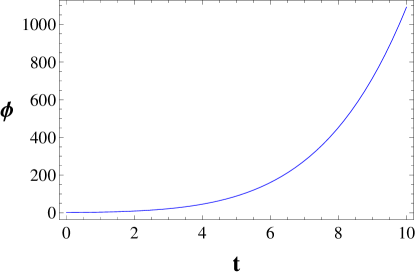
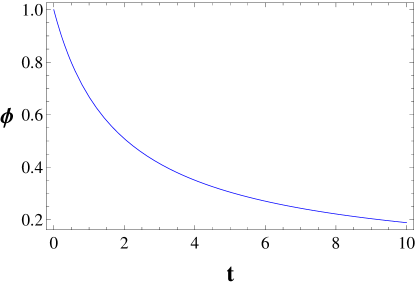
Figure 1: The time behavior of the BD scalar field corresponding to slow (upper panel) and fast (lower panel) solutions. We have taken $a_{0}=1=\phi_{0}$, $c_{2}=-1$, $\theta=0$ and $\omega=-1.2$. Note that these curves, unlike their corresponding $a(t)$ curves [associated to both of the commutative and noncommutative (with small values of the $\theta$) cases] coincide.

It has been shown V91-GV92-TV92-GPR94 that when $\omega\neq-4/3$, by redefining $\Phi\equiv-{\rm ln}(G\phi)$ (where $G$ is the gravitational constant), there are duality transformations as

$$\alpha \rightarrow \left(\frac{3\omega+2}{3\omega+4}\right)\alpha-2\left(\frac{\omega+1}{3\omega+4}\right)\Phi,$$ (25)

$$\Phi \rightarrow -\left(\frac{6}{3\omega+4}\right)\alpha-\left(\frac{3\omega+2}{3\omega+4}\right)\Phi,$$

under which the slow and fast solutions are interchanged L95-L96 , namely, $(r_{\pm},s_{\pm})\longleftrightarrow(r_{\mp},s_{\mp})$. However, in our model for $\theta=0$ herein, from general relations (24), without considering the duality transformations (25), we can see that the sign of the integration constant $c_{2}$ is responsible for the mentioned role, interchanging the lower-upper solutions. More precisely, under interchanging $c_{2}>0\leftrightarrow c_{2}<0$, the parameters $c_{1}$, $g$, and $f$ transform as $(c_{1}^{\pm},f^{\pm},g^{\pm})\longleftrightarrow(-c_{1}^{\mp},-f^{\mp},g^{\mp})$, and, consequently, we get $(r_{\pm},s_{\pm})\longleftrightarrow(r_{\mp},s_{\mp})$. By considering such a symmetry, a relevant counterpart between the solutions can be made, such that the number of different cases to study are reduced by half. We also notice that, for the noncommutative case where $\theta\neq 0$, as seen from (13), the general duality transformations (if one can find them), not only depend on the $f$, $g$, and the integration constants $c_{1}$ and $c_{2}$ but also may depend on the noncommutativity parameter.

In the rest of this section, we will investigate the results of a few numerical solutions for the noncommutative case which will be compared with the corresponding solutions of the commutative case.

III.1 Case I: The lower sign with $c_{2}>0$, $\omega<0$

In the commutative case, for $c_{2}>0$, $\omega<0$, and the lower sign, the time behavior of the scalar field and scale factor depend on the values of the $\omega$, in which, when $\omega$ is restricted to $-3/2<\omega<-4/3$, the scalar field decreases while the scale factor always accelerates. However, for $-4/3<\omega<0$, we observe a different behavior for the scalar field and scale factor, such that, for this case, the former increases but the latter decreases. For this, in Fig. 2, according to the relations (24), we have plotted the behaviors of the exponents $r_{-}$ and $s_{-}$ versus $\omega$ in the range $-3/2<\omega<0$. Hence, in order to have a simple comparison of the commutative and noncommutative cases, perhaps it will be a good idea if we also investigate these ranges of $\omega$ in separate parts for the commutative and noncommutative cases. As the behavior of the quantities is sensitive to the sign of the noncommutative parameter, we will investigate various cases for positive and negative $\theta$.

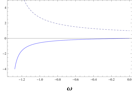
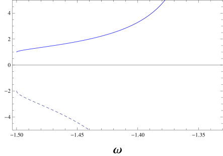
Figure 2: The behavior of the exponents $r_{-}$ (solid curves) and $s_{-}$ (dashed curves) versus $\omega$ associated to the commutative case for the lower sign when $c_{2}>0$. We have chosen the ranges $-4/3<\omega<0$ and $-3/2<\omega<-4/3$ for the upper and lower panels, respectively.

III.1.1 Case Ia: $-3/2<\omega<-4/3$ and $\theta<0$

In order to compare the behavior of the quantities, in Figs. 3 and 4, we have plotted the time behavior of the scalar field, scale factor, and its first and second time derivatives for the commutative and noncommutative cases, respectively. In these plots, except for the noncommutative parameter, we have chosen the same initial values for the variables: very small negative values for the noncommutative parameter and negative values for the BD parameter in the range $-3/2<\omega<-4/3$ and $a_{0}=\phi_{0}=c_{2}=1$. We should remind that, in order to probe the effects of the noncommutative parameter with more clarity, Figs. 3 and 4 have been plotted separately for each case.

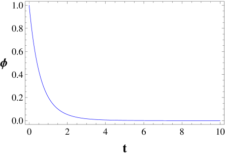
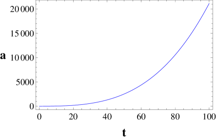
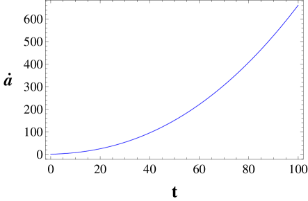
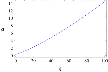
Figure 3: The time behavior of the BD scalar field, scale factor, its first and second derivatives associated to the commutative case ($\theta=0$) for the lower sign with $a_{0}=\phi_{0}=c_{2}=1$ and $\omega=-1.4$.

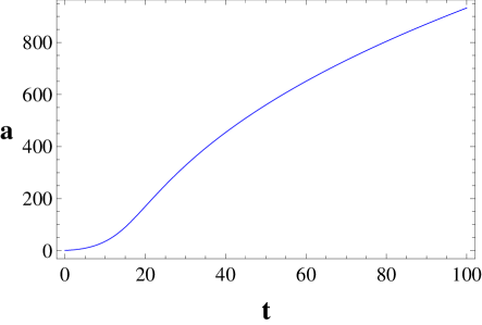
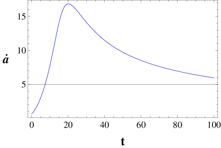
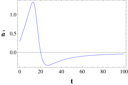
Figure 4: The time behavior of the scale factor, its first and second derivatives associated to the noncommutative case for the lower sign. We have taken $\theta=-0.000001$. All the other initial values are the same as they were in Fig. 3. Note that the $\phi(t)$ curves associated to the commutative and noncommutative cases almost coincide.

As Figs. 3 and 4 show, the scalar field decreases, and its behavior is almost the same for both of the commutative and noncommutative cases (they almost coincide). However, the behavior of the scale factor is different. That is, the scale factor starts from a singular point at $t=0$ and increases for both of the commutative and noncommutative cases, such that, for the commutative case, we always have $\ddot{a}>0$, while for the noncommutative case in the early times we have $\ddot{a}>0$, but at the special point (hereafter, we call it “point A”), it turns to be negative; namely, after a very small time, the phase changes and we have a decelerating universe. In the next sections, we will discuss further such an interesting behavior of the scale factor. It is worthwhile to describe the evolution of the scale factor, scalar field and their time derivatives for different values of the three present parameters in this case. Namely, for different values which have been chosen from the ranges $c_{2}>0$, $\theta<0$, and $\omega<0$. The results indicate the following:

• The larger the integration constant $c_{2}$, the shorter the time of the accelerating phase (see Fig. 5). Namely, when we take a larger $c_{2}$, the scale factor increases faster (with a larger speed and acceleration), and, consequently, we get to the point A faster. In other words, by increasing this integration constant, the $\ddot{a}$ curve is shifted to the left simultaneously with a contraction of the amount of the time associated to the accelerating (as well as decelerating) and an increase of $|\ddot{a}|$ for both the accelerating and decelerating phases. Furthermore, as Fig. 5 demonstrates, by taking a larger value for $c_{2}$, the scalar field decreases faster. Consequently, as the value of $c_{2}$ determines the time of the accelerating phase and its corresponding scale factor value, it can, thus, be related to the number of $e$-folds for an inflationary universe.

  

  

  

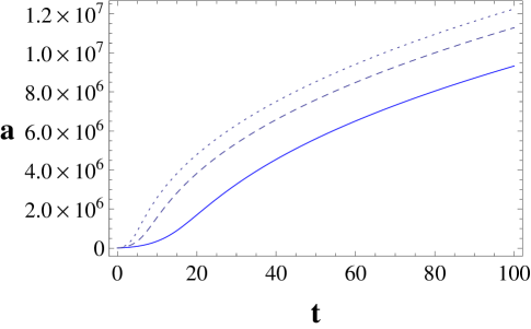
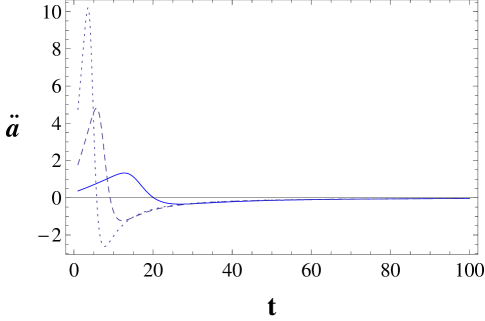
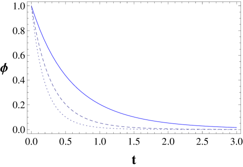
  Figure 5: The time behavior of the $a$, $\ddot{a}$ and the $\phi$ for the noncommutative case with different $c_{2}$. In this figure, we take three different values as $c_{2}=1$ (solid curve), $c_{2}=2$ (dashed curve) and $c_{2}=3$ (dotted curve). The other parameters have the same initial values as in Fig. 3

• In Fig. 6, we have plotted the behavior of the scale factor and its derivatives (with respect to the cosmic time) for different values of the noncommutative parameter. For different values of $\mid\!\theta\!\mid$, we cannot see perceptible changes in the behavior of the scalar field. However, the smaller the $\mid\!\theta\!\mid$, the larger the slope of $a(t)$, namely $\dot{a}$. More precisely, the speed of the expansion directly depends on the $\mid\!\theta\!\mid$. More concretely, the time behavior of $a$ (and, consequently, $\dot{a}$ and $\ddot{a}$), by taking different values of the noncommutative parameter, changes, such that as Figs. 5 and 6 show, it seems that $\mid\!\theta\!\mid$ plays the role of $c_{2}^{-1}$ (as the previous item shows) in the $\ddot{a}$ plots. This claim is true for the amount of the interval time of the accelerating and decelerating phases, but it does not hold for the value of $\mid\!\ddot{a}\!\mid$, because in this case, the larger the value of $\mid\!\theta\!\mid$, the smaller the value of $\mid\!\ddot{a}\!\mid$. Hence, we should note that, as the numerical results show, it is not valid to argue that when the value $\mid\!c_{2}\theta\!\mid$ remains constant, the behavior of the scalar field, scale factor, and their time derivatives do not change. This can be read from (20) and (21); namely, the extra role of $c_{2}$ in other parts of the differential equations, for instance, the $f$ itself, depends on $c_{2}$ rather than $\theta$.

  

  

  

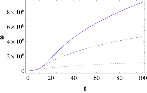
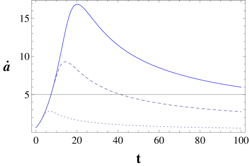
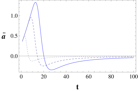
  Figure 6: The time behavior of the $a$, $\dot{a}$ and $\ddot{a}$ for the noncommutative case for different values of the noncommutative parameter. Here, we take $c_{2}=1=a_{0}$, $\omega=-1.4$ for three different values of the noncommutative parameter as $\theta=-0.000001$ (solid curve), $\theta=-0.00001$ (dashed curve) and $\theta=-0.001$ (dotted curve).

• For large values of the cosmic time, by assuming the same initial values for the parameters of the model (except $\theta$), the BD scalar field goes to zero for both the commutative and noncommutative cases. However, the time behavior of the scale factor is not the same for these cases. In the commutative case, the scale factor always accelerates with a variable acceleration, such that $\ddot{a}$ never takes a constant value. However, for the noncommutative case, $\ddot{a}$ vanishes, $\dot{a}$ takes very small constant value, and, consequently, the Universe expands with a small constant speed. Namely, in the noncommutative case, for late times, we get a zero acceleration epoch. Such behavior for the scale factor can be interpreted as a direct consequence of the existence of the noncommutative parameter. This is almost similar to the result obtained in RFK11 , in which a constant deformation parameter is also included. However, the difference is that, in our model, the speed of the scale factor in late times is not exactly zero, but it approaches zero instead. We should note that in RFK11 , as the behavior of the quantities were investigated, when $\omega\longrightarrow\infty$, such a difference can be interpreted as a natural consequence of the models. This effect of the noncommutative parameter shows itself very far from the initial singularity, and it has been suggested as a footprint of quantum gravity in a coarse-grained explanation.

III.1.2 Case Ib: $-4/3<\omega<0$ and $\theta<0$:

As mentioned, in this range of the BD coupling parameter, for the commutative case, our solutions are more general than the solutions obtained by O’Hanlon and Tupper. More precisely, in the O’Hanlon-Tupper solutions, for the lower sign with $-4/3<\omega<0$, the BD scalar field always increases while the scale factor decreases. However, the behavior of these quantities in our model not only depends on the values of $\omega$ but is also sensitive to the values of the integration constant $c_{2}$, such that by taking different values for $\omega$ and $c_{2}$, we can obtain, in addition to the O’Hanlon-Tupper solutions other different behaviors as obtained in case Ia. For instance, in Fig. 7, we have plotted the behavior of the BD scalar field for two different values of $c_{2}$. Note that the other initial values are the same for both of these figures. Moreover, for the noncommutative case, we also observe that the behavior of these quantities depends on, besides $c_{2}$ and $\omega$, the noncommutative parameter. In short, for the noncommutative case, the obtained solutions in the previous case (case Ia) can also be produced when we take the range $-4/3<\omega<0$, although the initial values may be changed.

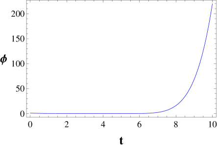
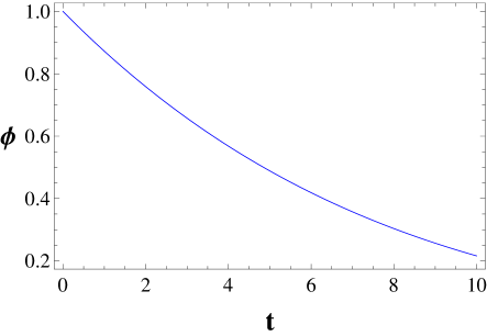
Figure 7: The time behavior of the BD scalar field for the commutative case for different values for $c_{2}$ as $c_{2}=1$ (upper panel) and $c_{2}=0.1$ (lower panel). The other initial values have been taken the same for both of the plots. Here, $a_{0}=1$, $\omega=-1.2$ and $\theta=0$.

III.2 Other cases

We can also add a new case, i.e., the lower sign in which $c_{2}>0$, $\omega<0$, and $\theta>0$, instead of negative values for the noncommutative parameter. Also, we can analyze other cases similar to those categorized in case I but instead with an upper sign (rather than a lower sign). However, as all of the mentioned cases give different results, which are not in the scope of this work, we will leave them.

IV Kinetic inflation

In the previous section, we have shown that by introducing a noncommutative relation between the BD scalar field and the logarithm of the scale factor, not only does the scale factor accelerate in the early times, but also it can exit from the acceleration epoch and initiate a decelerating phase. In other words, a suggestion on how to solve the graceful exit problem. However, these features alone do not guarantee an appropriate setting for the resolution of the problems with the standard cosmology.

One of the well-known shortcomings with the standard cosmology is the horizon problem. Namely, there are plenty of regions in the large volume of today’s Universe, which were not causally connected at early times. More precisely, the size of the presently observed Universe at some earlier time $t$ (at least as early as $t\sim 1sec$), $d_{{}_{\rm U}}(t)\sim a(t)/(H_{0}a_{0})$, is much larger than a distance which a photon traveling by $t$, $d^{{}^{\rm Hor}}(t)=a(t)\int_{t_{i}}^{t}dt^{\prime}/a^{\prime}$ [28]. Let us first check the nominal condition for the acceleration associated to the inflation Lev95 , namely,

$$d^{{}^{\rm Hor}}>H^{-1}.$$ (26)

Then, in the rest of this section, we will investigate the condition for sufficient inflation.

From Eqs. (12) and (13), we get

$$\left(H+\frac{\dot{\phi}}{2\phi}\right)^{2}=\left[\left(h+\frac{1}{2}\right)\left(\frac{\dot{\phi}}{\phi}\right)\right]^{2},$$ (27)

which gives

$$\frac{d{\rm ln}(a^{2}\phi)}{dt}=\pm(2h+1)\left(\frac{\dot{\phi}}{\phi}\right).$$ (28)

This equation shows that the horizon distance can be related to $\phi$, $\omega$, the scale factor, and the noncommutatvity parameter. Applying (12) and integrating over $dt$, we obtain

$$d^{{}^{\rm Hor}}=\frac{a^{3}\phi}{|f|}-\frac{2c_{2}}{2g+1}d^{{}^{\rm NC}}$$ (29)

up to a constant of integration. In Eq. (29), we have introduced the new distance $d^{{}^{\rm NC}}$ as

$$d^{{}^{\rm NC}}\equiv\frac{\theta a}{c_{2}}\int\frac{P^{\prime}_{\phi^{\prime}}dt^{\prime}}{a^{\prime}},$$ (30)

in which the integrand not only depends on the inverse of the scale factor (similar to the one defined for optical horizon) but also depends on the nonocommutativity parameter and the conjugate momentum of the BD scalar field. The factor $c_{2}$ is multiplied in the denominator of relation (30) to make the dimension of $d^{{}^{\rm NC}}$ the same as $d^{{}^{\rm Hor}}$. (Note that we have found a relation between the BD scalar field and its momentum conjugate as $P_{\phi}=c_{2}/\phi$.) We expect that this new term can add a positive value to the $d^{{}^{\rm Hor}}$ to properly assist in satisfying the requirement associated to the horizon problem. In order to compare, we rewrite Eq. (13) by the aid of (12) as

$$H=\frac{|f|}{\xi}\frac{h}{a^{3}\phi}.$$ (31)

Using (29) and (31) in the nominal condition (26) gives

$$D^{{}^{\rm NC}}\equiv d^{{}^{\rm Hor}}\!\!-H^{-1}=\frac{\phi a^{3}}{|f|}\left(\!\!1+\frac{\xi}{h}\right)-\frac{2d^{{}^{\rm NC}}}{2g+1}>0.$$ (32)

Obviously, in the limit $\theta\longrightarrow 0$, $d^{{}^{\rm NC}}$ goes to zero as well, and, thus, the relation associated to the horizon distance of the commutative case is recovered. Further, in the mentioned limit, the resulted relation is the same as one obtained in Ref. Lev95 (by assuming a constant BD coupling parameter in the mentioned paper). Therefore, in the commutative case where $\theta=0$, the only acceptable result is $0<\xi<1$ ($-3/2<\omega<0$), which is obtained by choosing either the upper sign for $c_{2}>0$ or the lower sign for $c_{2}<0$.

For the general noncommutative case, we should note that, in addition to the sign of $c_{2}$, the allowed values of $\omega$ as well as the behavior of the BD scalar, the noncommutative parameter has a substantial role in determining whether this constraint is satisfied or not. Obviously, as the numerical results of the previous section show (see, especially, Figs. 5 and 6 and their analysis), due to the presence of the noncommutative parameter and the extra terms associated to it, satisfying the constraints for the noncommutative case is easier than its corresponding commutative case. For instance, in Fig. 8, for case Ia, $D^{{}^{\rm NC}}$ has been plotted against cosmic time. Therefore, we observe that the constraint (32) for the noncommutative case can be easily satisfied at all times. To be more clear, we also have plotted the time behavior of $D^{{}^{\rm NC}}$ for the commutative case ($\theta=0$) separately in Fig. 9.

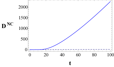
Figure 8: The time behavior of the $D^{{}^{\rm NC}}$, the quantity which defined as in (32). The solid and dashed curves are associated to the noncommutative and commutative cases, respectively. This figure is prepared as an example to indicate that the nominal condition (26) for the noncommutative solutions (specially for the case Ia) can be easily satisfied. The initial values are $a_{0}=1=c_{2}$, $\omega=-1.4$, $\theta=-0.000001$ (solid curve) and $\theta=0$ (dashed curve).

Figure 9: The time behavior of the $D^{{}^{\rm NC}}$ for the commutative case with the same initial values as in Fig. 8.

In what follows, we intend to probe the condition for sufficient inflation, which is given by Lev95-2

$$\frac{{d}^{{}^{\rm Hor}}_{\star}}{a_{\star}}>\frac{1}{H_{0}a_{0}},$$ (33)

where the lhs of the above inequality stands for a comoving size of a causally connected region at a specific earlier time $t_{\star}$. By including a nonzero integration constant, relation (28) for the specific time $t_{\star}$ gives

$$d^{{}^{\rm Hor}}_{\star}=\frac{a^{3}\phi(1-\delta)}{f{\rm sgn}(c_{2})}-\frac{2}{2g+1}d^{{}^{\rm NC}}\Biggr{|}_{\star},$$ (34)

where the integration constant, which was removed in relation (29), has now been included in $\delta\equiv\frac{a_{i}^{2}\phi_{i}}{a^{2}\phi}$ where the subscript $i$ stands for initial values. Note that, as the BD scalar field takes positive values, we always have $\delta\geq 0$.

The Hubble constant at present time, $H_{0}$, can be expressed in terms of the value of the Planck mass today, $M_{0}$, and $T_{0}$ as Lev95-2

$$H_{0}=\sqrt{\hat{\alpha}_{0}}\frac{T_{0}^{2}}{M_{0}},$$ (35)

where $\hat{\alpha}_{0}=\gamma(t_{0})\eta_{0}=(8\pi/3)(\pi^{2}/30)\bar{g}(t_{0})\eta_{0}$, in which $\eta_{0}$ stands for the ratio today of the energy density in matter to that in radiation. In order to see whether or not the above condition is satisfied by the solutions herein, we would like to employ the assumptions of the Ref. Lev95-2 : (i) the time $t_{\rm end}$ is allocated to the end of inflation in which the entropy is produced; (ii) since the time $t_{\rm end}$, the Universe has evolved adiabatically such that we can assume $a_{\rm end}T_{\rm end}=a_{0}T_{0}$. Employing relation (35) and assumption (ii) in (33) gives

$$\frac{a_{\star}}{a_{\rm end}}\gtrsim\left(\frac{M_{0}}{\sqrt{\bar{\alpha}_{0}}T_{0}}\right)\frac{1}{\mid\!\!d^{{}^{\rm Hor}}_{\star}\!\!\mid T_{\rm end}}.$$ (36)

In order to proceed, we consider a simple conjecture for the heating mechanism. Let us use the following relation between $T_{\rm end}$ and the net available kinetic energy $E_{\rm end}$ as

$$T_{\rm end}=\epsilon E_{\rm end},$$ (37)

where $\epsilon$ denotes the efficiency of the system where the kinetic energy density is converted to entropy Lev95-2 . The kinetic energy density for our model is only given by the energy density of the BD scalar field in unit volume. Namely, we have $E_{\rm end}=\rho^{(\phi)}_{\rm end}(4\pi/3)a^{3}_{\rm end}$, where by substituting the energy density associated to the BD scalar field from relation (16), we obtain

$$T_{\rm end}=\frac{4\pi\epsilon f^{2}}{\xi^{2}}\frac{h^{2}_{\rm end}}{a^{3}_{\rm end}\phi_{\rm end}}.$$ (38)

Substituting $d^{{}^{\rm Hor}}_{\star}$ from (34) and $T_{\rm end}$ from (38) into (36), we get

$$\frac{a_{\star}^{2}\phi_{\star}}{a_{\rm end}^{2}\phi_{\rm end}} \gtrsim \left(\frac{M_{0}}{\sqrt{\bar{\alpha}_{0}}T_{0}}\right)(1-\delta_{\star})^{-1}\xi^{2}$$

$$\times \frac{1}{4\pi\epsilon\mid f\mid(g+\frac{c_{2}\theta}{\phi})^{2}[1-\frac{2d^{{}^{\rm NC}}_{\star}}{(2g+1)\mid f\mid(1-\delta_{\star})a_{\star}^{3}\phi_{\star}}]}.$$

The constraint (IV) is the modified (noncommutative) version of the one obtained in the BD theory in Lev95-2 .

Let us first review the obstacles of the commutative model regarding (33) and then turn to solve the problems by applying the noncommutative model. In Lev95-2 , $(1-\delta_{\star})\sim 1$, $f\sim 1$, $M_{0}=1.2\times 10^{19}{\rm GeV}$, $T_{0}=2.3\times 10^{-13}{\rm GeV}$, and assigning two different values for $\omega$, the model was examined. In one case where $\omega\sim 0$, satisfying (4.8) leads us to take the D branch. Let us be more precise. By substituting the above values in the inequality for the commutative case, the constraint $(a_{\star}^{2}\phi_{\star})/(a_{\rm end}^{2}\phi_{\rm end})\gtrsim 10^{30}/\epsilon$ follows. This condition, even with $\epsilon\sim 1$, implies that the quantity $a^{2}\phi$ decreases with the cosmic time. Such a result demands that we must take the D branch of the solutions. However, to have an expanding universe, we must have $a_{\rm end}>a_{\star}$. By using this requirement in (IV) for the commutative case, the minimum change in the dynamical Planck mass will be  $m_{\rm Pl}(t_{\rm end})/m_{\rm Pl}(t_{\star})\gtrsim 10^{-15}\epsilon^{1/2}$, which implies that the Planck mass must decrease during inflation. However, as was argued by Levin Lev95-2 , it is not enough that such a requirement is satisfied, and a branch change must be induced.

Let us further discuss the assistance of a few plots from our model for the lower sign with $c_{2}>0$ (D branch) and then compare it with the noncommutative case. Equation (28), by using (13) and (14) for the lower sign, can be rewritten as

$$\frac{d{\rm ln}(a\phi^{\frac{1}{2}})}{dt}=-\frac{1}{2}\Big{[}{\rm sgn}(c_{2})\xi+\frac{2c_{2}\theta}{\phi}\Big{]}\left(\frac{|f|}{\xi a^{3}\phi}\right).$$ (40)

In the commutative case with $c_{2}>0$, we get

$$\frac{d{\rm ln}(a\phi^{\frac{1}{2}})}{dt}=-\frac{|f|}{2a^{3}\phi},$$ (41)

which indicates that the quantity $a\phi^{1/2}$ always decreases with the cosmic time. In Fig. 10, such behavior has been shown for the lower sign (see the dashed curve).

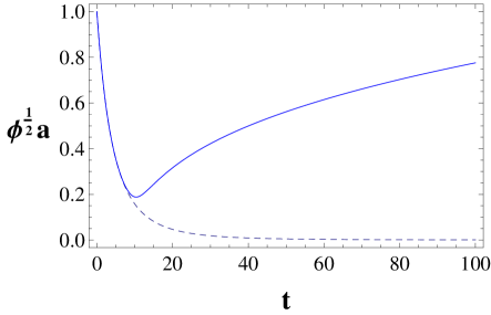
Figure 10: The time behavior of the $a\phi^{1/2}$ for the commutative case (dashed curve) and noncommutative case (solid curve). We have taken $c_{2}=1=a_{0}$, $\omega=-1.36$ and $\theta=-0.000001$ for the noncommutative case.

Because a variation in the strength of gravity for today’s Universe has not been observed, this behavior is consequently not acceptable: namely, the BD scalar field must take almost constant values today. On the other hand, as we have an expanding universe, the quantity $a\phi^{1/2}$ has to increase. While for a general noncommutative case, due to the complicated dependence of the rhs of (40) to $c_{2}$, $\omega$, $\theta$, as well as the BD scalar field, we cannot analytically draw the time behavior of $a\phi^{1/2}$. However, fortunately, for $c_{2}>0$, $\theta<0$, and lower case, i.e., the D branch, we have shown numerically that at the early times, $a\phi^{1/2}$ behaves the same as its corresponding in the commutative case; namely, it decreases with time. However, after reaching a nonzero minimum, it starts to increase. For instance, in Fig. 10, the time behavior of $a\phi^{1/2}$ for the lower sign associated to the noncommutative case has been plotted.

We also should remind that in the commutative case, even with taking a variable BD coupling parameter, the D branch cannot give today’s expanding Universe. Hence, such a result is not consistent with the present accelerating Universe.

V conclusions

In this paper, we have introduced a noncommutative version of the BD theory. More precisely, a modified Poisson algebra among minisuperspace variables (the logarithm of the scale factor and the BD scalar field) has been used. Such an ansatz bears much resemblance to the assumptions taken in noncommutative quantum cosmology GOR02 ; BP04-PM05-AAOSS07-GSS07 as well as a few classical noncommutative cosmological models in theories alternative to general relativity with a minimally GSS11 ; RZMM14 (or a nonminimally RFK11 ) coupled scalar field to the geometry.

We have investigated the BD cosmological equations of motion in the comoving gauge. The general Hamiltonian equations indicate that when the noncommutative parameter tends to zero, all the equations reduced to their corresponding counterparts in the standard commutative case.

We have focused on the case in which there is neither a scalar potential nor a cosmological constant. Furthermore, we have assumed that the Lagrangian density associated to the ordinary matter is absent. We constructed a generalized noncommutative analogue to include key ideas of duality and branch changing as well as gravity-driven acceleration and kinetic inflation. In this manner, we have seen that the power-law scale factor of the Universe (associated to the commutative case) is generalized to be multiplied with a time-dependent exponential warp factor, which is a function of the noncommutative parameter and the momentum associated to the BD scalar field [see relation (20)]. Moreover, in this case, in contrast to the commutative case, we have observed that the BD scalar field is not in the form of a simple power function of time, but instead, it is obtained from a more complicated differential equation, which is found to be an incomplete gamma function [see differential equation (21)].

In the commutative case, because of the appearance of the integration constant associated to the momentum conjugate of the BD scalar field in the solutions, our model can be considered as an extended model of the de Sitter–like space and O’Hanlon-Tupper solutions. In the latter, the mentioned integration constant has an interesting property. Namely, under changing its sign, a symmetry relates a category of the solutions to its corresponding counterpart, such that the number of models to be discussed can be reduced by half. More precisely, this integration constant together with others presented in the model can play the role of the duality transformations introduced in the context of the BD theory L95-L96 .

After a short discussion of the consequences of our model within the standard commutative case, we have focused on noncommutative solutions (and their interesting interpretations in cosmology), which give very different results with respect to their corresponding in the commutative case.

In case Ia, we have assumed very small negative values of the noncommutative parameter $\theta$, positive values of $c_{2}$, and the lower sign. We have shown that, unlike the time behavior of the BD scalar field, the time behaviors of the scale factor, its speed, and acceleration are very different in the noncommutative case with respect to the commutative case. Let us be more concrete. When the BD coupling parameter is restricted to $-3/2<\omega<0$, the scale factor of the commutative case always accelerates, while, for the noncommutative case, it accelerates only for the very early times, and after a very short time, it turns to give a decelerated universe. This interesting effect of the noncommutative parameter on the behavior of the scale factor constitutes a feature of an appropriate alternative model proposed for an inflationary model, which can overcome the graceful exit problem.

Furthermore, the mentioned behavior of the scale factor can also be altered with different allowed values of the parameters present in the model. More precisely, when different values are taken for $\theta$, $\omega$, and $c_{2}$, the time interval, speed, and acceleration of the scale factor associated to the acceleration phase of the very early era of the universe also change. We have numerically shown that the $e$-folding number relates to the amount of $c_{2}$ and/or $\theta$. Our numerical analysis show that, for case Ia, the noncommutative minisuperspace model, in which the noncommutative parameter is a constant, can constitute as a viable phenomenological model herein, at least for an inflationary epoch, when $\mid\theta\mid$ takes very small values.

Moreover, in case Ia for late times, contrary to the commutative model in which the scale factor always accelerates, we get a zero acceleration epoch for the Universe. This behavior of the scale factor that is occurring very far from the singularity is guaranteed by the existence of a constant noncommutative parameter, and it is usually interpreted as coarse-grained explanation of the quantum gravity footprint.

The horizon problem is the main shortcoming with the standard cosmology, so, we turned to investigate it in our model. We have shown that by extending the FLRW vacuum universe, in the standard BD theory, by introducing a deformation among the minisuperspace variables, we can overcome this problem.

By means of numerical diagrams, we have shown that the nominal as well as sufficient requirements associated to the inflation can be fully satisfied in our model. In a kinetic inflation model in the context of the BD theory with a variable $\omega$ for the commutative case Lev95-2 , it was claimed that all the accelerations in the D branch suffer from the well-known graceful exit problem. Namely, such a problem has a direct relation with the time behavior of the quantity $a\phi^{1/2}$. More precisely, if $a\phi^{1/2}$ decreases forever, then a branch change is required. Indeed, in the commutative case, the mentioned quantity always decreases which is in direct contradiction with the observational indications concerning the strength of the gravity as well as the expansion of today’s Universe. This problem is properly solved by the effects of the noncommutative parameter, such that at the very early times, exactly the same as the commutative case, $a\phi^{1/2}$ decreases with the cosmic time, while after the phase changing, it starts to increase with time, which is in agreement with observation.

Let us look at the above problem from another perspective. If we would like to know whether or not the model also provides inflation in the conformal Einstein frame, we must consider not only the behavior of the scale factor but also check the behavior of the quantity $a_{{}_{\rm RI}}\equiv[a(t)l_{0}]/l_{\rm Pl(t)}$, in which $a(t)l_{0}$ (where $l_{0}$ is a comoving constant length) is any physical length, and $l_{\rm Pl}(t)\equiv\sqrt{\frac{\hbar G_{\rm eff}}{c^{3}}}=\sqrt{\frac{\hbar}{c^{3}\phi(t)}}$ is the Planck length, which is not a constant in BD theory. If the mentioned conditions were satisfied, then inflation is called real inflation Faraoni.book . As mentioned, in some models, the Planck length decreases faster than the scale factor, and, thus, the ratio $a_{{}_{\rm RI}}$ always decreases, which is not consistent with the observational data. However, in our model, as we have used the Planck units, the ratio $a_{{}_{\rm RI}}$ reduces to the quantity $a\phi^{1/2}$, and, thus, our model provides real inflation. However, in the case of the commutative model, for any $\omega$, particularly for the case $\omega=-1$, which has been known as pre-big-bang cosmology LWC00 , the requirements of the real inflation are not fully satisfied C98 ; C99 .

We should be aware of some shortcomings regarding our noncommutative setting herein.

• In our model, as in other investigations in the context of the BD theory, to retrieve the acceleration for the early as well as late time epochs, the BD coupling parameter takes very small values, which is in contradiction with Solar System experiments. Different approaches have been presented to solve the shortcomings with the cosmological models based on the BD theory, especially the mentioned problem with $\omega$, see, e.g., Refs. BM90 ; LSB89-PSW08-WW12 .

• In this paper, we have confined our discussion to the noncommutative version of the standard BD theory in the absence of the ordinary matter, but we can extend this procedure by adding a matter sector, scalar potential, and/or assuming a variable BD coupling parameter instead of the constant one. In addition, we can consider other deformed Poisson brackets instead of the one presented here.
  

• Another important point is that we have not tested the predictions of our model (for the very early Universe) by means of density and gravitational fluctuations around the FLRW background. In many investigations, by employing different approaches, the perturbation of the FLRW background in the BD and generalized scalar-tensor theories have been studied, see, e.g., Faraoni.book ; HN96-BFG96-M09-CDG13 . Employing perturbation theory, similar to transformations required for finding the predictions of the model in the conformal Einstein frame, is crucial, but performing them in the presence of the noncommutative parameter is very complicated and in some situations may be impossible.

VI ACKNOWLEDGMENTS

S. M. M. Rasouli is grateful for the support of Grant No. SFRH/BPD/82479/2011 from the Portuguese Agency Fundação para a Ciência e Tecnologia. This research work was supported by Grants No. CERN/FP/123618/2011 and No. PEst-OE/MAT/UI0212/2014.

References

- (1) C. Brans and R.H. Dicke, Phys. Rev. 124, 925 (1961).
- (2) V. Faraoni, Cosmology in Scalar Tensor Gravity (Kluwer Academic, Dordrecht, 2004).
- (3) N. Banerjee and D. Pavon, Phys. Rev. D 63, 043504 (2001).
- (4) A.E. Montenegro, Jr. and S. Carneiro, Classical Quantum Gravity 24, 313 (2007).
- (5) S.M. M. Rasouli, M. Farhoudi and P. V. Moniz, Classical Quantum Gravity 31, 115002 (2014).
- (6) S.M. M. Rasouli, M. Farhoudi and H. R. Sepangi, Classical Quantum Gravity 28, 155004 (2011); S. M. M. Rasouli, Prog. Math. Rel., Gravit. Cosmol. 60, 371 (2014).
- (7) D. La and P. J. Steinhardt, Phys. Rev. Lett. 62, 376 (1989); P. J. Steinhardt and F. S. Accetta, Phys. Rev. Lett. 64, 2740 (1990); S. Capozziello and M. De Laurentis, Phys. Rep. 509, 167 (2011); T. Clifton, P. G. Ferreira, A. Padilla and C. Skordis, Phys. Rep. 513, 1 (2012).
- (8) J. D. Barrow and K. Maeda, Nucl. Phys. B341, 249 (1990).
- (9) J. J. Levin, Phys. Rev. D 51, 462 (1995).
- (10) J. J. Levin, Phys. Rev. D 51, 1536 (1995).
- (11) R. Brustein and G. Veneziano, Phys. Lett. B 329, 429 (1994).
- (12) A. Connes, M. R. Douglas and A. Schwarz, J. High Energy Phys. 09, (1998) 003; M. R. Douglas and N. A. Nekrasov, Rev. Mod. Phys. 73, 977 (2001); N. Seiberg and E. Witten, J. High Energy Phys. 09, (1999) 032.
- (13) H. Garcia-Compean, O. Obregon, C. Ramirez and M. Sabido, Phys. Rev. D 68, 044015 (2003); H.Garcia-Compean,O. Obregon,C.Ramirez and M.Sabido, Phys. Rev. D 68, 045010 (2003); P. Aschieri, M. Dimitrijevic, F. Meyer and J. Wess, Classical Quantum Gravity 23, 1883 (2006); S. Estrada-Jimenez, H. Garcia-Compean, O. Obregon and C. Ramirez, Phys. Rev. D 78, 124008 (2008).
- (14) G.D. Barbosa and N. Pinto-Neto, Phys. Rev. D 70, 103512 (2004); L. O. Pimentel and C. Mora, Gen. Relativ. Gravit. 37, 817 (2005); M. Aguero, J. A. Aguilar, S. C. Ortiz, M. Sabido and J. Socorro, Int. J. Theor. Phys. 46, 2928 (2007); W. Guzman, M. Sabido and J. Socorro, Phys. Rev. D 76, 087302 (2007).
- (15) S. M. M. Rasouli, M. Farhoudi and N. Khosravi, Gen. Rel. Grav. 43, 2895 (2011).
- (16) S. M. M. Rasouli, A. H. Ziaie, J. Marto, and P. V. Moniz Phys. Rev. D 89 044028 (2014).
- (17) W. Guzmán, M. Sabido and J. Socorro, Phys. Lett. B 697, 271 (2011).
- (18) V. Faraoni, Classical Quantum Gravity 26, 145014 (2009).
- (19) P. Jordan, Projective Relativity (Friedrich Vieweg und Sohn, Braunschweig, 1955); V. Faraoni, E. Gunzig and P. Nardone, Fundam. Cosm. Phys. 20, 121 (1999).
- (20) D. H. Coule, Classical Quantum Gravity 15, 2803 (1998).
- (21) J.D. Barrow, D. Kimberly and J. Magueijo, Classical Quantum Gravity 21, 4289 (2004); M.P. Dabrowski, T. Denkiewicz and D. Blaschke, Ann. Phys. (Amsterdam) 16, 237 (2007); K.A. Bronnikov and A.A. Starobinsky, JETP Lett. 85, 1 (2007); P. Bonifacio, Ph.D. thesis, University of Aberdeen, 2009, arXive: gr-qc/0906.0463.
- (22) H. Garcia-Compean, O. Obregon and C. Ramirez, Phys. Rev. Lett. 88, 161301 (2002).
- (23) J. E. Lidsey, Phys. Rev. D 55, 3303 (1997).
- (24) J. O’Hanlon and B.O.J. Tupper, Nuovo Cimento Soc. Ital. Fis. 7B, 305 (1972); S.J. Kolitch, and D.M. Eardley, Ann. Phys. (N.Y.) 241, 128 (1995); J.P. Mimoso and D. Wands, Phys. Rev. D 51, 477 (1995).
- (25) G. Veneziano, Phys. Lett. B 265, 287 (1991); M. Gasperini and G. Veneziano, Phys. Lett. B 277, 256 (1992); A. A. Tseytlin and C. Vafa, Nucl. Phys. B 372, 443 (1992); A. Giveon, M. Porrati, and E. Rabinovici, Phys. Rep. 244, 77 (1994).
- (26) J. E. Lidsey, Phys. Rev. D 52, R5407 (1995); Classical Quantum Gravity 13, 2449 (1996).
- (27) V. Faraoni, Phys. Rev. D 84, 024003 (2011).
- (28) Y. Hu, M. S. Turner and E. J. Weinberg, Phys. Rev. D 49, 3830 (1994).
- (29) J. J. Levin and K. Freese, Nucl. Phys. B421, 635 (1994).
- (30) H. Garcia-Compean, O. Obregon and C. Ramirez, Phys. Rev. Lett. 88, 161301 (2002).
- (31) J. E. Lidsey, D. Wands and E. J. Copeland, Phys. Rep. 337, 343 (2000).
- (32) D. H. Coule, Phys. Lett. B 450, 48 (1999).
- (33) D. La, P. J. Steinhardt and E. Bertschinger, Phys. Lett. B 231, 231 (1989); R. Punzi, F. P. Schuller and M. N. R. Wohlfarth, Phys. Lett. B 670, 161 (2008); Yu-Huei Wu and Chih-Hung Wang, Phys. Rev. D 86, 123519 (2012).
- (34) Jai-chan Hwang and Hyerim Noh, Phys. Rev. D 54, 1460 (1996); J. P. Baptista, J. C. Fabris and S. V. B. Gonçalves, Astrophys. Space Sci. 246, 315 (1996); T. Matsuda, Classical Quantum Gravity 26, 145016 (2009); J. A. R. Cembranos, A. de la Cruz Dombriz, and L. O. García, Phys. Rev. D 88, 123507 (2013).