Parametric resonance
in spherical immersed elastic shells

Abstract

We perform a stability analysis for a fluid-structure interaction problem in which a spherical elastic shell or membrane is immersed in a 3D viscous, incompressible fluid. The shell is an idealised structure having zero thickness, and has the same fluid lying both inside and outside. The problem is formulated mathematically using the immersed boundary framework in which Dirac delta functions are employed to capture the two-way interaction between fluid and immersed structure. The elastic structure is driven parametrically via a time-periodic modulation of the elastic membrane stiffness. We perform a Floquet stability analysis, considering the case of both a viscous and inviscid fluid, and demonstrate that the forced fluid-membrane system gives rise to parametric resonances in which the solution becomes unbounded even in the presence of viscosity. The analytical results are validated using numerical simulations with a 3D immersed boundary code for a range of wavenumbers and physical parameter values. Finally, potential applications to biological systems are discussed, with a particular focus on the human heart and investigating whether or not FSI-mediated instabilities could play a role in cardiac fluid dynamics.

1 Introduction

Fluid-structure interaction (or FSI) problems are ubiquitous in scientific and industrial applications. Because of the complex coupling that occurs between the fluid and moving structure, FSI problems present formidable challenges to both mathematical modellers and computational scientists. Of particular interest in this paper are flows involving a highly deformable elastic structure immersed in a viscous fluid, which is common in bio-fluid systems such as blood flow in the heart or arteries, dynamics of swimming or flying organisms, and organ systems (Kleinstreuer, 2006; Lighthill, 1975; Vogel, 1994).

One approach that has proven particularly effective at capturing FSI with highly deformable structures is the immersed boundary (or IB) method (Peskin, 2002). This approach was initially developed by Peskin (1977) to study the flow of blood in a beating heart, and has since been employed in a wide range of other biological and industrial applications. The primary advantage of the IB method is its ability to capture the full two-way interaction between an elastic structure and a surrounding fluid in a simple manner using Dirac delta function source terms, which also leads to a simple and efficient numerical implementation.

A common test problem that is often employed to validate both mathematical models and numerical algorithms in FSI problems involves an oscillating spherical elastic shell immersed in fluid, very much like a rubber water balloon immersed in a water-filled container. The two-dimensional version of this problem is the standard circular membrane problem that pervades the IB literature. Extensive research has also been performed on numerical simulations of immersed spherical shells that aims to develop accurate and efficient algorithms, in applications that range from red blood cell deformation in capillaries (Ramanujan & Pozrikidis, 1998), to sound propagation in the cochlea (Givelberg, 2004), to contraction of cell membranes (Cottet & Maitre, 2006).

Outside of numerical simulations, relatively little mathematical analysis has been performed on such FSI problems owing to the complex nonlinear coupling between the equations governing the elastic structure and the fluid in which it is immersed. Stockie & Wetton (1995) performed a linear stability analysis of the IB model in two dimensions for a simple geometry in which a flat membrane or sheet is immersed in fluid. They also presented asymptotic results on the frequency and rate of decay of membrane oscillations that depends on the wavenumber of the sinusoidal perturbation, as well as validating their analytical results using 2D numerical simulations with the IB method. Cortez & Varela (1997) performed a non-linear analysis of a perturbed circular elastic membrane immersed in an inviscid fluid. These results were later extended by Cortez et al. (2004) to the study of parametric instabilities of a internally-forced elastic membrane in two dimensions, in which the forcing appears as a periodic modulation of the elastic stiffness parameter. These authors showed that such systems can give rise to parametric resonances, which overcome viscous fluid damping and thereby cause the elastic structure to become unstable. A similar analysis was performed by Ko & Stockie (2014) on a simpler two-dimensional flat-membrane geometry, and applied to the study of internally-forced oscillations in the mammalian cochlea. Parametric resonance is a generic form of unstable response that can arise whenever there is a time-periodic variation in a system parameter (Champneys, 2009), and such resonances have been identified in a wide range of fluid and biofluid systems, for example by Gunawan et al. (2005); Kelly (1965); Kumar & Tuckerman (1994); Semler & Païdoussis (1996).

In this article, we extend the work of Cortez et al. (2004) to three dimensions by studying parametric instabilities of an elastic spherical shell immersed in a incompressible, Newtonian fluid. The internal forcing is induced by a time-periodic modulation of the membrane stiffness parameter. The most closely-related study in the literature is a paper by Felderhof (2014) that investigates the response of an elastic shell to an impulsive acoustic forcing, which differs significantly in that it is not only an externally forced problem but also involves much more energetic excitations at much higher frequencies. Our work is motivated in part by IB models of active biological systems such as the heart, wherein the contraction and relaxation of heart muscles can be mimicked by a time-dependent muscle stiffness. Furthermore, Cottet et al. (2006) presented computational evidence for the existence of parametric instabilities, but no analysis has yet been done of the complete three-dimensional governing equations to confirm the presence of these instabilities.

2 Problem formulation

2.1 Immersed boundary model

We consider a closed elastic membrane that encompasses a region of viscous, incompressible fluid and which is immersed in a domain of infinite extent containing the same fluid. At equilibrium, an unforced membrane takes the form of a pressurised sphere with radius $\displaystyle R$ and centred at the origin. Considering the geometry of the equilibrium state, it is natural to formulate the governing equations in a spherical coordinate system. We will therefore introduce coordinates $\displaystyle(r,\theta,\phi)$, where $\displaystyle r\in[0,\infty)$ is the distance from the origin, $\displaystyle\theta\in[0,2\pi)$ is the azimuth angle in the horizontal plane, and $\displaystyle\phi\in[0,\pi]$ is the polar angle measured downward from the vertical or $\displaystyle z$-axis. The fluid motion may then be described by the incompressible Navier-Stokes equations

$$\displaystyle\rho\left(\frac{\partial\boldsymbol{u}}{\partial t}+\boldsymbol{u}\boldsymbol{\cdot}\boldsymbol{\nabla}\boldsymbol{u}\right) \displaystyle=-\boldsymbol{\nabla}{p}+\mu\Delta\boldsymbol{u}+\boldsymbol{f},$$ (1)

$$\displaystyle\boldsymbol{\nabla}\boldsymbol{\cdot}\boldsymbol{u} \displaystyle=0,$$ (2)

where $\displaystyle\rho$ is the fluid density and $\displaystyle\mu$ is the dynamic viscosity, both of which are assumed constant. The membrane moves with the local fluid velocity according to

$$\displaystyle\frac{\partial\boldsymbol{X}}{\partial t}=\boldsymbol{u}(\boldsymbol{X},t),$$ (3)

where $\displaystyle\boldsymbol{X}(\xi,\eta,t)$ represents the locations of points on the immersed surface, parameterised by the Lagrangian coordinates $\displaystyle\xi\in[0,2\pi)$ and $\displaystyle\eta\in[0,\pi]$. The coordinates $\displaystyle(\xi,\eta)$ are analogous to the spherical coordinates $\displaystyle(\theta,\phi)$.

An external force

$$\displaystyle\boldsymbol{f}(\boldsymbol{x},t)=\int_{0}^{\pi}\int_{0}^{2\pi}\boldsymbol{F}(\boldsymbol{X},t)\,\delta(\boldsymbol{x}-\boldsymbol{X})\sin\eta\;\mathrm{d}\xi\;\mathrm{d}\eta,$$ (4)

arises in the fluid due to the presence of the elastic membrane, and is written in terms of a force density $\displaystyle\boldsymbol{F}(\boldsymbol{X},t)$ that is integrated against the Dirac delta function. As a result, the force is singular and is supported only on the membrane locations. The force density may be expressed as the variational derivative of a membrane elastic energy functional $\displaystyle E(\boldsymbol{X},t)$ (Peskin, 2002)

$$\displaystyle\boldsymbol{F}(\boldsymbol{X},t)=-\frac{\wp E}{\wp\boldsymbol{X}},$$

where we have used $\displaystyle\wp$ to denote the variation of a functional instead of the more conventional $\displaystyle\delta$, since that is already reserved for the Dirac delta function. We choose an energy functional that incorporates the effect of membrane stretching but ignores any resistance to shearing or bending motions. In the interests of simplicity, we assume the form

$$\displaystyle E(\boldsymbol{X},t)=\frac{1}{2}K(t)\int_{0}^{\pi}\int_{0}^{2\pi}\left(\left\|\frac{1}{\sin\eta}\frac{\partial\boldsymbol{X}}{\partial\xi}\right\|^{2}+\left\|\frac{\partial\boldsymbol{X}}{\partial\eta}\right\|^{2}\right)\sin\eta\;\mathrm{d}\xi\;\mathrm{d}\eta,$$

which describes a membrane that would shrink to a point in the absence of fluid in the interior, but when filled with fluid has an equilibrium state in which the fluid pressure and membrane forces are in balance. This choice of functional was motivated by Terzopoulos & Fleischer (1988) who simulated deformable sheets in computer graphics applications, and is also a simplified version of other energy functionals used in fluid-structure interaction problems (Huang & Sung, 2009). Central to this paper is the specification of the periodically-varying stiffness

$$\displaystyle K(t)=\sigma(1+2\tau\sin(\omega t)),$$ (5)

where $\displaystyle\sigma$ is an elastic stiffness parameter, $\displaystyle\omega$ is the forcing frequency and $\displaystyle\tau$ is the forcing amplitude. We restrict the amplitude parameter to $\displaystyle 0\leqslant\tau\leqslant\textstyle\frac{1}{2}$, corresponding to a membrane that resists stretching but not compression. As a result

$$\displaystyle\boldsymbol{F}(\boldsymbol{X},t)=K(t)\Delta_{\xi}\boldsymbol{X},$$ (6)

where

$$\displaystyle\Delta_{\xi}=\frac{1}{\sin^{2}\eta}\,\frac{\partial^{2}}{\partial\xi^{2}}+\frac{1}{\sin\eta}\,\frac{\partial}{\partial\eta}\left(\sin\eta\,\frac{\partial}{\partial\eta}\right)$$ (7)

denotes the angular Laplacian operator in Lagrangian coordinates.

2.2 Non-dimensionalisation

To simplify the model and the analysis, we first non-dimensionalise the problem by introducing the following scalings

$$\displaystyle\boldsymbol{x}=R\,\widetilde{\boldsymbol{x}},\quad\boldsymbol{X}=R\,\widetilde{\boldsymbol{X}},\quad t=\frac{1}{\omega}\,\widetilde{t},\quad\boldsymbol{u}=U_{c}\,\widetilde{\boldsymbol{u}},\quad p=P_{c}\,\widetilde{p},$$ (8)

where the tildes denote non-dimensional quantities and the characteristic velocity and pressure scales are

$$\displaystyle U_{c}=R\omega\qquad\text{and}\qquad P_{c}=\rho R^{2}\omega^{2}.$$

Substituting the above quantities into the governing equations (1)–(6) yields

$$\displaystyle\frac{\partial\widetilde{\boldsymbol{u}}}{\partial\widetilde{t}}+\widetilde{\boldsymbol{u}}\boldsymbol{\cdot}\widetilde{\boldsymbol{\nabla}}\widetilde{\boldsymbol{u}} \displaystyle=-\widetilde{\boldsymbol{\nabla}}\widetilde{p}+\nu\widetilde{\Delta}\widetilde{\boldsymbol{u}}+\widetilde{\boldsymbol{f}},$$ (9a)

$$\displaystyle\widetilde{\boldsymbol{\nabla}}\boldsymbol{\cdot}\widetilde{\boldsymbol{u}} \displaystyle=0,$$ (9b)

$$\displaystyle\frac{\partial\widetilde{\boldsymbol{X}}}{\partial\widetilde{t}} \displaystyle=\widetilde{\boldsymbol{u}}(\,\widetilde{\boldsymbol{X}},\widetilde{t}\,),$$ (9c)

$$\displaystyle\widetilde{\boldsymbol{f}}(\,\widetilde{\boldsymbol{x}},\widetilde{t}\,) \displaystyle=\int_{0}^{\pi}\int_{0}^{2\pi}\widetilde{\boldsymbol{F}}(\,\widetilde{\boldsymbol{X}},\widetilde{t}\,)\,\delta(\,\widetilde{\boldsymbol{x}}-\widetilde{\boldsymbol{X}}\,)\sin\eta\;\mathrm{d}\xi\;\mathrm{d}\eta,$$ (9d)

$$\displaystyle\widetilde{\boldsymbol{F}}(\,\widetilde{\boldsymbol{X}},\widetilde{t}\,) \displaystyle=\widetilde{K}(\,\widetilde{t}\,)\Delta_{\xi}\widetilde{\boldsymbol{X}},$$ (9e)

$$\displaystyle\widetilde{K}(\,\widetilde{t}\,) \displaystyle=\kappa(1+2\tau\sin\widetilde{t}\,),$$ (9f)

where we have introduced a dimensionless viscosity (or reciprocal Reynolds number)

$$\displaystyle\nu=\frac{\mu}{\rho R^{2}\omega}=\frac{1}{Re},$$ (10)

and a dimensionless IB stiffness parameter

$$\displaystyle\kappa=\frac{\sigma}{\rho R^{3}\omega^{2}}.$$ (11)

From this point onward, the tildes are dropped from all variables and in the next two sections we perform a number of simplifications to the governing equations that make them amenable to Floquet analysis: (a) linearising the equations; (b) expanding the solution in terms of vector spherical harmonics; and (c) eliminating the delta function forcing term in lieu of suitable jump conditions across the membrane.

2.3 Linearised vector spherical harmonic expansion

Consider a membrane whose shape is a perturbation of the spherical equilibrium configuration

$$\displaystyle\boldsymbol{X}(\xi,\eta,0)=\big{[}1+\epsilon g(\xi,\eta)\big{]}\,\hat{\boldsymbol{r}}(\xi,\eta),$$

where $\displaystyle\hat{\boldsymbol{r}}$ is the radial unit vector, $\displaystyle g(\xi,\eta)$ is some scalar function, and $\displaystyle|\epsilon|\ll 1$ is a perturbation parameter. The equilibrium state is

$$\displaystyle\boldsymbol{u}_{0}=\boldsymbol{0},\qquad\boldsymbol{X}_{0}=\hat{\boldsymbol{r}},\qquad p_{0}=2K(t)\,H(1-r)+p_{a},$$

where $\displaystyle H(r)$ is the unit Heaviside step function and $\displaystyle p_{a}$ represents some constant ambient pressure. We then assume a solution in the form of a regular perturbation expansion

$$\displaystyle\boldsymbol{u} \displaystyle=\boldsymbol{u}_{0}+\epsilon\boldsymbol{u}_{1}+O(\epsilon^{2}),$$

$$\displaystyle p \displaystyle=p_{0}+\epsilon p_{1}+O(\epsilon^{2}),$$

$$\displaystyle\boldsymbol{X} \displaystyle=\boldsymbol{X}_{0}+\epsilon\boldsymbol{X}_{1}+O(\epsilon^{2}).$$

Substituting these expressions into the governing equations and retaining only those terms of $\displaystyle O(\epsilon)$, we obtain the following system for the first-order quantities:

$$\displaystyle\frac{\partial\boldsymbol{u}_{1}}{\partial t} \displaystyle=-\boldsymbol{\nabla}{p_{1}}+\nu\Delta\boldsymbol{u}_{1}+\boldsymbol{f}_{1},$$ (12a)

$$\displaystyle\boldsymbol{\nabla}\boldsymbol{\cdot}\boldsymbol{u}_{1} \displaystyle=0,$$ (12b)

$$\displaystyle\frac{\partial\boldsymbol{X}_{1}}{\partial t} \displaystyle=\boldsymbol{u}_{1}(\boldsymbol{X}_{0},t).$$ (12c)

The stability of the fluid-membrane system may then be determined by studying solutions of this simpler linear system for the $\displaystyle O(\epsilon)$ variables. Because of the symmetry in the problem we look for solutions in terms of spherical harmonics, which are eigenfunctions of the angular Laplacian operator $\displaystyle\Delta_{\xi}$ and form an orthonormal basis for sufficiently smooth functions of $\displaystyle(\xi,\eta)$. The normalised scalar spherical harmonic of degree $\displaystyle m$ and order $\displaystyle k$ is

$$\displaystyle Y_{m,k}(\theta,\phi)=(-1)^{k}\sqrt{\frac{2m+1}{4\pi}\frac{(m-k)!}{(m+k)!}\;}\;e^{\mathrm{i}k\theta}\,P_{m}^{k}(\cos\phi),$$ (13)

where $\displaystyle P_{m}^{k}$ denotes the associated Legendre polynomial (Abramowitz & Stegun, 1965). The natural generalisation to vector-valued functions (in our case, the fluid velocity and IB position) are the vector spherical harmonics or VSH for which various definitions have been proposed in the literature (Morse & Feshbach, 1953; Hill, 1954; Barrera et al., 1985). For example, writing the velocity field perturbation $\displaystyle\boldsymbol{u}_{1}$ in terms of the VSH proposed by Hill (1954) has the advantage that it fully decouples the linearised Navier-Stokes equations (i.e., the unsteady Stokes equations in (12a)). However, using Hill’s basis in the present context would lead to significant complications later in our analysis. Therefore, we instead use the VSH basis derived by Barrera et al. (1985) that is defined in terms of the scalar spherical harmonics (13) as follows:

$$\displaystyle\boldsymbol{Y}_{m,k}(\theta,\phi) \displaystyle=Y_{m,k}\,\hat{\boldsymbol{r}},$$

$$\displaystyle\boldsymbol{\Psi}_{m,k}(\theta,\phi) \displaystyle=r\,\boldsymbol{\nabla}Y_{m,k}=\frac{\mathrm{i}k}{\sin\phi}\,Y_{m,k}{\hat{\boldsymbol{\theta}\mkern 3.0mu}\mkern-3.0mu}{}+\frac{\partial Y_{m,k}}{\partial\eta}\,{\hat{\boldsymbol{\phi}\mkern 3.0mu}\mkern-3.0mu}{},$$

$$\displaystyle\boldsymbol{\Phi}_{m,k}(\theta,\phi) \displaystyle=\hat{\boldsymbol{r}}\times\boldsymbol{\Psi}_{m,k}=\frac{\partial Y_{m,k}}{\partial\eta}\,{\hat{\boldsymbol{\theta}\mkern 3.0mu}\mkern-3.0mu}{}-\frac{\mathrm{i}k}{\sin\phi}Y_{m,k}\,{{\hat{\boldsymbol{\phi}\mkern 3.0mu}\mkern-3.0mu}{}{,\mkern 3.0mu}\mkern-3.0mu}{}$$

where $\displaystyle{\hat{\boldsymbol{\theta}\mkern 3.0mu}\mkern-3.0mu}{}$ and $\displaystyle{\hat{\boldsymbol{\phi}\mkern 3.0mu}\mkern-3.0mu}{}$ are the other two unit vectors in spherical coordinates. This choice of basis re-introduces a coupling in the momentum equations but we will see later on that it has the major advantage of decoupling the jump conditions. Furthermore, this basis decomposes vectors into a radial component and two tangential components, which provides a more intuitive geometric interpretation of our results. Finally, we only require the real part of the solution modes so that, without loss of generality, we can write the velocity, IB position and pressure variables as

$$\displaystyle\boldsymbol{u}_{1} \displaystyle=u^{r}(r,t)\boldsymbol{Y}_{m,k}^{c}+u^{\Psi}(r,t)\boldsymbol{\Psi}_{m,k}^{c}+u^{\Phi}(r,t)\boldsymbol{\Phi}_{m,k}^{c},$$

$$\displaystyle\boldsymbol{X}_{1} \displaystyle=X^{r}(t)\boldsymbol{Y}_{m,k}^{c}+X^{\Psi}(t)\boldsymbol{\Psi}_{m,k}^{c}+X^{\Phi}(t)\boldsymbol{\Phi}_{m,k}^{c},$$

$$\displaystyle p_{1} \displaystyle=\hat{p}(r,t)Y_{m,k}^{c},$$

where the superscript $\displaystyle c$ denotes the real (cosine) part of each spherical harmonic.

2.4 Jump condition formulation

We next reformulate the equations by eliminating the delta function forcing term and replacing it with suitable jump conditions across the membrane, following the approach used by Lai & Li (2001). We first observe that equation (3) is a statement that the membrane must move with the local fluid velocity. Because the membrane is infinitesimally thin, the velocity must be continuous across the membrane, which leads immediately to the first jump condition

$$\displaystyle\llbracket\boldsymbol{u}_{1}\rrbracket=\boldsymbol{0},$$ (14)

where the double brackets $\displaystyle\llbracket\cdot\rrbracket$ indicate the jump in a quantity across the membrane $\displaystyle\Gamma$. To be more precise, we define

$$\displaystyle\llbracket\cdot\rrbracket:=\lim_{\varrho\to 0}\big{(}(\cdot)|_{\boldsymbol{x}^{+}}-(\cdot)|_{\boldsymbol{x}^{-}}\big{)},$$

where we have introduced a thin region $\displaystyle{\Omega_{\varrho}(t)}$ surrounding $\displaystyle\Gamma$ that extends a distance $\displaystyle\varrho$ outwards from either side of the membrane, with inner surface $\displaystyle{\partial\Omega_{\varrho}^{-}(t)}$ and outer surface $\displaystyle{\partial\Omega_{\varrho}^{+}(t)}$. The jump in a quantity at location $\displaystyle\boldsymbol{x}\in\Gamma$ is then difference between values at $\displaystyle\boldsymbol{x}^{+}\in{\partial\Omega_{\varrho}^{+}(t)}$ and $\displaystyle\boldsymbol{x}^{-}\in{\partial\Omega_{\varrho}^{-}(t)}$, taken in the limit as $\displaystyle\varrho\to 0$ where both $\displaystyle\boldsymbol{x}^{+},\boldsymbol{x}^{-}\to\boldsymbol{x}$.

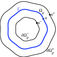
Figure 1: A cross-sectional view of the membrane $\displaystyle\Gamma$ and subdomain $\displaystyle{\Omega_{\varrho}(t)}$, having inner and outer surfaces $\displaystyle{\partial\Omega_{\varrho}^{-}(t)}$ and $\displaystyle{\partial\Omega_{\varrho}^{+}(t)}$ respectively, which illustrates the limiting process as $\displaystyle\boldsymbol{x}^{+},\boldsymbol{x}^{-}\to\boldsymbol{x}$ and $\displaystyle\varrho\to 0$.

Next, consider the divergence condition (9b) which must be satisfied identically on either side of the membrane so that

$$\displaystyle\llbracket\boldsymbol{\nabla}\boldsymbol{\cdot}\boldsymbol{u}_{1}\rrbracket=0.$$ (15)

Rewriting this condition in terms of the components of $\displaystyle\boldsymbol{u}_{1}$, we have

$$\displaystyle\bigg{\llbracket}\frac{\partial u^{r}}{\partial r}+\frac{2}{r}\,u^{r}-\frac{m(m+1)}{r}\,u^{\Psi}\bigg{\rrbracket}=\bigg{\llbracket}\frac{\partial u^{r}}{\partial r}\bigg{\rrbracket}=0,$$ (16)

where the last equality follows from (14).

The remaining jump conditions are derived from the momentum equations (9a). Letting $\displaystyle\varphi(\boldsymbol{x})$ be a smooth test function with compact support, we multiply the momentum equations by $\displaystyle\varphi(\boldsymbol{x})$ and integrate over $\displaystyle{\Omega_{\varrho}(t)}$ to obtain

$$\displaystyle\int_{\Omega_{\varrho}(t)}\left(\frac{\partial\boldsymbol{u}}{\partial t}+\boldsymbol{u}\boldsymbol{\cdot}\boldsymbol{\nabla}\boldsymbol{u}\right)\varphi(\boldsymbol{x})\;\mathrm{d}V=\int_{\Omega_{\varrho}(t)}\left(-\boldsymbol{\nabla}p+\nu\Delta\boldsymbol{u}+\boldsymbol{f}\right)\varphi(\boldsymbol{x})\;\mathrm{d}V.$$ (17)

We now examine each term in this equation in the limit as $\displaystyle\varrho\to 0$. Starting with the left-hand side, we apply the Reynolds transport theorem to extract the time derivative:

$$\displaystyle\int_{\Omega_{\varrho}(t)}\left(\frac{\partial\boldsymbol{u}}{\partial t}+\boldsymbol{u}\boldsymbol{\cdot}\boldsymbol{\nabla}\boldsymbol{u}\right)\varphi(\boldsymbol{x})\;\mathrm{d}V=\frac{\mathrm{d}}{\mathrm{d}t}\int_{\Omega_{\varrho}(t)}\boldsymbol{u}\varphi(\boldsymbol{x})\;\mathrm{d}V.$$

Because $\displaystyle\varphi(\boldsymbol{x})$ is smooth and $\displaystyle\boldsymbol{u}$ is bounded, we have that

$$\displaystyle\lim_{\varrho\to 0}\frac{\mathrm{d}}{\mathrm{d}t}\int_{\Omega_{\varrho}(t)}\boldsymbol{u}\varphi(\boldsymbol{x})\;\mathrm{d}V=0.$$ (18)

Considering next the pressure term in the right-hand side of (17), integrate by parts to obtain

$$\displaystyle\int_{\Omega_{\varrho}(t)}-\boldsymbol{\nabla}p\,\varphi(\boldsymbol{x})\;\mathrm{d}V=-\int_{{\partial\Omega_{\varrho}^{+}(t)}}p\hat{\boldsymbol{n}}\,\varphi(\boldsymbol{x})\;\mathrm{d}A+\int_{{\partial\Omega_{\varrho}^{-}(t)}}p\hat{\boldsymbol{n}}\,\varphi(\boldsymbol{x})\;\mathrm{d}A+\int_{\Omega_{\varrho}(t)}p\,\boldsymbol{\nabla}\varphi(\boldsymbol{x})\;\mathrm{d}V,$$ (19)

where $\displaystyle\hat{\boldsymbol{n}}$ is the unit outward normal vector defined by

$$\displaystyle\hat{\boldsymbol{n}}=\frac{\frac{\partial\boldsymbol{X}}{\partial\eta}\times\frac{\partial\boldsymbol{X}}{\partial\xi}}{\left\|\frac{\partial\boldsymbol{X}}{\partial\eta}\times\frac{\partial\boldsymbol{X}}{\partial\xi}\right\|}.$$ (20)

Because $\displaystyle p$ is also bounded, the last term in (19) vanishes as $\displaystyle\varrho\to 0$ and we are left with the difference between two surface integrals, which reduces to a jump in pressure; in other words,

$$\displaystyle\int_{\Omega_{\varrho}(t)}-\boldsymbol{\nabla}p\varphi(\boldsymbol{x})\;\mathrm{d}V\quad\to\quad-\int_{\Gamma}\llbracket p\rrbracket\hat{\boldsymbol{n}}\varphi(\boldsymbol{x})\;\mathrm{d}A\qquad\mbox{ as }\varrho\to 0.$$ (21)

In an analogous manner, the viscous term in (17) can be integrated by parts to yield

$$\displaystyle\int_{\Omega_{\varrho}(t)}\nu\Delta\boldsymbol{u}\varphi(\boldsymbol{x})\;\mathrm{d}V\quad\to\quad\int_{\Gamma}\nu\llbracket\hat{\boldsymbol{n}}\boldsymbol{\cdot}\boldsymbol{\nabla}\boldsymbol{u}\rrbracket\varphi(\boldsymbol{x})\;\mathrm{d}A\qquad\mbox{ as }\varrho\to 0.$$ (22)

Finally, we consider the forcing term in (17) and apply the sifting property of the Dirac delta function to obtain

$$\displaystyle\int_{\Omega_{\varrho}(t)}\boldsymbol{f}\varphi(\boldsymbol{x})\;\mathrm{d}V \displaystyle=\int_{\Omega_{\varrho}(t)}\int_{0}^{\pi}\int_{0}^{2\pi}\boldsymbol{F}\delta(\boldsymbol{x}-\boldsymbol{X})\sin\eta\;\mathrm{d}\xi\;\mathrm{d}\eta\;\varphi(\boldsymbol{x})\;\mathrm{d}V,$$

$$\displaystyle=\int_{0}^{\pi}\int_{0}^{2\pi}\boldsymbol{F}\varphi(\boldsymbol{X})\sin\eta\;\mathrm{d}\xi\;\mathrm{d}\eta.$$ (23)

The results in (18) and (21)–(23) can then be substituted into (17), after which we take the limit as $\displaystyle\varrho\to 0$ to get

$$\displaystyle 0=\int_{0}^{\pi}\int_{0}^{2\pi}\left(-\llbracket p\rrbracket\hat{\boldsymbol{n}}\left\|\frac{\partial\boldsymbol{X}}{\partial\eta}\times\frac{\partial\boldsymbol{X}}{\partial\xi}\right\|+\nu\llbracket\hat{\boldsymbol{n}}\boldsymbol{\cdot}\boldsymbol{\nabla}\boldsymbol{u}\rrbracket\left\|\frac{\partial\boldsymbol{X}}{\partial\eta}\times\frac{\partial\boldsymbol{X}}{\partial\xi}\right\|+\boldsymbol{F}\sin\eta\right)\varphi(\boldsymbol{X})\;\mathrm{d}\xi\;\mathrm{d}\eta,$$

where we have also made use of the identity

$$\displaystyle dA=\left\|\frac{\partial\boldsymbol{X}}{\partial\eta}\times\frac{\partial\boldsymbol{X}}{\partial\xi}\right\|\;\mathrm{d}\xi\;\mathrm{d}\eta.$$

Because $\displaystyle\varphi$ is arbitrary and smooth, the integrand must be identically zero, which yields

$$\displaystyle 0=-\llbracket p\rrbracket\left(\frac{\partial\boldsymbol{X}}{\partial\eta}\times\frac{\partial\boldsymbol{X}}{\partial\xi}\right)+\nu\bigg{\llbracket}\left(\frac{\partial\boldsymbol{X}}{\partial\eta}\times\frac{\partial\boldsymbol{X}}{\partial\xi}\right)\boldsymbol{\cdot}\boldsymbol{\nabla}\boldsymbol{u}\bigg{\rrbracket}+\boldsymbol{F}\sin\eta,$$ (24)

where the normal vector has been replaced using (20).

We now make use of the perturbation expansion for $\displaystyle\boldsymbol{X}$ to write the terms arising from the normal vector as

$$\displaystyle\frac{\partial\boldsymbol{X}}{\partial\eta}\times\frac{\partial\boldsymbol{X}}{\partial\xi} \displaystyle=\frac{\partial}{\partial\eta}\left(\hat{r}+\epsilon\boldsymbol{X}_{1}+O(\epsilon^{2})\right)\times\frac{\partial}{\partial\xi}\left(\hat{r}+\epsilon\boldsymbol{X}_{1}+O(\epsilon^{2})\right),$$

$$\displaystyle=\sin\eta\,\hat{r}+\epsilon\sin\eta\Big{[}(2X^{r}-m(m+1)X^{\Psi})\boldsymbol{Y}_{m,k}^{c}$$

$$\displaystyle\qquad\qquad\qquad\qquad+\,(X^{\Psi}-X^{r})\boldsymbol{\Psi}_{m,k}^{c}+X^{\Phi}\boldsymbol{\Phi}_{m,k}^{c}\Big{]}+O(\epsilon^{2}).$$

Similarly, the force density can be expanded as

$$\displaystyle\boldsymbol{F} \displaystyle=K(t)\Delta_{\xi}\left(\hat{r}+\epsilon\boldsymbol{X}_{1}+O(\epsilon^{2})\right),$$

$$\displaystyle=-2K(t)\hat{r}+\epsilon K(t)\Big{[}\left(2m(m+1)X^{\Psi}-(m^{2}+m+2)X^{r}\right)\boldsymbol{Y}_{m,k}^{c}$$

$$\displaystyle\qquad\qquad+\,\left(2X^{r}-m(m+1)X^{\Psi}\right)\boldsymbol{\Psi}_{m,k}^{c}-m(m+1)X^{\Phi}\boldsymbol{\Phi}_{m,k}^{c}\Big{]}+O(\epsilon^{2}).$$

The remaining jump conditions are obtained by substituting these last two equations along with the perturbation expansions for $\displaystyle\boldsymbol{u}$ and $\displaystyle p$ into (24). The radial component of (24) gives two jump conditions for the pressure variables

$$\displaystyle\llbracket p_{0}\rrbracket \displaystyle=-2K(t),$$ (25)

$$\displaystyle\llbracket p_{1}\rrbracket \displaystyle=-K(t)(m-1)(m+2)X^{r}Y_{m,k}^{c},$$ (26)

while the $\displaystyle\boldsymbol{\Psi}_{m,k}$ and $\displaystyle\boldsymbol{\Phi}_{m,k}$ components give jump conditions for the radial derivatives of $\displaystyle u^{\Psi}$ and $\displaystyle u^{\Phi}$

$$\displaystyle\nu\bigg{\llbracket}\frac{\partial u^{\Psi}}{\partial r}\bigg{\rrbracket} \displaystyle=K(t)(m-1)(m+2)X^{\Psi},$$ (27)

$$\displaystyle\nu\bigg{\llbracket}\frac{\partial u^{\Phi}}{\partial r}\bigg{\rrbracket} \displaystyle=K(t)(m-1)(m+2)X^{\Phi}.$$ (28)

Note that the right-hand sides of each jump condition are completely decoupled, which is the major advantage to our particular choice of VSH basis that we referred to earlier in section 2.3.

We can now summarise the system of equations that will be analysed in the remainder of this paper:

$$\displaystyle\frac{\partial u^{r}}{\partial t} \displaystyle=-\frac{\partial\hat{p}}{\partial r}+\nu\left(\Delta u^{r}-\frac{2}{r^{2}}\,u^{r}+\frac{2m(m+1)}{r^{2}}\,u^{\Psi}\right),$$ (29)

$$\displaystyle\frac{\partial u^{\Psi}}{\partial t} \displaystyle=-\frac{\hat{p}}{r}+\nu\left(\Delta u^{\Psi}+\frac{2}{r^{2}}\,u^{r}\right),$$ (30)

$$\displaystyle\frac{\partial u^{\Phi}}{\partial t} \displaystyle=\nu\Delta u^{\Phi},$$ (31)

$$\displaystyle\boldsymbol{\nabla}\cdot\boldsymbol{u}_{1} \displaystyle=\left(\frac{1}{r^{2}}\frac{\partial}{\partial r}(r^{2}u^{r})-\frac{m(m+1)}{r}\,u^{\Psi}\right)Y_{m,k}^{c}=0,$$ (32)

$$\displaystyle\frac{\partial\boldsymbol{X}_{1}}{\partial t} \displaystyle=\boldsymbol{u}_{1}|_{r=1}.$$ (33)

The scalar Laplacian operator simplifies to

$$\displaystyle\Delta=\frac{1}{r^{2}}\frac{\partial}{\partial r}\left(r^{2}\frac{\partial}{\partial r}\right)-\frac{m(m+1)}{r^{2}},$$

and the $\displaystyle O(\epsilon)$ quantities $\displaystyle\boldsymbol{X}_{1}$, $\displaystyle\boldsymbol{u}_{1}$ and $\displaystyle p_{1}$ are also subject to the jump conditions (14), (16) and (26)–(28). Note that the equation for $\displaystyle u^{\Phi}$ is totally decoupled which is another advantage of our choice of VSH basis. We also observe that the dynamics of the linearised solution depend only on the degree $\displaystyle m$ of the spherical harmonic and not on its order $\displaystyle k$; hence solution modes are characterised by a single integer $\displaystyle m$.

In the remainder of this paper, we will drop the subscript “1” that until now has distinguished the $\displaystyle O(\epsilon)$ quantities.

3 Floquet analysis for an inviscid fluid

To afford some insight into parametric instabilities occurring in a simpler version of the immersed membrane problem, we first consider an inviscid fluid for which the governing equations reduce to

$$\displaystyle\frac{\partial u^{r}}{\partial t} \displaystyle=-\frac{\partial\hat{p}}{\partial r},$$ (34a)

$$\displaystyle\frac{\partial u^{\Psi}}{\partial t} \displaystyle=-\frac{\hat{p}}{r},$$ (34b)

$$\displaystyle\frac{\partial u^{\Phi}}{\partial t} \displaystyle=0,$$ (34c)

$$\displaystyle\boldsymbol{\nabla}\boldsymbol{\cdot}\boldsymbol{u} \displaystyle=0,$$ (34d)

$$\displaystyle\frac{\mathrm{d}X^{r}}{\mathrm{d}t} \displaystyle=u^{r}(1,t),$$ (34e)

$$\displaystyle\llbracket u^{r}\rrbracket \displaystyle=0,$$ (34f)

$$\displaystyle\llbracket\hat{p}\rrbracket \displaystyle=-K(t)(m-1)(m+2)X^{r}.$$ (34g)

Notice that in the absence of viscosity, we are only permitted to impose the zero normal flow condition (34e) at the fluid-membrane interface instead of the usual no-slip condition.

We begin by solving for the pressure away from the membrane, which satisfies

$$\displaystyle\Delta\hat{p}=r^{2}\frac{\partial^{2}\hat{p}}{\partial r^{2}}+2r\frac{\partial\hat{p}}{\partial r}-m(m+1)\hat{p}=0.$$ (35)

Imposing the requirement that the pressure be bounded at $\displaystyle r=0$ and as $\displaystyle r\to\infty$ yields

$$\displaystyle\hat{p}(r,t)=\begin{cases}a(t)\,r^{m},&\mbox{if }r<1,\\ b(t)\,r^{-m-1},&\mbox{if }r>1,\end{cases}$$

where $\displaystyle a(t)$ and $\displaystyle b(t)$ are as-yet undetermined functions of time. Substituting the pressure solution into the inviscid momentum equation (34a) yields the radial fluid acceleration

$$\displaystyle\frac{\partial u^{r}}{\partial t}=\begin{cases}-ma(t)\,r^{m-1},&\mbox{if }r<1,\\ (m+1)b(t)\,r^{-m-2},&\mbox{if }r>1.\end{cases}$$

Since the fluid cannot pass through the membrane, the radial acceleration of the fluid and membrane must match and

$$\displaystyle\frac{\mathrm{d}^{2}X^{r}}{\mathrm{d}t^{2}}=\left.\frac{\partial u^{r}}{\partial t}\right|_{r=1}=-ma(t)=(m+1)b(t),$$ (36)

where the last equality follows from continuity of $\displaystyle u^{r}$ at the interface. This allows us to determine the functions

$$\displaystyle a(t)=-\frac{1}{m}\frac{\mathrm{d}^{2}X^{r}}{\mathrm{d}t^{2}}\qquad\text{and}\qquad b(t)=\frac{1}{m+1}\frac{\mathrm{d}^{2}X^{r}}{\mathrm{d}t^{2}},$$

after which the pressure jump (34g) may be expressed as

$$\displaystyle b(t)-a(t)=-K(t)(m-1)(m+2)X^{r}(t).$$ (37)

We then have the following equation for the membrane location

$$\displaystyle\frac{\mathrm{d}^{2}X^{r}}{\mathrm{d}t^{2}}+\widetilde{\omega}^{2}(1+2\tau\sin t)X^{r}=0,$$ (38)

where

$$\displaystyle\widetilde{\omega}^{2}=\frac{\kappa m(m-1)(m+1)(m+2)}{2m+1}.$$

Recalling the definition of $\displaystyle\kappa$ in (11), we may write $\displaystyle\widetilde{\omega}=\omega_{N}/\omega$ as the ratio of the natural frequency $\displaystyle\omega_{N}$ for the unforced problem to the forcing frequency $\displaystyle\omega$, where

$$\displaystyle\omega_{N}^{2}=\frac{\sigma m(m-1)(m+1)(m+2)}{\rho R^{3}(2m+1)}.$$ (39)

This natural oscillation frequency matches exactly with the classical result of Lamb (1932, Art. 253) for oscillations of a spherical liquid drop, with the only difference being that a surface tension force replaces the elastic restoring force in our IB context.

We now focus on (38) which describes a harmonic oscillator with a time-dependent frequency parameter, and hence takes the form of the well-known Mathieu equation (Nayfeh, 1993). We invoke the Floquet theory and look for a series solution of the form

$$\displaystyle X^{r}(t)=e^{\gamma t}\sum_{n=-\infty}^{\infty}X^{r}_{n}e^{\mathrm{i}nt},$$

where $\displaystyle\gamma\in\mathbb{C}$ is the Floquet exponent that determines the stability of solution as $\displaystyle t\to\infty$. Substituting this series expansion into (38) yields the following infinite system of linear algebraic equations:

$$\displaystyle-\mathrm{i}\left[\frac{(\gamma+\mathrm{i}n)^{2}}{\widetilde{\omega}^{2}}+1\right]X^{r}_{n}=\tau(X^{r}_{n-1}-X^{r}_{n+1})\qquad\text{for }n\in\mathbb{Z}.$$ (40)

Our aim is now to investigate all non-trivial solutions of this system and determine what (if any) instabilities can arise, and for what parameter values they occur. To this end, we use the standard approach and restrict ourselves to periodic solutions having $\displaystyle\mbox{Re}\{\gamma\}=0$ (i.e., neutral stability) and corresponding to two special values of the Floquet exponent: $\displaystyle\gamma=0$ (harmonic modes) and $\displaystyle\textstyle{\gamma=\frac{1}{2}\mathrm{i}}$ (subharmonic modes). It is possible to show that all other values of $\displaystyle\mbox{Im}\{\gamma\}$ lead to modes that decay in time. To ensure that the resulting solutions are real-valued functions, we impose a set of reality conditions on the Fourier series coefficients, which for the harmonic case are

$$\displaystyle X^{r}_{-n}=\overline{X}^{r}_{n},$$ (41)

whereas for the subharmonic case

$$\displaystyle X^{r}_{-n}=\overline{X}^{r}_{n-1},$$ (42)

for all $\displaystyle n\in\mathbb{Z}$. Either set of reality conditions implies that it is only necessary to consider non-negative values of $\displaystyle n$, and so the linear system (40) may be written as

$$\displaystyle A_{n}X^{r}_{n}=\tau(X^{r}_{n-1}-X^{r}_{n+1}),$$ (43)

now with $\displaystyle n=0,1,2,\dots$. For the purposes of our stability analysis, the forcing amplitude $\displaystyle\tau$ is treated as an unknown, and in practice, we approximate the infinite linear system by truncating at a finite number of modes $\displaystyle N$. The resulting equations may be written compactly in matrix form as

$$\displaystyle\mathsfbi{A}\boldsymbol{v}=\tau\mathsfbi{B}\boldsymbol{v}$$

where the unknown series coefficients are collected together in a vector

$$\displaystyle\boldsymbol{v}=\left[\begin{array}[]{c}\vdots\\ \mbox{Re}\{X^{r}_{n}\}\\ \mbox{Im}\{X^{r}_{n}\}\\ \vdots\end{array}\right],$$

and $\displaystyle\mathsfbi{A}=\mbox{diag}(\mathsfbi{A}_{0},\mathsfbi{A}_{1},\ldots,\mathsfbi{A}_{N})$ is a block diagonal matrix with $\displaystyle 2\times 2$ blocks

$$\displaystyle\mathsfbi{A}_{n}=\left[\begin{array}[]{rr}\mbox{Re}\{A_{n}\}&-\mbox{Im}\{A_{n}\}\\ \mbox{Im}\{A_{n}\}&\mbox{Re}\{A_{n}\}\\ \end{array}\right].$$

Similarly, $\displaystyle\mathsfbi{B}$ has a block tridiagonal structure of the form

$$\displaystyle\mathsfbi{B}=\left[\begin{array}[]{rrrrr}{\widehat{\mathsfbi{B}\mkern 3.0mu}{}}\mkern-3.0mu&{\widetilde{\mathsfbi{B}\mkern 3.0mu}{}}\mkern-3.0mu&&&\\ \mathsfbi{I}_{2}&\mathsfbi{0}_{2}&-\mathsfbi{I}_{2}&&\\ &\mathsfbi{I}_{2}&\mathsfbi{0}_{2}&-\mathsfbi{I}_{2}&\\ &&\ddots&\ddots&\ddots\end{array}\right],$$

where $\displaystyle\mathsfbi{0}_{2}$ and $\displaystyle\mathsfbi{I}_{2}$ denote the $\displaystyle 2\times 2$ zero and identity matrices respectively. The sub-matrices making up the first block rows of $\displaystyle A$ and $\displaystyle B$ depend on the value of $\displaystyle\gamma$, so that for the harmonic case (with $\displaystyle\gamma=0$)

$$\displaystyle\mathsfbi{A}_{0}=I,\qquad{\widehat{\mathsfbi{B}\mkern 3.0mu}\mkern-3.0mu}{}=\left[\begin{array}[]{rr}0&2\\ 0&0\end{array}\right],\qquad{\widetilde{\mathsfbi{B}\mkern 3.0mu}\mkern-3.0mu}{}=\mathsfbi{0}_{2},$$

while for the subharmonic case (with $\displaystyle\gamma=\textstyle\frac{1}{2}\mathrm{i}$)

$$\displaystyle\mathsfbi{A}_{0}=\left[\begin{array}[]{rr}\mbox{Re}\{A_{0}\}&-\mbox{Im}\{A_{0}\}\\ \mbox{Im}\{A_{0}\}&\mbox{Re}\{A_{0}\}\\ \end{array}\right],\qquad{\widehat{\mathsfbi{B}\mkern 3.0mu}\mkern-3.0mu}{}=\left[\begin{array}[]{rr}1&0\\ 0&-1\end{array}\right],\qquad{\widetilde{\mathsfbi{B}\mkern 3.0mu}\mkern-3.0mu}{}=-\mathsfbi{I}_{2}.$$

Equation (43) can be viewed as a generalised eigenvalue problem with eigenvalue $\displaystyle\tau$ and eigenvector $\displaystyle\boldsymbol{v}$. Therefore, determining the stability of the parametrically forced spherical membrane reduces to finding all values of $\displaystyle\tau$ and $\displaystyle\boldsymbol{v}$ for the two Floquet exponents $\displaystyle\gamma=0$ and $\displaystyle\textstyle{\frac{1}{2}\mathrm{i}}$ (corresponding to the harmonic and subharmonic cases respectively).

A particularly effective way of visualising these solutions is to vary one of the system parameters (either forcing frequency or elastic stiffness) and to consider the stability regions that are generated as the eigenvalues trace out curves in parameter space. This diagram is referred to as an Ince-Strutt diagram (Nayfeh, 1993), three of which are depicted in figure 3 as plots of $\displaystyle\kappa$ versus $\displaystyle\tau$ for three different spherical harmonics, $\displaystyle m=2$, 3 and 4. The stability boundaries take the form of fingers or tongues that extend downward in parameter space. There are clearly two distinct sets of alternating fingers corresponding to harmonic and subharmonic modes, which we denote using the two point types $\displaystyle+$ and $\displaystyle\bigcirc$ respectively. Parameter values lying above and inside any given finger correspond to unstable solutions, whereas all parameters lying below the fingers correspond to stable solutions. It is essential to keep in mind that only parameters lying below the horizontal line $\displaystyle{\textstyle\tau=\frac{1}{2}}$ are physically relevant, since these values of $\displaystyle\tau$ correspond to a membrane stiffness $\displaystyle K(t)$ that remains positive.

Figure 2: On the left are Ince-Strutt diagrams for the inviscid problem, showing stability contours for spherical harmonics $\displaystyle m=2$ (top), 3 (middle) and 4 (bottom). Subharmonic modes are denoted with $\displaystyle\bigcirc$ and harmonic modes with $\displaystyle+$, and only modes with $\displaystyle\textstyle\tau<\frac{1}{2}$ are physically relevant. To the right of each Ince-Strutt diagram is a picture showing spherical shells perturbed non-negative $\displaystyle k$-modes.

It is evident from these diagrams that for a given forcing amplitude $\displaystyle\tau$, an immersed spherical shell can experience parametric instability for a disjoint set of $\displaystyle\kappa$ ranges (with corresponding ranges of the physical parameters $\displaystyle\omega$, $\displaystyle\rho$, $\displaystyle R$ and $\displaystyle\sigma$ according to (11)). For example, different unstable modes (corresponding to different integer values of $\displaystyle m$) can be excited by forcing the system within a given range of $\displaystyle\omega$. Furthermore, there are an infinite number of unstable modes that can be excited since the harmonic and subharmonic fingers continue to alternate to the right forever as $\displaystyle\kappa$ increases.

These membrane instabilities exist for all values of forcing amplitude $\displaystyle 0<\textstyle\tau<\frac{1}{2}$ since each of the stability fingers extends downward and touches the $\displaystyle\kappa$-axis as $\displaystyle\tau\to 0$. The points at which the fingers touch down correspond to the natural oscillation frequencies $\displaystyle\omega_{N}$ for the unforced problem given in (39). Indeed, we see that for $\displaystyle|\tau|\ll 1$, resonances occur at forcing frequencies

$$\displaystyle\frac{\omega_{N}}{\omega}=\frac{\ell}{2},$$

for any positive integer $\displaystyle\ell$; that is, the natural frequency for a given $\displaystyle m$-mode is an integer multiple of half the parametric forcing frequency. Parametric resonance is characterised by the subharmonic modes (odd $\displaystyle\ell$) where the response frequency is half the forcing frequency.

4 Floquet analysis for a viscous fluid

Guided by the analysis from the previous section, we next apply Floquet theory to the original governing equations with viscosity by looking for series solutions of the form

$$\displaystyle\boldsymbol{u}(r,\theta,\phi,t) \displaystyle=e^{\gamma t}\sum_{n=-\infty}^{\infty}e^{\mathrm{i}nt}\left(u^{r}_{n}(r)\boldsymbol{Y}_{m,k}^{c}+u^{\Psi}_{n}(r)\boldsymbol{\Psi}_{m,k}^{c}+u^{\Phi}_{n}(r)\boldsymbol{\Phi}_{m,k}^{c}\right),$$

$$\displaystyle\boldsymbol{X}(\xi,\eta,t) \displaystyle=e^{\gamma t}\sum_{n=-\infty}^{\infty}e^{\mathrm{i}nt}\left(X^{r}_{n}\boldsymbol{Y}_{m,k}^{c}+X^{\Psi}_{n}\boldsymbol{\Psi}_{m,k}^{c}+X^{\Phi}_{n}\boldsymbol{\Phi}_{m,k}^{c}\right),$$

$$\displaystyle p(r,\theta,\phi,t) \displaystyle=e^{\gamma t}\sum_{n=-\infty}^{\infty}e^{\mathrm{i}nt}p_{n}(r)Y_{m,k}^{c}.$$

The pressure coefficients $\displaystyle p_{n}(r)$ satisfy the same ODE (35) and boundedness conditions as in the inviscid case, and so the solution has the same form

$$\displaystyle p_{n}(r)=\begin{cases}a_{n}r^{m},&\mbox{if }r<1,\\[2.0pt] b_{n}r^{-m-1},&\mbox{if }r>1,\\ \end{cases}$$

with the only difference being that $\displaystyle a_{n}$ and $\displaystyle b_{n}$ are constants. Next, combining the radial momentum equation (29) with the divergence-free condition (32) yields the PDE

$$\displaystyle\frac{\partial u^{r}}{\partial t}=-\frac{\partial\hat{p}}{\partial r}+\nu\left(\Delta u^{r}-2\frac{u^{r}}{r^{2}}+\frac{2}{r}\left(\frac{1}{r^{2}}\frac{\partial}{\partial r}(r^{2}u^{r})\right)\right).$$

After substituting the series form for $\displaystyle u^{r}$ we obtain

$$\displaystyle r^{2}{u^{r}_{n}}^{\prime\prime}+4r{u^{r}_{n}}^{\prime}+\left(2-m(m+1)-\beta_{n}^{2}r^{2}\right)u^{r}_{n}-\frac{r^{2}}{\nu}\,p_{n}^{\prime}=0,$$

where primes denote derivatives with respect to $\displaystyle r$ and

$$\displaystyle\beta_{n}=\sqrt{\frac{\gamma+\mathrm{i}n}{\nu}}\quad\mbox{ with }\quad\mbox{Re}\{\beta_{n}\}>0,$$

We first consider the situation where the quantity $\displaystyle\beta_{n}\neq 0$, in which case the radial velocity component can be expressed as

$$\displaystyle u^{r}_{n}(r)=\int_{0}^{\infty}\frac{z^{2}}{\nu}\,G(r,z)p_{n}^{\prime}(z)\;\mathrm{d}z,$$ (44)

where $\displaystyle G(r,z)$ is the Green’s function satisfying

$$\displaystyle r^{2}\frac{\partial^{2}G}{\partial r^{2}}+4r\frac{\partial G}{\partial r}+(2-m(m+1)-\beta_{n}^{2}r^{2})G=\delta(r-z),$$

along with the two jump conditions

$$\displaystyle\left.G\right|_{r=z^{-}}^{r=z^{+}}=0\qquad\text{and}\qquad\left.r^{2}\frac{\partial G}{\partial r}\right|_{r=z^{-}}^{r=z^{+}}=1.$$

The Green’s function can be obtained explicitly as

$$\displaystyle G(r,z)=\begin{cases}\displaystyle z\beta_{n}h_{m}(\mathrm{i}\beta_{n}z)\,\frac{j_{m}(\mathrm{i}\beta_{n}r)}{r},&\quad\mbox{ if }r<z,\\[8.5359pt] \displaystyle z\beta_{n}j_{m}(\mathrm{i}\beta_{n}z)\,\frac{h_{m}(\mathrm{i}\beta_{n}r)}{r},&\quad\mbox{ if }r>z,\end{cases}$$

where $\displaystyle j_{m}$ and $\displaystyle h_{m}$ denote the $\displaystyle m$th-order spherical Bessel and Hankel functions of the first kind (respectively). The expression in (44) can be integrated explicitly to obtain the radial velocity as

$$\displaystyle u^{r}_{n}(r)=\left\{\begin{array}[]{lll}&\displaystyle-\frac{\mathrm{i}j_{m}(\mathrm{i}\beta_{n}r)}{\nu r}\Big{(}ma_{n}h_{m+1}(\mathrm{i}\beta_{n})-(m+1)b_{n}h_{m-1}(\mathrm{i}\beta_{n})\Big{)}\\[5.69046pt] &\displaystyle\qquad\qquad-\frac{m}{\nu\beta_{n}^{2}}a_{n}r^{m-1},&\mbox{ if }r<1,\\[8.5359pt] &\displaystyle-\frac{\mathrm{i}h_{m}(\mathrm{i}\beta_{n}r)}{\nu r}\Big{(}ma_{n}j_{m+1}(\mathrm{i}\beta_{n})-(m+1)b_{n}j_{m-1}(\mathrm{i}\beta_{n})\Big{)}\\[5.69046pt] &\qquad\qquad+\frac{m+1}{\nu\beta_{n}^{2}}b_{n}r^{-m-2},&\mbox{ if }r>1.\end{array}\right.$$

It is then straightforward to show that radial velocity coefficients are continuous across the membrane and satisfy

$$\displaystyle u_{n}^{r}(1^{+})=u_{n}^{r}(1^{-})=-\frac{\mathrm{i}m}{\nu}\,a_{n}h_{m}(\mathrm{i}\beta_{n})j_{m+1}(\mathrm{i}\beta_{n})+\frac{\mathrm{i}(m+1)}{\nu}\,b_{n}j_{m}(\mathrm{i}\beta_{n})h_{m-1}(\mathrm{i}\beta_{n}).$$

The coefficient $\displaystyle u^{\Psi}_{n}$ can be obtained by solving the incompressibility condition

$$\displaystyle\left(\frac{1}{r^{2}}\frac{\mathrm{d}}{\mathrm{d}r}\left(r^{2}u^{r}_{n}\right)-\frac{m(m+1)}{r}u^{\Psi}_{n}\right)Y_{m,k}^{c}=0,$$

so that

$$\displaystyle u^{\Psi}_{n}(r) \displaystyle=\frac{1}{rm(m+1)}\frac{\mathrm{d}}{\mathrm{d}r}\left(r^{2}u^{r}_{n}\right),$$

$$\displaystyle=\left\{\begin{array}[]{ll}&-\frac{\mathrm{i}}{\nu}\left(\frac{j_{m}(\mathrm{i}\beta_{n}r)}{r}+\mathrm{i}\beta_{n}j_{m}^{\prime}(\mathrm{i}\beta_{n}r)\right)\left(a_{n}\frac{h_{m+1}(\mathrm{i}\beta_{n})}{m+1}-b_{n}\frac{h_{m-1}(\mathrm{i}\beta_{n})}{m}\right)\\ &\qquad\qquad-\frac{1}{\nu\beta_{n}^{2}}\,a_{n}r^{m-1},\qquad\qquad\qquad\qquad\qquad\qquad\qquad\quad\;\;\;\mbox{ if }r<1,\\[8.5359pt] &-\frac{\mathrm{i}}{\nu}\left(\frac{h_{m}(\mathrm{i}\beta_{n}r)}{r}+\mathrm{i}\beta_{n}h_{m}^{\prime}(\mathrm{i}\beta_{n}r)\right)\left(a_{n}\frac{j_{m+1}(\mathrm{i}\beta_{n})}{m+1}-b_{n}\frac{j_{m-1}(\mathrm{i}\beta_{n})}{m}\right)\\ &\qquad\qquad-\frac{1}{\nu\beta_{n}^{2}}\,b_{n}r^{-m-2},\qquad\qquad\qquad\qquad\qquad\qquad\qquad\quad\;\;\mbox{ if }r>1.\end{array}\right.$$

The analogous equation for the third velocity coefficient $\displaystyle u^{\Phi}_{n}(r)$ is

$$\displaystyle r^{2}{u^{\Phi}_{n}}^{\prime\prime}+2r{u^{\Phi}_{n}}^{\prime}-(\beta_{n}^{2}r^{2}+m(m+1)){u^{\Phi}_{n}}=0,$$

which can be solved to obtain

$$\displaystyle u^{\Phi}_{n}(r)=\begin{cases}c_{n}j_{m}(\mathrm{i}\beta_{n}r),&\mbox{if }r<1,\\[5.69046pt] c_{n}\,\frac{j_{m}(\mathrm{i}\beta_{n})}{h_{m}(\mathrm{i}\beta_{n})}\,h_{m}(\mathrm{i}\beta_{n}r),&\mbox{if }r>1,\end{cases}$$

where $\displaystyle c_{n}$ are arbitrary constants.

The next major step is to determine values of the constants $\displaystyle a_{n}$, $\displaystyle b_{n}$ and $\displaystyle c_{n}$ by imposing the interface conditions (33). By orthogonality, the radial coefficients for the membrane position satisfy

$$\displaystyle(\gamma+\mathrm{i}n)X^{r}_{n} \displaystyle=u^{r}_{n}(1),$$

$$\displaystyle=-\frac{\mathrm{i}m}{\nu}\,a_{n}h_{m}(\mathrm{i}\beta_{n})j_{m+1}(\mathrm{i}\beta_{n})+\frac{\mathrm{i}(m+1)}{\nu}\,b_{n}j_{m}(\mathrm{i}\beta_{n})h_{m-1}(\mathrm{i}\beta_{n}),$$

with similar expressions holding for the other two sets of coefficients

$$\displaystyle(\gamma+\mathrm{i}n)X^{\Psi}_{n} \displaystyle=-\frac{\mathrm{i}}{(m+1)\nu}\,a_{n}\Big{(}h_{m}(\mathrm{i}\beta_{n})+\mathrm{i}\beta_{n}h_{m}^{\prime}(\mathrm{i}\beta_{n})\Big{)}j_{m+1}(\mathrm{i}\beta_{n})$$

$$\displaystyle\qquad+\frac{\mathrm{i}}{m\nu}\,b_{n}\Big{(}j_{m}(\mathrm{i}\beta_{n})+\mathrm{i}\beta_{n}h_{m}^{\prime}(\mathrm{i}\beta_{n})\Big{)}h_{m-1}(\mathrm{i}\beta_{n}),$$

$$\displaystyle(\gamma+\mathrm{i}n)X^{\Phi}_{n} \displaystyle=c_{n}j_{m}(\mathrm{i}\beta_{n}).$$

These three equations may then be solved to obtain

$$\displaystyle a_{n} \displaystyle=-\frac{\mathrm{i}\nu^{2}\beta_{n}^{3}}{m}\,\frac{j_{m}(\mathrm{i}\beta_{n})+\mathrm{i}\beta_{n}j_{m}^{\prime}(\mathrm{i}\beta_{n})}{j_{m+1}(\mathrm{i}\beta_{n})}\,X^{r}_{n}+\mathrm{i}\nu^{2}\beta_{n}^{3}(m+1)\,\frac{j_{m}(\mathrm{i}\beta_{n})}{j_{m+1}(\mathrm{i}\beta_{n})}\,X^{\Psi}_{n},$$ (45a)

$$\displaystyle b_{n} \displaystyle=-\frac{\mathrm{i}\nu^{2}\beta_{n}^{3}}{m+1}\,\frac{h_{m}(\mathrm{i}\beta_{n})+\mathrm{i}\beta_{n}\,h_{m}^{\prime}(\mathrm{i}\beta_{n})}{h_{m-1}(\mathrm{i}\beta_{n})}\,X^{r}_{n}+\mathrm{i}\nu^{2}\beta_{n}^{3}m\,\frac{h_{m}(\mathrm{i}\beta_{n})}{h_{m-1}(\mathrm{i}\beta_{n})}\,X^{\Psi}_{n},$$ (45b)

$$\displaystyle c_{n} \displaystyle=\frac{\nu\beta_{n}^{2}}{j_{m}(\mathrm{i}\beta_{n})}\,X^{\Phi}_{n}.$$ (45c)

We are now prepared to impose the jump conditions (27) and (28), which yield

$$\displaystyle\nu\left(-\frac{1}{m+1}a_{n}-\frac{1}{m}b_{n}\right) \displaystyle=\kappa(m-1)(m+2)\left(X^{\Psi}_{n}-\mathrm{i}\tau X^{\Psi}_{n-1}+\mathrm{i}\tau X^{\Psi}_{n+1}\right),$$

$$\displaystyle\nu\left(\mathrm{i}\beta_{n}\frac{j_{m}(\mathrm{i}\beta_{n})}{h_{m}(\mathrm{i}\beta_{n})}h_{m}^{\prime}(\mathrm{i}\beta_{n})-\mathrm{i}\beta_{n}j_{m}^{\prime}(\mathrm{i}\beta_{n})\right)c_{n} \displaystyle=\kappa(m-1)(m+2)\left(X^{\Phi}_{n}-\mathrm{i}\tau X^{\Phi}_{n-1}+\mathrm{i}\tau X^{\Phi}_{n+1}\right).$$

After replacing $\displaystyle a_{n}$, $\displaystyle b_{n}$ and $\displaystyle c_{n}$ in these last two expressions with (45), we then obtain the following two linear systems of equations relating the coefficients $\displaystyle X^{r}_{n}$, $\displaystyle X^{\Psi}_{n}$ and $\displaystyle X^{\Phi}_{n}$:

$$\frac{\beta_{n}^{3}}{(m-1)(m+2)}\frac{\nu^{2}}{\kappa}\left(\frac{h_{m}(\mathrm{i}\beta_{n})}{(m+1)h_{m-1}(\mathrm{i}\beta_{n})}-\frac{j_{m}(\mathrm{i}\beta_{n})}{mj_{m+1}(\mathrm{i}\beta_{n})}\right)X^{r}_{n}\\ +\left[\frac{\beta_{n}^{3}}{(m-1)(m+2)}\frac{\nu^{2}}{\kappa}\left(\frac{h_{m}(\mathrm{i}\beta_{n})}{h_{m-1}(\mathrm{i}\beta_{n})}+\frac{j_{m}(\mathrm{i}\beta_{n})}{j_{m+1}(\mathrm{i}\beta_{n})}\right)-\mathrm{i}\right]X^{\Psi}_{n}\\ =\tau\left(X^{\Psi}_{n-1}-X^{\Psi}_{n+1}\right),$$ (46)

$$\displaystyle\left[\frac{\mathrm{i}\beta_{n}}{(m-1)(m+2)j_{m}(\mathrm{i}\beta_{n})h_{m}(\mathrm{i}\beta_{n})}\frac{\nu^{2}}{\kappa}-\mathrm{i}\right]X^{\Phi}_{n}=\tau\left(X^{\Phi}_{n-1}-X^{\Phi}_{n+1}\right).$$ (47)

In a similar manner, the final jump condition for the pressure (26) yields

$$\left[-\frac{\mathrm{i}\beta_{n}^{4}}{(2m+1)(m-1)(m+2)}\frac{\nu^{2}}{\kappa}\left(2-\frac{m}{m+1}\frac{h_{m+1}(\mathrm{i}\beta_{n})}{h_{m-1}(\mathrm{i}\beta_{n})}-\frac{m+1}{m}\frac{j_{m-1}(\mathrm{i}\beta_{n})}{j_{m+1}(\mathrm{i}\beta_{n})}\right)-\mathrm{i}\right]X^{r}_{n}\\ -\frac{\mathrm{i}\beta_{n}^{4}}{(2m+1)(m-1)(m+2)}\frac{\nu^{2}}{\kappa}\left(1-m\frac{h_{m+1}(\mathrm{i}\beta_{n})}{h_{m-1}(\mathrm{i}\beta_{n})}+(m+1)\frac{j_{m-1}(\mathrm{i}\beta_{n})}{j_{m+1}(\mathrm{i}\beta_{n})}\right)X^{\Psi}_{n}\\ =\tau\left(X^{r}_{n-1}-X^{r}_{n+1}\right).$$ (51)

When taken together, equations (46)–(51) represent a solvable system for $\displaystyle X^{r}_{n}$, $\displaystyle X^{\Psi}_{n}$ and $\displaystyle X^{\Phi}_{n}$ in the case when $\displaystyle\beta_{n}\neq 0$.

We now consider the special case $\displaystyle\beta_{n}=0$, which occurs only when $\displaystyle n=0$ and $\displaystyle\gamma=0$ (i.e., for harmonic modes) and the equation for radial velocity reduces to

$$\displaystyle r^{2}{u^{r}_{0}}^{\prime\prime}+4r{u^{r}_{0}}^{\prime}+\left(2-m(m+1)\right)u^{r}_{0}-r^{2}\frac{p_{0}^{\prime}}{\nu}=0.$$

The corresponding Green’s function is

$$\displaystyle G(r,z)=-\frac{1}{2m+1}\begin{cases}\frac{r^{m-1}}{z^{m}},&\mbox{ if }r<z,\\[8.0pt] \frac{z^{m+1}}{r^{m+2}},&\mbox{ if }r>z,\end{cases}$$

from which we obtain

$$\displaystyle u^{r}_{0}(r)=\begin{cases}a_{0}\frac{m}{\nu(2m+3)}r^{m+1}-\frac{1}{\nu(2m+1)}\left(a_{0}\frac{m}{2}-b_{0}\frac{m+1}{2m-1}\right)r^{m-1},&\mbox{ if }r<1,\\[8.0pt] b_{0}\frac{m+1}{\nu(2m-1)}r^{-m}-\frac{1}{\nu(2m+1)}\left(a_{0}\frac{m}{2m+3}+b_{0}\frac{m+1}{2}\right)r^{-m-2},&\mbox{ if }r>1.\end{cases}$$ (52)

Using the incompressibility condition as before, we find that

$$\displaystyle u^{\Psi}_{0}(r)=\begin{cases}a_{0}\frac{m+3}{\nu(2m+3)(m+1)}\,r^{m+1}\\ \qquad\qquad-\,\frac{1}{\nu m(2m+1)}\,\left(a_{0}\frac{m}{2}-b_{0}\frac{m+1}{2m-1}\right)r^{m-1},&\mbox{ if }r<1,\\[8.0pt] -b_{0}\frac{m-1}{\nu m(2m-1)}\,r^{-m}\\ \qquad\qquad+\,\frac{1}{\nu(m+1)(2m+1)}\,\left(a_{0}\frac{m}{2m+3}+b_{0}\frac{m+1}{2}\right)r^{-m-2},&\mbox{ if }r>1,\end{cases}$$ (53)

and remaining velocity coefficients are given very simply by

$$\displaystyle u^{\Phi}_{0}(r)=\begin{cases}c_{0}r^{m},&\mbox{if }r<1,\\[2.0pt] c_{0}r^{-m-1},&\mbox{if }r>1.\\ \end{cases}$$ (54)

If we then substitute (52)–(54) into the membrane evolution equation (33), we obtain the following system of three linear equations

$$\displaystyle-\frac{m}{\nu(2m+3)(2m+1)}\,a_{0}+\frac{m+1}{\nu(2m-1)(2m+1)}\,b_{0} \displaystyle=0,$$

$$\displaystyle\frac{m}{\nu(m+1)(2m+3)(2m+1)}\,a_{0}+\frac{m+1}{\nu m(2m-1)(2m+1)}\,b_{0} \displaystyle=0,$$

$$\displaystyle c_{0} \displaystyle=0.$$

It is easy to show that this linear system is invertible as long as $\displaystyle m$ is a positive integer, and since the equations are homogeneous the unique solution is $\displaystyle a_{0}=b_{0}=c_{0}=0$. Therefore, in the special case $\displaystyle\beta_{n}=0$, the jump conditions (46)–(51) reduce to

$$\displaystyle X^{\Psi}_{n}-\mathrm{i}\tau X^{\Psi}_{n-1}+\mathrm{i}\tau X^{\Psi}_{n+1} \displaystyle=0,$$ (55)

$$\displaystyle X^{r}_{n}-\mathrm{i}\tau X^{\Phi}_{n-1}+\mathrm{i}\tau X^{\Phi}_{n+1} \displaystyle=0,$$ (56)

$$\displaystyle X^{r}_{n}-\mathrm{i}\tau X^{r}_{n-1}+\mathrm{i}\tau X^{r}_{n+1} \displaystyle=0.$$ (57)

To investigate the stability of a parametrically-forced elastic shell, we now need only consider the $\displaystyle\boldsymbol{Y}_{m,k}$ and $\displaystyle\boldsymbol{\Psi}_{m,k}$ solution components. This is because the $\displaystyle\boldsymbol{\Phi}_{m,k}$ component is completely decoupled in the momentum equations and neither is it driven by a pressure gradient, so that it evolves independently (this is of course closely related to the fact that the equations (47) for $\displaystyle X^{\Phi}_{n}$ are decoupled from the other equations). In particular, if the $\displaystyle\boldsymbol{\Phi}_{m,k}$ component of the initial membrane position is zero, then it will remain zero for all time. As a result, it is only necessary to consider equations (46), (51), (55) and (57), which can be written as

$$\displaystyle A_{n}X^{r}_{n}+B_{n}X^{\Psi}_{n} \displaystyle=\tau(X^{r}_{n-1}-X^{r}_{n+1}),$$ (58)

$$\displaystyle C_{n}X^{r}_{n}+D_{n}X^{\Psi}_{n} \displaystyle=\tau(X^{\Psi}_{n-1}-X^{\Psi}_{n+1}),$$ (59)

for suitably defined constants $\displaystyle A_{n}$, $\displaystyle B_{n}$, $\displaystyle C_{n}$ and $\displaystyle D_{n}$. We again impose reality conditions for either harmonic solutions ($\displaystyle\gamma=0$)

$$\displaystyle X^{r}_{-n} \displaystyle=\overline{X}^{r}_{n},$$ (60a)

$$\displaystyle X^{\Psi}_{-n} \displaystyle=\overline{X}^{\Psi}_{n},$$ (60b)

or subharmonic solutions ($\displaystyle\gamma=\textstyle\frac{1}{2}\mathrm{i}$)

$$\displaystyle X^{r}_{-n} \displaystyle=\overline{X}^{r}_{n-1},$$ (61a)

$$\displaystyle X^{\Psi}_{-n} \displaystyle=\overline{X}^{\Psi}_{n-1}.$$ (61b)

Again, we only need to consider non-negative integer values of $\displaystyle n=0,1,\dots,N$, so that equations (58)–(59) take the form of a generalised eigenvalue problem $\displaystyle\mathsfbi{A}\boldsymbol{v}=\tau\mathsfbi{B}\boldsymbol{v}$, where the solution vector

$$\displaystyle\boldsymbol{v}=\left[\begin{array}[]{c}\vdots\\ \mbox{Re}\{X^{r}_{n}\}\\[2.0pt] \mbox{Im}\{X^{r}_{n}\}\\[2.0pt] \mbox{Re}\{X^{\Psi}_{n}\}\\[2.0pt] \mbox{Im}\{X^{\Psi}_{n}\}\\ \vdots\end{array}\right].$$

is of length $\displaystyle 4(N+1)$. The matrix $\displaystyle\mathsfbi{A}=\mbox{diag}(\mathsfbi{A_{0}},\mathsfbi{A_{1}},\ldots,\mathsfbi{A_{N}})$ is block diagonal consisting of $\displaystyle 4\times 4$ blocks

$$\displaystyle\mathsfbi{A}_{n}=\left[\begin{array}[]{rrrr}\mbox{Re}\{A_{n}\}&-\mbox{Im}\{A_{n}\}&\mbox{Re}\{B_{n}\}&-\mbox{Im}\{A_{n}\}\\[2.0pt] \mbox{Im}\{A_{n}\}&\mbox{Re}\{A_{n}\}&\mbox{Im}\{B_{n}\}&\mbox{Re}\{B_{n}\}\\[2.0pt] \mbox{Re}\{C_{n}\}&-\mbox{Im}\{C_{n}\}&\mbox{Re}\{D_{n}\}&-\mbox{Im}\{D_{n}\}\\[2.0pt] \mbox{Im}\{C_{n}\}&\mbox{Re}\{C_{n}\}&\mbox{Im}\{D_{n}\}&\mbox{Re}\{D_{n}\}\\ \end{array}\right],$$

and $\displaystyle\mathsfbi{B}$ is a block tridiagonal matrix of the form

$$\displaystyle\mathsfbi{B}=\left[\begin{array}[]{rrrrr}{\widehat{\mathsfbi{B}\mkern 3.0mu}{}}\mkern-3.0mu&{\widetilde{\mathsfbi{B}\mkern 3.0mu}{}}\mkern-3.0mu&&&\\ \mathsfbi{I}_{4}&\mathsfbi{0}_{4}&-\mathsfbi{I}_{4}&&\\ &\mathsfbi{I}_{4}&\mathsfbi{0}_{4}&-\mathsfbi{I}_{4}&\\ &&\ddots&\ddots&\ddots\end{array}\right],$$

where in the harmonic case

$$\displaystyle{\widehat{\mathsfbi{B}\mkern 3.0mu}\mkern-3.0mu}{}=\left[\begin{array}[]{cccc}0&2&0&0\\ 0&0&0&0\\ 0&0&0&2\\ 0&0&0&0\end{array}\right]\qquad\text{and}\qquad{\widetilde{\mathsfbi{B}\mkern 3.0mu}\mkern-3.0mu}{}=\mathsfbi{0}_{4},$$

whereas in the subharmonic case

$$\displaystyle{\widehat{\mathsfbi{B}\mkern 3.0mu}\mkern-3.0mu}{}=\left[\begin{array}[]{rrrr}1&0&0&0\\ 0&-1&0&0\\ 0&0&1&0\\ 0&0&0&-1\\ \end{array}\right]\qquad\text{and}\qquad{\widetilde{\mathsfbi{B}\mkern 3.0mu}\mkern-3.0mu}{}=-\mathsfbi{I}_{4}.$$

To illustrate the stability of the viscous problem, we solve the eigenvalue equations for two values of the dimensionless viscosity, $\displaystyle\nu=10^{-3}$ and $\displaystyle 6\times 10^{-3}$, and for spherical harmonics numbered $\displaystyle m=2,3,4$. In the numerical calculations, we use a truncation size of $\displaystyle N=80$ so that all trailing coefficients of $\displaystyle\{X_{n}^{r},X_{n}^{\Psi}\}$ for $\displaystyle N>80$ are no larger than $\displaystyle 10^{-9}$ and so can be easily neglected. The corresponding Ince-Strutt diagrams are shown in figure 3 where again we observe a clearly defined sequence of alternating harmonic and subharmonic fingers of instability in parameter space. These results reinforce one of the defining characteristics of parametric resonance, namely that such systems can experience instabilities leading to unbounded growth even in the presence of damping.

There are few key comparisons that can be drawn with the inviscid results from section 3. First of all, the stability fingers do not touch the $\displaystyle\kappa$-axis as they did in the inviscid case, but instead are shifted vertically upwards. As a result, there is a minimum forcing amplitude required to initiate resonance for any given value of $\displaystyle\kappa$. For the smaller value of viscosity $\displaystyle\nu=10^{-3}$ the fingers appear most similar to the inviscid case, while for larger $\displaystyle\nu$ the fingers deform upwards away from the $\displaystyle\kappa$-axis and shift outward to the right. Indeed, for large enough values of either viscosity or spherical harmonic $\displaystyle m$ the fingers can lift entirely above the line $\displaystyle\tau=\textstyle\frac{1}{2}$ so that resonant behaviour is no longer possible. This should be contrasted with the inviscid case where resonances exist for any value of $\displaystyle m$.

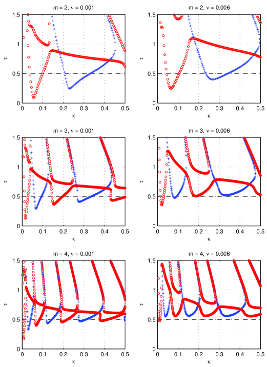
Figure 3: Ince-Strutt diagrams for the original viscous problem with dimensionless viscosities $\displaystyle\nu=10^{-3}$ (left) and $\displaystyle\nu=6\times 10^{-3}$ (right). Stability contours are shown for spherical harmonics $\displaystyle m=2$ (top), 3 (middle) and 4 (bottom). Subharmonic solutions are denoted with $\displaystyle\bigcirc$ and harmonic solutions with $\displaystyle+$.

The second distinction from the inviscid results is that within the non-physical region $\displaystyle\textstyle\tau>\frac{1}{2}$, an additional subharmonic solution appears as a curve of circular points that cuts across the finger-shaped contours. These unstable modes occur due to the periodic modulation in the tangential stress across the membrane (28) and thus are not observed in the inviscid case. However, all of these modes are restricted to the non-physical region $\displaystyle\textstyle\tau>\frac{1}{2}$ and so they can be considered as spurious and safely ignored.

5 Numerical simulations

Our next aim is to verify the existence of parametric instabilities for an internally forced spherical membrane using numerical simulations of the full governing equations (9). We use a parallel implementation of the immersed boundary algorithm of Wiens (2014) and Wiens & Stockie (2014) that utilises a pseudo-compressible Navier-Stokes solver having particular advantages in terms of parallel speed-up on distributed clusters. The algorithm exploits a rectangular fluid domain with periodic boundary conditions, but we found that a cubic computational domain with side length $\displaystyle 6R$ is sufficiently large to avoid significant interference from the adjacent periodic shells. The elastic shell is discretised using a triangulated mesh generated with the Matlab code distmesh (Persson & Strang, 2004), wherein each vertex is an IB node and each edge in the triangulation is a force-generating spring link that joins adjacent nodes. The elastic force generated by the deformed membrane is then simply the sum of all spring forces arising from this network of stretched springs. The membrane is given an initial configuration

$$\displaystyle\boldsymbol{X}(\xi,\eta,0)=R\big{(}1+\epsilon Y_{m,k}^{c}(\xi,\eta)\big{)}\,\hat{r},$$

corresponding to a chosen scalar spherical harmonic of degree $\displaystyle m$ and order $\displaystyle k$ with perturbation amplitude

$$\displaystyle\epsilon=\frac{0.05}{\displaystyle\max_{\xi,\eta}\left|Y_{m,k}^{c}(\xi,\eta)\right|}\,.$$

We then performed numerical simulations for four different sets of parameters listed in table 1, which we refer to as cases 1–4. This table lists the physical parameters used in the simulations ($\displaystyle\rho$, $\displaystyle\mu$, $\displaystyle R$, $\displaystyle\omega$, $\displaystyle\sigma$) as well as the corresponding dimensionless parameters appearing in our analytical results ($\displaystyle\nu$, $\displaystyle\kappa$). The corresponding stability contours for each case 1–4 are shown in figure 4, this time in terms of plots of $\displaystyle\tau$ versus $\displaystyle m$ holding the values of $\displaystyle\nu$ and $\displaystyle\kappa$ fixed. This alternate view of the stability regions allows us to identify the unstable modes that correspond to physical oscillations, since only modes with integer values of $\displaystyle m$ are actually observable.

Case		$\displaystyle\nu$	$\displaystyle\kappa$		$\displaystyle\rho$ ($\displaystyle\mbox{g/cm}^{3}$)	$\displaystyle R$ (cm)	$\displaystyle\omega$ ($\displaystyle 1/\mbox{s}$)	$\displaystyle\mu$ (g/cm s)	$\displaystyle\sigma$ ($\displaystyle\mbox{g/s}^{2}$)
1		0.006	0.02		1	1	1	0.006	0.02
2		0.002	0.06		1	0.5	20	0.01	3
3		0.001	0.0075		1	0.5	20	0.005	0.375
4		0.004	0.25		1	10	0.05	0.02	0.625

Table 1: Dimensionless and physical parameters for the four test cases.

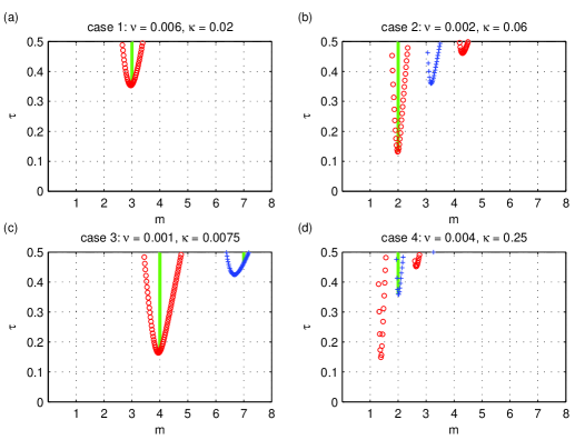
Figure 4: Ince-Strutt plots showing stability contours for each test case 1–4. Parameters that give rise to observable instabilities (i.e., corresponding to integer values of $\displaystyle m$) are highlighted by a vertical green line.

Numerical simulations are performed by initialising the membrane with various ($\displaystyle m$,$\displaystyle k$)-modes lying inside and outside the highlighted unstable fingers so that direct comparisons can be drawn with our analytical results. Figure 5 depicts several snapshots of the numerical solution for case 1, where the membrane was perturbed by a $\displaystyle(3,0)$-mode. The parametric forcing amplitude was set to $\displaystyle\tau=0.45$ which is well within the stability finger in figure 4a. Over time, the small initial perturbation grows and oscillates with a frequency equal to one-half that of the forcing frequency, as expected from the linear analysis. To help visualise the growth of this mode over time, we compute the projection

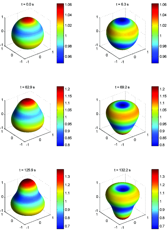
Figure 5: Several snapshots from the case 1 simulation where the membrane was initialised with a $\displaystyle(3,0)$-mode and the forcing amplitude is set to $\displaystyle\tau=0.45$.

$$\displaystyle\widehat{X}^{r}(t)=\int_{0}^{\pi}\int_{0}^{2\pi}\boldsymbol{X}\boldsymbol{\cdot}\boldsymbol{Y}_{m,k}^{c}\sin\eta\;\mathrm{d}\xi\;\mathrm{d}\eta$$

at each time. This integral is computed by first interpolating the IB mesh values of $\displaystyle\boldsymbol{X}$ onto a regular $\displaystyle(\xi,\eta)$ grid and then approximating the integral numerically using a Fast Fourier Transform in $\displaystyle\xi$ and Gauss-Legendre quadrature in $\displaystyle\eta$. Figure 6 depicts the evolution of $\displaystyle\widehat{X}^{r}(t)$ for the $\displaystyle(3,0)$-mode, from which it is easy to see the expected period-doubling response to a waveform with period $\displaystyle 4\pi$. To illustrate that the membrane instability depends sensitively on the choice of mode, figure 6 also shows simulations that were perturbed with $\displaystyle(2,0)$ and $\displaystyle(4,0)$-modes; neither of these two other modes exhibits any evidence of instability, which is also predicted by the stability plots in figure 4a.

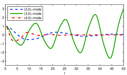
Figure 6: Radial amplitude projection $\displaystyle\widehat{X}^{r}$ for case 1, with the spherical shell perturbed by three different $\displaystyle(m,k)$-modes. The results are all rescaled to start at $\displaystyle\widehat{X}^{r}=1$.

One conclusion from our analysis is that for each $\displaystyle m$, the stability of the linearised dynamics does not depend on the order $\displaystyle k$ of the spherical harmonic. This result is investigated in figure 7, where we display the projected radial amplitude $\displaystyle\widehat{X}^{r}$ for two simulations using the case 1 parameters and two initial membrane shapes corresponding to modes $\displaystyle(3,0)$ and $\displaystyle(3,1)$. The analytical solution is provided for comparison, and we observe that the behaviour of all three solution curves is nearly indistinguishable at early times. However, as time goes on the perturbations grow and non-linear affects come into play in the simulations, so that the growth rates eventually deviate from the linear analysis.

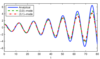
Figure 7: Radial amplitude projection $\displaystyle\widehat{X}^{r}$ in case 1, showing a spherical shell perturbed by a $\displaystyle(3,0)$-mode (dashed) and a $\displaystyle(3,1)$-mode (dash-dot). The exact result from the linear analysis is shown as a solid line. All curves are rescaled to start at $\displaystyle\widehat{X}^{r}=1$.

As another illustration of the dependence of stability on system parameters, we perform a series of simulations to investigate the “sharpness” of the stability fingers. Using parameters from case 2, we fix $\displaystyle\tau=0.25$ and then investigate the behaviour of the numerical solution as $\displaystyle\kappa$ is varied. Based on figure 4b, we expect case 2 to be unstable if the membrane configuration is an $\displaystyle m=2$ mode, but if parameters are changed sufficiently then the stability fingers can shift enough that the 2-mode stabilises. Figure 8a shows the Ince-Strutt diagram as a plot of $\displaystyle\tau$ versus $\displaystyle\kappa$ for $\displaystyle\nu=0.002$ and $\displaystyle m=2$. The parameter values used in this series of tests are denoted by $\displaystyle\triangle$ in figure 8a, with the centre point located in the middle of the subharmonic finger corresponding to case 2, and the remaining parameters lying either on the border of the stability region ($\displaystyle\kappa\approx 0.048$ and 0.074) or outside. Figures 8b–f depict the radial projection $\displaystyle\widehat{X}^{r}$ for each of the five simulations from which we can clearly see that as $\displaystyle\kappa$ increases the solutions transition from stable to unstable and then back to stable again. The computed stability boundaries do not correspond exactly with the analytical results, particularly for the upper stability limit $\displaystyle\kappa\approx 0.074$; however, the match is still reasonable considering that the analysis is linear.

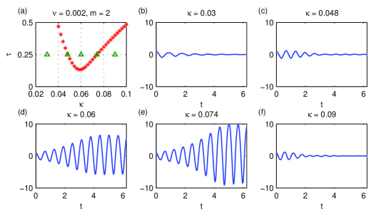
Figure 8: (a) Ince-Strutt diagram for $\displaystyle m=2$ and $\displaystyle\nu=0.002$ but with varying $\displaystyle\kappa$. The parameters used are denoted by $\displaystyle\triangle$, with the centre point corresponding to case 2. (b)–(f) Radial projection from simulations for a range of $\displaystyle\kappa$ values. The membrane was initialised with a $\displaystyle(2,0)$-mode and all curves are rescaled to start at $\displaystyle\widehat{X}^{r}=1$.

Finally, we show in figure 9 plots of the radial amplitude projection in cases 1–4, perturbing the spherical shell in each case with a mode that we know from the analysis to be unstable. The forcing amplitude is set to $\displaystyle\tau=0.45$ in all four cases. Snapshots of the membrane evolution are also given for each simulation to illustrate the growth of the given modes. All simulations exhibit the expected unstable growth in solution amplitude, although we stress that the numerical results do not lead to unbounded growth (or blow-up) in the amplitude as suggested by the linear analysis. We attribute this discrepancy in behaviour to nonlinear effects that become important later in the simulation and limit the solution growth when the amplitude of oscillations become large enough. We also note that the correct frequency response is observed in all four tests, with cases 1–3 exhibiting the expected period-doubling subharmonic response, while case 4 oscillates with a harmonic response.

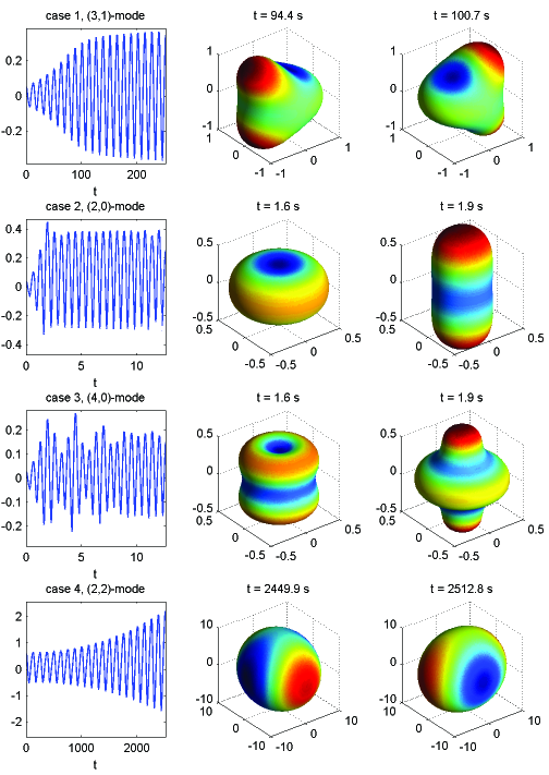
Figure 9: Simulation results for all four cases where a spherical shell perturbed by a mode that is expected to be unstable, with $\displaystyle\tau=0.45$. The left column shows the radial projection $\displaystyle\widehat{X}^{r}$, while snapshots from the corresponding simulations are shown on the right.

6 Application to the heart and other biofluid systems

Our work on parametric forcing of immersed elastic shells was originally motivated by the study of actively-beating heart muscle fibres that interact with surrounding blood and tissue. Heart muscle contractions are actually initiated by complex waves of electrical signals that propagate through the heart wall, which should be contrasted with the spatially-uniform coordinated contractions analysed in this paper. Furthermore, the heart chambers have an irregular shape and a thick wall that differ significantly from a spherical shell with zero thickness. Nonetheless, it is natural to ask whether our analysis of spherical immersed elastic shells with a periodic internal forcing could still yield any useful insights into the nature of the complex fluid-structure interaction between a beating heart and the surrounding fluid.

To this end, we consider an immersed spherical shell with parameters that correspond to the human heart under two conditions: first, a normal healthy heart; and second, an abnormal heart undergoing a much faster heartbeat. We then ask whether our analysis gives rise to resonant behaviour in either case for physiologically relevant heart beat frequencies. There are a wide range of abnormal heart rhythms classified under the heading of supraventricular tachycardia or SVT (Link, 2012; Phillips & Feeney, 1973), corresponding to a heart rhythm that is either irregular or abnormally rapid and occurs in the heart’s upper chambers (called the left and right atria). In contrast with ventricular tachycardias, which are much more dangerous, many SVTs are non-life-threatening and can persist for long periods of time. Therefore, we will focus on SVTs (and the atria) where fluid dynamic instabilities are more likely to have the time to develop.

We next discuss the choice of parameters that is appropriate for applying our IB model to study FSI in the heart. The resting heart rate for a healthy person ranges from 60 to 100 beats per minute (bpm) and both atria and ventricles beat in synchrony. In contrast, a heart characterised by SVT can exhibit two separate beats in the atria and ventricles, and can have an atrial rhythm that lies anywhere between 100 to 600 bpm. A clinical study by Wang et al. (2011) surveyed 322 patients suffering from atrial fibrillation (one sub-class of SVT) and obtained measurements of atrial wall stiffness $\displaystyle\sigma$ varying between $\displaystyle 1\times 10^{3}$ and $\displaystyle 2\times 10^{4}\;\mbox{$\displaystyle\mathrm{dyn/cm}$}$. We have found no evidence to suggest that the stiffness varies significantly between hearts with normal and abnormal rhythms, and so we use the same range of $\displaystyle\sigma$ for all cases. Although hearts suffering from conditions such as atrial fibrillation are often characterised by an increased size (Wang et al., 2011), we elect to use a single representative value of the radius $\displaystyle R=2.0\;\mbox{$\displaystyle\mathrm{cm}$}$ for an atrium in both normal and diseased hearts. In terms of the fluid properties, blood has density similar to water with $\displaystyle\rho=1\;\mbox{$\displaystyle\mathrm{g/cm^{3}}$}$ but has a significantly higher dynamic viscosity of $\displaystyle\mu=0.04\;\mbox{$\displaystyle\mathrm{g/cm\,s}$}$. We then choose a representative SVT rhythm with frequency $\displaystyle\omega=400$ bpm, which translates into a dimensionless viscosity parameter $\displaystyle\nu=2.39\times 10^{-4}$.

Substituting the parameter values and ranges just described into our analytical results from section 4 for the first three modes numbered $\displaystyle m=2,3,4$, we obtain the Ince-Strutt plot in figure 10. The stability fingers are depicted with the elastic stiffness parameter $\displaystyle\sigma$ plotted along the horizontal axis, and the results show that parametric instabilities can arise for most values of $\displaystyle\sigma$ under consideration. Because these resonant instabilities occur over such a wide range of stiffness values covered by the measurements by Wang et al. (2011) from the left atrium, it is reasonable to hypothesise that it may be possible for FSI-driven parametric instability to influence the dynamics of the beating heart.

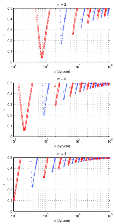
Figure 10: Stability contours for physical parameters corresponding to a human heart undergoing an abnormal heart rhythm ($\displaystyle\nu=2.39\times 10^{-4}$) for modes $\displaystyle m=2$ (top), 3 (middle) and 4 (bottom).

We now delve further into the finger plots in figure 10 and remark that experiments suggest the heart muscle is seldom (if ever) completely slack; therefore, we expect that the forcing amplitude parameter $\displaystyle\tau$ lies significantly below the threshold value of $\displaystyle\textstyle\frac{1}{2}$. Indeed, an estimate of $\displaystyle\tau\approx 0.3$ can be extracted from measurements of pressure in the left atrium taken by Braunwald et al. (1961, Fig. 1). Figure 11 provides an alternate view of the dependence of resonant instabilities on the parameters by depicting the minimum $\displaystyle\tau$ giving rise to resonance for as a function of elastic stiffness and beat frequency (using modes in the range $\displaystyle m=2$–6). We are especially interested in the dark (blue) bands that correspond to smaller values of $\displaystyle\tau$ and hence more prominent instabilities. Taking a value of $\displaystyle\tau=0.3$, our analysis predicts “valleys” of instability corresponding to discrete ranges of the parameters $\displaystyle\omega$ and $\displaystyle\sigma$. For fixed $\displaystyle\sigma$, we observe that at low frequency these valleys are very narrow and steep, while as the forcing frequency increases the width of the unstable bands likewise increases. In particular, if we consider an intermediate value of $\displaystyle\sigma$ for “normal” heart beating in the range of 60–100 $\displaystyle\mathrm{bpm}$, then the unstable bands are relatively small and so resonances would seem to be less likely. On the other hand, if the frequency is increased to 300–600 $\displaystyle\mathrm{bpm}$ then we begin to encounter wider valleys that suggest instabilities for a smaller value of $\displaystyle\tau$.

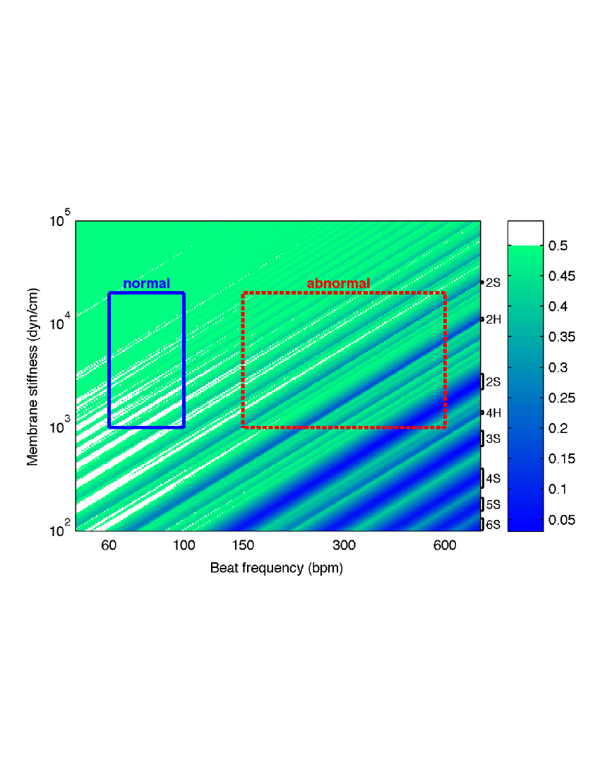
Figure 11: Minimum value of $\displaystyle\tau$ required for parametric resonance across modes 2–6. White areas represent parameters for which no physical instability exists. Each dark (blue) band is labelled by its corresponding unstable $\displaystyle m$-mode and response frequency (‘H’ for harmonic or ‘S’ for subharmonic). The boxes indicate parameter ranges for a healthy heart (solid, blue) and for a heart with SVT (dashed, red).

In summary, we have found that resonant instabilities are possible for a wide range of parameters corresponding to both normal and abnormal hearts; furthermore, for higher frequencies corresponding to SVT, instabilities are not only more likely to occur but also persist over wider ranges of parameter space. As suggestive as these results are, we refrain from making any specific claims or predictions regarding resonance in the actual beating heart since we have made so many simplifications and assumptions here: the applied periodic forcing is oversimplified, nonlinearities are neglected, a spherical shell is a far cry from an atrium, and parameter values are still quite uncertain. Nonetheless, the fact that our analysis predicts resonances for such a wide range of physiologically relevant parameters is compelling enough to suggest that this problem merit further investigation. Moreover, it should be possible to test for the presence of isolated parametric instabilities in carefully designed experiments, and our parameter study above provides guidance in what ranges of parameters are most worthy of investigation.

In addition to the heart, there are many other complex bio-fluid systems that undergo similar periodic internal forcing and for which our analytical results could potentially be applied. Parametric forcing in spherical membranes occurs in the context of dielectric characterisation and manipulation of biological cells (namely, erythrocytes and lymphocytes) by way of an applied electric field (Zehe & Ramírez, 2004). Another problem with spherical geometry was considered by Cottet et al. (2006), who were motivated by the study of cell membrane protrusions appearing in the process of cell locomotion. A much simpler geometry in which we have already applied a similar Floquet analysis is an IB model for the basilar membrane in the inner ear (Ko & Stockie, 2014). This problem involved a flat membrane for which the Floquet expansion takes a correspondingly simpler form in terms of trigonometric eigenfunctions. We showed that parametric resonances may play a significant role in the astounding ability of the mammalian ear to sense and process sound.

Another common geometry that is intermediate in complexity between the flat membrane and spherical shell is a cylindrical tube, which plays a central role in many biological structures (such as arteries, or bronchi in the lungs) as well as in engineering systems (involving compliant pipes or tubes). Indeed, there are many examples of FSI systems involving flow through a compliant cylindrical tube wherein some form of periodic forcing is known to induce resonance, including blood flow through artery-organ systems (Wang et al., 1991), air flow-induced vibrations of the bronchi (Grotberg, 1994), and the resonant impedance pump (Avrahami & Gharib, 2008; Loumes et al., 2008) whose design was incidentally inspired by observations of resonant pumping in the embryonic heart. An exciting possible avenue for future work is to extend our Floquet-type analysis to a cylindrical shell, which could then provide new insight into parametric resonance instabilities arising in these other FSI systems. One obvious advantage to studying this cylindrical geometry is that we can avoid the complexity of vector spherical harmonics and instead employ a simpler Floquet series solution consisting of Fourier-Bessel eigenfunctions, similar to the 2D radial solution obtained for a circular membrane in Cortez et al. (2004).

7 Conclusions

In this paper, we have demonstrated the existence of parametric instabilities in a spherical elastic shell immersed in an incompressible viscous fluid, wherein the motion is driven by periodic contractions of the shell. A mathematical model was derived using an immersed boundary framework that captures the full two-way interaction between the elastic material and the surrounding fluid. A Floquet analysis of the linearised governing equations is performed using an expansion in terms of vector spherical harmonics. We obtained results regarding the stability of the internally forced system with and without viscosity, and showed with the aid of Ince-Strutt diagrams that fluid-mechanical resonance exists regardless of whether viscous damping is present. Numerical simulations of the full IB model were performed that confirm the presence of these parametric resonances. In parallel with this work, we have initiated an experimental study of rubber water balloons immersed in water (Ko et al., 2014) in which we measure the natural modes of oscillation of these immersed (nearly-spherical) membranes and use the results to further validate our analytical predictions.

Because our original motivation for considering this problem derived from the study of periodic contractions driving blood flow in the heart, we also discussed the relevance of our stability analysis to cardiac fluid dynamics. Indeed, our analysis suggests that periodic resonances can occur in an idealised spherical shell geometry for physical parameters corresponding to the heart, provides possible parameter ranges to investigate in an experimental study that could test for resonant solutions. These results are very preliminary and much more work needs to be done to determine whether fluid-structure driven resonances can actually play a role in cardiac flows.

One major step in bringing our results closer to the actual heart is to generalise our time-periodic (but spatially uniform) driving force to include the effect of spiral waves of contraction that are initiated through electrical signals propagating in the heart wall. Including such spatiotemporal variations in the driving force would naturally couple together the radial and angular solution components. As a result, we would then lose the special advantage we gained from our choice of vector spherical harmonics that led to a fortunate mode-decoupling in the interfacial jump conditions. Generalising the analysis to handle this fully coupled problem would require a considerable effort, but could lead to significant new insights into a more realistic model of FSI in the beating heart.

Thanks go to Jeffrey Wiens for permitting us to use his immersed boundary code, as well as for providing assistance with the modifications required to perform the simulations in this paper. Financial support for this work came from a Discovery Grant and a Discovery Accelerator Award from the Natural Sciences and Engineering Research Council of Canada.

References

- Abramowitz & Stegun (1965) Abramowitz, M. & Stegun, I. A. 1965 Handbook of Mathematical Functions With Formulas, Graphs and Mathematical Tables. New York: Dover Publications.
- Avrahami & Gharib (2008) Avrahami, I. & Gharib, M. 2008 Computational studies of resonance wave pumping in compliant tubes. J. Fluid Mech. 608, 139–160.
- Barrera et al. (1985) Barrera, R., Estevez, G. & Giraldo, J. 1985 Vector spherical harmonics and their application to magnetostatics. Euro. J. Phys. 6, 287–294.
- Braunwald et al. (1961) Braunwald, E., Brockenbrough, E. C., Frahm, C. J. & Ross, Jr., J. 1961 Left atrial and left ventricular pressures in subjects without cardiovascular disease: Observations in eighteen patients studied by transseptal left heart catheterization. Circulation 24, 267–269.
- Champneys (2009) Champneys, A. R. 2009 The dynamics of parametric excitation. In Encyclopedia of Complexity and Systems Science (ed. Robert A. Meyers), pp. 183–204. Springer.
- Cortez et al. (2004) Cortez, R., Peskin, C. S., Stockie, J. M. & Varela, D. 2004 Parametric resonance in immersed elastic boundaries. SIAM J. Appl. Math. 65 (2), 494–520.
- Cortez & Varela (1997) Cortez, R. & Varela, D. 1997 The dynamics of an elastic membrane using the impulse method. J. Comput. Phys. 138 (1), 224–247.
- Cottet & Maitre (2006) Cottet, G. & Maitre, E. 2006 A level set method for fluid-structure interactions with immersed surfaces. Math. Models Meth. Appl. Sci. 16 (3), 415–438.
- Cottet et al. (2006) Cottet, G., Maitre, E. & Milcent, T. 2006 An Eulerian method for fluid-structure coupling with biophysical applications. In Proc. Euro. Conf. Comput. Fluid Dyn. (ECCOMAS CFD 2006) (ed. P. Wesseling, E. Oñate & J. Périaux). Egmond aan Zee, The Netherlands.
- Felderhof (2014) Felderhof, B. U. 2014 Jittery velocity relaxation of an elastic sphere immersed in a viscous incompressible fluid. Phys. Rev. E 89, 033001.
- Givelberg (2004) Givelberg, E. 2004 Modeling elastic shells immersed in fluid. Commun. Pure Appl. Math. 57 (3), 283–330.
- Grotberg (1994) Grotberg, J. B. 1994 Pulmonary flow and transport phenomena. Annu. Rev. Fluid Mech. 26, 529–571.
- Gunawan et al. (2005) Gunawan, A. Y., Molenaar, J. & van de Ven, A. A. F. 2005 Does shear flow stabilize an immersed thread? Euro. J. Mech. B 24, 379–396.
- Hill (1954) Hill, E. L. 1954 The theory of vector spherical harmonics. Amer. J. Phys. 22 (4), 211.
- Huang & Sung (2009) Huang, W. & Sung, H. J. 2009 An immersed boundary method for fluid–flexible structure interaction. Comput. Meth. Appl. Mech. Eng. 198 (33-36), 2650–2661.
- Kelly (1965) Kelly, R. E. 1965 The flow of a viscous fluid past a wall of infinite extent with time-dependent suction. Quart. J. Mech. Appl. Math. 18 (3), 287–298.
- Kleinstreuer (2006) Kleinstreuer, C. 2006 Biofluid Dynamics: Principles and Selected Applications. Boca Raton: CRC Press.
- Ko & Stockie (2014) Ko, W. & Stockie, J. M. 2014 An immersed boundary model of the cochlea with parametric forcing. SIAM J. Appl. Math. Under revision.
- Ko et al. (2014) Ko, W., Tse, D. & Stockie, J. M. 2014 Natural oscillations of a water balloon immersed in fluid. In preparation.
- Kumar & Tuckerman (1994) Kumar, K. & Tuckerman, L. S. 1994 Parametric instability of the interface between two fluids. J. Fluid Mech. 279, 49–68.
- Lai & Li (2001) Lai, M. & Li, Z. 2001 A remark on jump conditions for the three-dimensional Navier-Stokes equations involving an immersed moving membrane. Appl. Math. Lett. 14, 149–154.
- Lamb (1932) Lamb, H. 1932 Hydrodynamics. Cambridge University Press.
- Lighthill (1975) Lighthill, Sir J., ed. 1975 Mathematical Biofluiddynamics, CBMS-NSF Regional Conference Series in Applied Mathematics, vol. 17. Philadelphia: SIAM.
- Link (2012) Link, M. S. 2012 Evaluation and initial treatment of supraventricular tachycardia. New Engl. J. Med. 367, 1438–1448.
- Loumes et al. (2008) Loumes, L., Avrahami, I. & Gharib, M. 2008 Resonant pumping in a multilayer impedance pump. Phys. Fluids 20, 023103.
- Morse & Feshbach (1953) Morse, P. M. & Feshbach, H. 1953 Methods of Theoretical Physics, Part II. New York: McGraw-Hill.
- Nayfeh (1993) Nayfeh, A. H. 1993 Introduction to Perturbation Techniques. New York: John Wiley & Sons.
- Persson & Strang (2004) Persson, P. & Strang, G. 2004 A simple mesh generator in Matlab. SIAM Rev. 46, 329–345.
- Peskin (1977) Peskin, C. S. 1977 Numerical analysis of blood flow in the heart. J. Comput. Phys. 25, 220–252.
- Peskin (2002) Peskin, C. S. 2002 The immersed boundary method. Acta Numer. pp. 1–39.
- Phillips & Feeney (1973) Phillips, R. E. & Feeney, M. K. 1973 The Cardiac Rhythms: A Systematic Approach to Interpretation. Philadelphia, PA: Saunders.
- Ramanujan & Pozrikidis (1998) Ramanujan, S. & Pozrikidis, C. 1998 Deformation of liquid capsules enclosed by elastic membranes in simple shear flow: large deformations and the effect of fluid viscosities. J. Fluid Mech. 361, 117–143.
- Semler & Païdoussis (1996) Semler, C. & Païdoussis, M. P. 1996 Nonlinear analysis of the parametric resonances of a planar fluid-conveying cantilevered pipe. J. Fluids Struct. 10, 787–825.
- Stockie & Wetton (1995) Stockie, J. M. & Wetton, B. T. R. 1995 Stability analysis for the immersed fiber problem. SIAM J. Appl. Math. 55 (6), 1577–1591.
- Terzopoulos & Fleischer (1988) Terzopoulos, D. & Fleischer, K. 1988 Deformable models. Visual Computer 4 (6), 306–331.
- Vogel (1994) Vogel, S. 1994 Life in Moving Fluids: The Physical Biology of Flow, 2nd edn. Princeton University Press.
- Wang et al. (2011) Wang, W., Buehler, D., Martland, A. M., Feng, X. D. & Wang, Y. J. 2011 Left atrial wall tension directly affects the restoration of sinus rhythm after Maze procedure. Eur. J. Cardiothorac. Surg. 40 (1), 77–82.
- Wang et al. (1991) Wang, Y. Y. L., Chang, S. L., Wu, Y. E., Hsu, T. L. & Wang, W. K. 1991 Resonance: The missing phenomenon in hemodynamics. Circ. Res. 69, 246–249.
- Wiens (2014) Wiens, J. K. 2014 An efficient parallel immersed boundary algorithm, with application to the suspension of flexible fibers. PhD thesis, Department of Mathematics, Simon Fraser University.
- Wiens & Stockie (2014) Wiens, J. K. & Stockie, J. M. 2014 An efficient parallel immersed boundary algorithm using a pseudo-compressible fluid solver. J. Comput. Phys. To appear, arXiv:1305.3976.
- Zehe & Ramírez (2004) Zehe, A. & Ramírez, A. 2004 Vibration of eukariotic cells in suspension induced by a low-frequency electric field: A mathematical model. Trans. Biol. Biomed. 1 (1), 55–59.