Lattice Three-Dimensional Skyrmions Revisited

E.G. Charalampidis${}^{1,2^{*}}$,  T.A. Ioannidou${}^{1^{\dagger}}$  and   P.G. Kevrekidis${}^{2^{\ddagger}}$

¹School of Civil Engineering, Faculty of Engineering, Aristotle University of Thessaloniki,
54124 Thessaloniki, Greece
²Department of Mathematics and Statistics, University of Massachusetts, Amherst,
Massachusetts 01003-4515, USA

In the continuum a skyrmion is a topological nontrivial map between Riemannian manifolds, and a stationary point of a particular energy functional. This paper describes lattice analogues of the aforementioned skyrmions, namely a natural way of using the topological properties of the three-dimensional continuum Skyrme model to achieve topological stability on the lattice. In particular, using fixed point iterations, numerically exact lattice skyrmions are constructed; and their stability under small perturbations is explored by means of linear stability analysis. While stable branches of such solutions are identified, it is also shown that they possess a particularly delicate bifurcation structure, especially so in the vicinity of the continuum limit. The corresponding bifurcation diagram is elucidated and a prescription for selecting the branch asymptoting to the well-known continuum limit is given. Finally, the robustness of the spectrally stable solutions is corroborated by virtue of direct numerical simulations .

^∗ Email: echarala@auth.gr

^† Email: ti3@auth.gr

^‡ Email: kevrekid@math.umass.edu

1 Introduction

Lattice models involve discrete systems where the motion of a lattice particle depends on and also affects the motion of its neighbors. When considering the long wavelength approximation of the discrete system, the latter is transformed into a continuum medium for which partial differential equations govern the local motion; see e.g. [1]-[4] for some case examples. Many attempts have been made in order to find methods that faithfully represent the continuum limits of discrete models or vice versa that accurately capture the continuum phenomenology within the discrete case (the latter is also relevant, in the context of numerical computation). For a given continuum model, there are many different discrete analogues which reduce to it in the continuum limit.

In [5] a scheme was proposed for generating one-dimensional topological lattice systems. It maintains an important feature of the continuum model, namely the topological lower bound (so-called, Bogomolny bound) of the energy; while the lattice solitons saturate this lower bound. These are solutions of the lattice Bogomolny equation. However, an open issue is whether topology and topological stability of the solitons can be maintained on the lattice. In the continuum, the stability of the topological solitons is often related to the existence of such an energy bound but in the lattice, it is not clear whether the corresponding topological objects are also stable. The discretization scheme of [5] has been applied in few continuum theories which have a Bogomolny bound [6]-[10]; but also used in non-topological systems where a Bogomolny-type argument can be applied [11]. The aforementioned features are not preserved in two-dimensional systems, since the energy of the lattice solitons is greater than the topological minimum [12].

In this paper, following [5], a lattice version of the Skyrme model in $3+1$ dimensions is described based on a Bogomolny-type argument. To do so we impose radial symmetry on the field, thus a one-dimensional system is obtained, and then its lattice version which maintains a Bogomolny-type bound is presented. A similar study, has been applied for studying the properties of the $Q$-balls defined at the continuum [11]. The corresponding results were obtained analytically and were close to the exact ones obtained by solving the full equations numerically.

The three-dimensional Skyrme model [13] serves as a popular model of the dynamics of pions and nucleons, incorporating the former as its fundamental pseudo-Goldstone field and the latter in the form of topological solitons. Its lattice formulation is of some importance in its own right. The model is non-renormalizable in perturbation theory and existing treatments of the model are semiclassical (quantizing only the collective degrees of freedom of the soliton). A full quantization of the theory requires a cutoff which can be attained by its lattice version.

2 The Lattice Skyrme Model

The Lagrangian density of the Skyrme model is of the form

$$12\pi^{2}{\cal L}=-\frac{1}{2}{\rm tr}\left(R_{\mu}R^{\mu}\right)+\frac{1}{16}{\rm tr}\left(\left[R_{\mu},R_{\nu}\right]\left[R^{\mu},R^{\nu}\right]\right),$$ (2.1)

where $R_{\mu}=\partial_{\mu}UU^{-1}$, the indices $\mu,\nu$ run from $0$ to $3$ and the metric is the Minkowski one, i.e.: $g_{\mu\nu}=\mbox{diag}(1,-1,-1,-1)$ and $U$ is the $SU(N)$ Skyrme field. In order for finite energy field configurations to exist, the Skyrme field $U$ has to tend to a constant matrix at spatial infinity. This compactifies the domain space of the Skyrme field $U$ into a large three-sphere and, thus, the static solutions are maps from $S^{3}\mapsto SU(N)$ and as such can be classified by an integer-valued degree, (the so-called, topological charge or baryon number), denoted by $B$. Therefore a skyrmion is a finite energy field configuration corresponding to topological solitons and carrying topological charge $B$.

In [14], a separation of variables ansatz was introduced for the Skyrme field by decomposing it into a radial and an azimuthal part. The former is captured by a real profile function, namely $f(r)$ and the latter by a Hermitian projector $P$ that depends only on the angular variables.

Then, the kinetic and potential energy of the Skyrme model are equal to

$$E_{\mbox{\tiny kin}} = \frac{1}{3\pi}\int\dot{f}^{2}\left(A_{N}r^{2}+2{\cal N}\sin^{2}{f}\right)dr,$$

$$E_{\mbox{\tiny pot}} = \frac{1}{3\pi}\int\left(A_{N}r^{2}f_{r}^{2}+2{\cal N}\left(f_{r}^{2}+1\right)\sin^{2}{f}+{\cal I}\,\frac{\sin^{4}{f}}{r^{2}}\right)dr,$$ (2.2)

respectively. Here, ${\cal N}$, ${\cal I}$ and $A_{N}$, are parameters independent of the radial variable $r$, integrals of functions of $P$ (for details, see [10] and references therein); while $f(0)=\pi$ due to well posedness of (2.1) and $f(\infty)=0$ due to energy finiteness. The Skyrme model has no Bogomolny bound; however, a Bogomolny-type argument leads to the bound

$$E_{\mbox{\tiny pot}}\!\!\! \!\!\!=\!\!\! \!\!\!\frac{1}{3\pi}\!\int\!\!\left\{\left(\sqrt{A_{N}}f_{r}r+\sqrt{\cal I}\frac{\sin^{2}{f}}{r}\right)^{2}\!\!+2{\cal N}\sin^{2}{f}(1+f_{r})^{2}+2(2{\cal N}+\sqrt{A_{N}{\cal I}})\sin{f}\partial_{r}(\cos{f})\right\}dr$$ (2.3)

$$\geq \frac{1}{3}(2{\cal N}+\sqrt{A_{N}{\cal I}}),$$

which is stronger than the usual Fadeev-Bogomolny one $E_{\mbox{\tiny pot}}\geq 12\pi^{2}{B}$. Thus the discretization scheme of [5] can be applied in order to examine whether the corresponding lattice skyrmions are stable.

In [10], based on such a Bogomolny-type argument, a discretization scheme was applied to derive spherically symmetric three-dimensional skyrmions. However, an unfortunate sign error was present in the latter calculation that has been corrected herein. In order to obtain an appropriate discrete version of the Skyrme model, there are two critical points to be considered: a) the discretization formulae of the Skyrme fields and corresponding terms and b) the choice of the discrete potential energy at the origin. In this note, both forms have been accounted for appropriately in order to obtain a relevant result addressed below.

Hereafter, $r$ becomes a discrete variable with lattice spacing $h$ while the real-valued field $f(r,t)$ depends on the continuum variable $t$ and the variable $r=nh$ where $n\in Z^{+}$. Then, $f_{+}=f\left((n+1)h,t\right)$ denotes a forward shift and thus, the forward difference is given by $\Delta f=(f_{+}-f)/h$. To obtain a lattice version of the Bogomolny-type bound, we start with the last term of (2.3) and discretize it as: $\sin f\partial_{r}(\cos f)=\sin f\Delta(\cos f)\equiv-\frac{2}{h}\sin f\sin\left(\frac{f_{+}-f}{h}\right)\sin\left(\frac{f_{+}+f}{h}\right)$. This leads to the following discretization choices:

$$f_{r} \rightarrow \frac{2}{h}\,\sin\left(\frac{f_{+}-f}{2}\right),$$

$$\sin f \rightarrow \sin\left(\frac{f_{+}+f}{2}\right).$$ (2.4)

The same discretization scheme can be applied at the origin with the only assumption that at the origin the Bogomolny-type equation is satisfied, i.e. $\sqrt{A_{N}}f_{r}r+\sqrt{\cal I}\frac{\sin^{2}{f}}{r}\equiv 0$. Thus, the discrete kinetic and potential energy assume the form:

$$E_{\mbox{\tiny kin}}\!\!\!\! = \!\!\!\!4\pi h\sum_{n=1}^{\infty}\left[A_{N}\,n^{2}h^{2}+2{\cal N}\sin^{2}\left(\frac{f_{+}+f}{2}\right)\right]\dot{f}^{2},$$ (2.5)

$$E_{\mbox{\tiny pot}}\!\!\!\! = \!\!\!\!8\pi h\,\cos^{2}\left(\frac{f_{1}}{2}\right)\left[{\cal N}\left(\frac{4}{h^{2}}\,\cos^{2}\left(\frac{f_{1}}{2}\right)+1\right)+\frac{2}{h}\sqrt{A_{N}{\cal I}}\cos\left(\frac{f_{1}}{2}\right)\right]$$

$$+ \!\!\!\!4\pi h\sum_{n=1}^{\infty}\Bigg{\{}4A_{N}n^{2}\sin^{2}\left(\frac{f_{+}-f}{2}\right)+\frac{{\cal I}}{n^{2}h^{2}}\sin^{4}\left(\frac{f_{+}+f}{2}\right)+2{\cal N}\left[\frac{4}{h^{2}}\sin^{2}\left(\frac{f_{+}-f}{2}\right)+1\right]\sin^{2}\left(\frac{f_{+}+f}{2}\right)\Bigg{\}}.$$

Then, the Euler-Lagrange equations read

$$\ddot{f}\left[A_{N}h^{2}+2{\cal N}\sin^{2}\left(\frac{f_{+}+f}{2}\right)\right]+{\cal N}\dot{f}\left(\dot{f}_{+}+\dot{f}\right)\sin{\left(f_{+}+f\right)}-\frac{\cal N}{2}\dot{f}^{2}\sin\left(f_{+}+f\right)$$

$$=\frac{\sin{f_{1}}}{2h^{2}}\left[3h\sqrt{A_{N}{\cal I}}\cos{\left(\frac{f_{1}}{2}\right)}+{\cal N}\left(8\cos^{2}{\left(\frac{f_{1}}{2}\right)}+h^{2}\right)\right]$$

$$+A_{N}\sin(f_{+}-f)-\frac{{\cal I}}{2h^{2}}\sin{\left(f_{+}+f\right)}\sin^{2}{\left(\frac{f_{+}+f}{2}\right)}$$

$$+\frac{{\cal N}}{2}\left[\frac{4}{h^{2}}\sin{\left(f_{+}-f\right)}\sin^{2}{\left(\frac{f_{+}+f}{2}\right)}-\sin{\left(f_{+}+f\right)}\left(\frac{4}{h^{2}}\sin^{2}{\left(\frac{f_{+}-f}{2}\right)}+1\right)\right],\hskip 14.22636ptn=1,$$

$$\ddot{f}\left[A_{N}n^{2}h^{2}+2{\cal N}\sin^{2}\left(\frac{f_{+}+f}{2}\right)\right]+{\cal N}\dot{f}\left(\dot{f}_{+}+\dot{f}\right)\sin{\left(f_{+}+f\right)}$$

$$-\frac{{\cal N}}{2}\left[\dot{f}^{2}\sin{\left(f_{+}+f\right)}+\dot{f}_{-}^{2}\sin{\left(f+f_{-}\right)}\right]$$

$$=A_{N}n^{2}\sin(f_{+}-f)-A_{N}(n-1)^{2}\sin(f-f_{-})$$

$$+\frac{{\cal N}}{2}\left[\frac{4}{h^{2}}\sin{\left(f_{+}-f\right)}\sin^{2}\left(\frac{f_{+}+f}{2}\right)-\sin{\left(f_{+}+f\right)}\left(\frac{4}{h^{2}}\sin^{2}{\left(\frac{f_{+}-f}{2}\right)}+1\right)\right]$$

$$-\frac{{\cal N}}{2}\left[\sin{\left(f+f_{-}\right)}\left(\frac{4}{h^{2}}\sin^{2}{\left(\frac{f-f_{-}}{2}\right)}+1\right)+\frac{4}{h^{2}}\sin{\left(f-f_{-}\right)}\sin^{2}\left(\frac{f+f_{-}}{2}\right)\right]$$

$$-\frac{\cal I}{2h^{2}}\left[\frac{\sin{\left(f_{+}+f\right)}}{n^{2}}\sin^{2}{\left(\frac{f_{+}+f}{2}\right)}+\frac{\sin{\left(f+f_{-}\right)}}{\left(n-1\right)^{2}}\sin^{2}{\left(\frac{f+f_{-}}{2}\right)}\right],\hskip 14.22636ptn>1.$$

(2.8)

In what follows we consider the $SU(2)$ case (where the Skyrme field $U$ is a mapping between three-spheres, since the $SU(2)$ group is isomorphic to $S^{3}$) and focus on the $B=1$ topological sector. This implies (see, also, [10]) that the corresponding parameters take the values of $A_{N}=1$, ${\cal N}={\cal I}=1$, respectively.

3 Numerical Simulations

In this section solutions of the Euler-Lagrange equations (LABEL:eor) and (2.8) are derived numerically by assuming a lattice consisting of $n_{\textrm{max}}=800$ nodes (unless explicitly stated otherwise). In particular, a fixed point iteration is used to identify relevant steady states and linear stability analysis is applied to study their response to small perturbations. Although two principal (and disconnected between them) branches of solutions are obtained and presented below, it turns out that only one tends smoothly towards the corresponding continuum limit of the system, as soon as $h\rightarrow 0$; see the relevant discussion below. Furthermore, the robustness of the solution segments of both branches which are found to be linearly stable is corroborated by direct numerical simulations of the time evolution dynamics.

The investigation consists of three parts: existence, stability and dynamics. Concerning the existence, the numerical procedure used is a Newton - Raphson algorithm accompanied by a suitable initial guess; in this way a static solution is obtained (up to a prescribed tolerance) after a few iterations. Note that at the origin (i.e., $n=0$), we impose explicitly the boundary condition $f(0)=\pi$ (i.e., we consider the case of compactified $R^{3}$ and not that of the compactified $R^{3}$ minus a small ball of radius $\delta$ around the origin, as the latter would not possess stable topological solitons even in the continuum limit). At the right end of the computational domain (i.e., $n=n_{\textrm{max}}+1$), a homogeneous Dirichlet boundary condition is applied, enforcing the existence of a topological lattice soliton.

In Fig. 1, the discrete profile function for various values of the lattice spacing $h$ is shown. In particular, panel (a) corresponds to $h=1$ (an example of a rather discrete case) while panels (b)-(e) correspond to $h=0.4,\ 0.4,\ 0.3$ and $0.2$ (examples gradually approaching the continuum case), respectively, and all labeled in connection with Fig. 3. As an initial guess, a profile with exponential decay of the form $f_{n}=\pi e^{-bnh}$ is used, where $b$ is a width-controlling parameter. It is obvious from the top panels of Fig. 1 that as $h$ decreases, the solution appears to naturally and smoothly converge to its continuum counterpart; nevertheless, as we will see below, this is not the branch that reaches the well-established continuum limit of the model, due to the delicate structure of the bifurcation diagram of this system. The latter limit is illustrated in the top right panel of Fig. 1 with blue solid line as computed via a collocation method (see, for details, [15]) applied to the corresponding ordinary differential equation [16], thus yielding its static radial topological soliton solution. Furthermore, although the profiles of panels (b) and (c) correspond to the same value of $h$($=0.4$), they differ not only structurally but the solution of panel (c) appears to be unstable according to the stability analysis that we will present next. Furthermore, we report the solutions of panels (d) and (e) which appear structurally and physically not to be related with the skyrmion of the continuum limit. In particular, these solutions are not only lacking the smoothness of the limit, but also the positive-definite structure of its profile. This is a feature that is not disallowed by our discretization, as $h\rightarrow 0$, given the angular nature of our variables and the sinusoidal nature of our associated discretization terms.

        

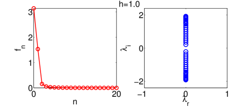
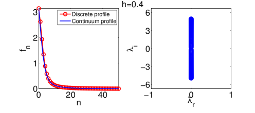
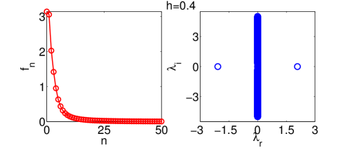
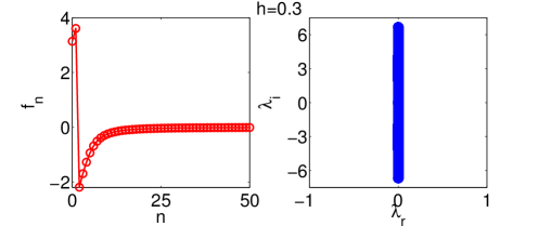
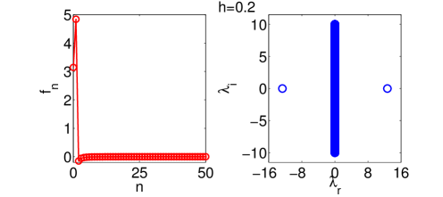
Figure 1: (Color online) Static discrete profiles and corresponding eigenvalue spectra for the first branch of solutions are presented for a value of the lattice spacing of (a) $h=1$ (with $n_{\textrm{max}}=19$), (b) $h=0.4$ (with $n_{\textrm{max}}=49$), (c) $h=0.4$, (d) $h=0.3$ and (e) $h=0.2$. These solutions correspond to the (a)-(e) labels of Fig. 3. In panel (b), the discrete (red circles) against the continuum (solid blue line) profile is plotted for comparison.

  

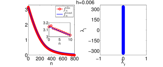
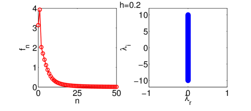
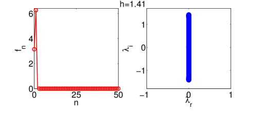
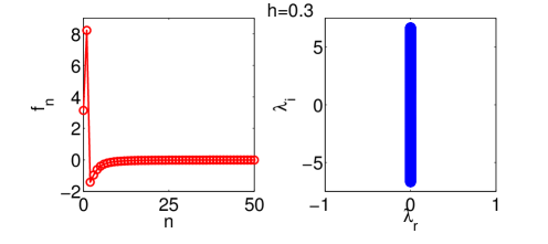
Figure 2: (Color online) Same as Fig. 1 but for the second branch of solutions. Static discrete profiles and corresponding eigenvalue spectra for a value of the lattice spacing of (a) $h=6\times 10^{-3}$, (b) $h=0.2$, (c) $h=1.41$ and (d) $h=0.3$. These solutions correspond to the (a)-(d) labels of Fig. 4. In panel (a), the discrete (red circles) against the continuum (solid blue line) profile is plotted for comparison.

Concerning the stability of the obtained lattice skyrmions the following analysis is used. A linearization scheme around the stationary point $f^{0}$ is employed, in order to study the effect of small perturbations. So, the profile function is chosen to be of the form:

$$f_{n}=f_{n}^{0}+\epsilon\exp{\left(\lambda t\right)}\,w_{n},\hskip 14.22636pt(\epsilon\ll 1).$$ (3.9)

That way, at order $O(\epsilon)$, an eigenvalue problem is obtained with $\left(\lambda,w_{n}\right)$ representing the corresponding eigenvalue and eigenvector, respectively. Then, the eigenvalues $\lambda=\lambda_{r}+i\lambda_{i}$ without a positive real part $\lambda_{r}$ correspond to oscillatory, marginally stable eigendirections (in our numerical computations presented below, we consider a steady state solution having $\textrm{Max}(\lambda_{r})<5\times 10^{-4}$ to be stable). For instance, the eigenvalue spectra shown in panels (a), (b) and (d) of Fig. 1 and panels (a)-(d) of Fig. 2 suggest that the corresponding solutions are dynamically stable since all the linearization eigenvalues are sitting on the imaginary axis. On the contrary, if the solution possesses either a real eigenvalue pair or a complex eigenvalue quartet (for the Hamiltonian problem at hand), this signals a dynamical instability with a growth rate provided by the real part of the corresponding eigenvalue. As it can be inferred from panels (c) and (e) of Fig. 1, the solutions turn out to be unstable characterized by a real eigenvalue pair.

Surprisingly, the solutions of Fig. 1 are not the only discrete solitons that exist. A second branch of discrete solitons exists that was traced through the Newton-Raphson method. Four examples of them are shown in panels (a)-(d) of Fig. 2 for $h=0.006,\ 0.2,\ 1.41$ and $0.3$, respectively. This branch of solutions is found to be linearly stable and specifically, for very small values of $h$, matches very closely the continuum limit of the topological soliton profile obtained through the collocation method. Nevertheless, some comments are due here.

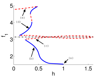
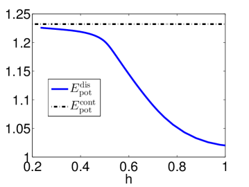
Figure 3: (Color online) Results of continuation over the spacing parameter for the first branch of solutions: (a) Plot of the static discrete profile at the first site of the domain as a function of the lattice spacing (i.e. $f_{1}(h)$). The solid (blue) segments correspond to stable regions while the dash-dotted (red) ones correspond to (real eigenvalue bearing) unstable parametric regions, respectively. Note that the horizontal dash-dotted black line corresponds to the value of $\pi$. (b) Plot of the normalized potential energy (i.e. $E_{\mbox{\tiny pot}}/12\pi^{2}$) of our static solution (blue) as a function of $h$. The dash-dotted (black) line corresponds to the actual value of the normalized continuum potential energy which is equal to 1.232.

Although this second branch of solutions appears to very accurately capture the continuum limit, the inset of Fig. 2 suggests a very slight mismatch near the origin (more precisely, at $n=1$). Admittedly, this disparity must be introduced by our special way of handling the $n=1$ site to avoid singularities in the discrete setting (cf. equation (2.8)). In order to understand the differences between these two branches, the characteristics of continuation of the obtained solutions over the lattice spacing $h$ (using the computer software AUTO [17, 18]) are displayed in Fig. 3 and the top row of Fig. 4, in terms of the value of the profile $f_{n}$ at $n=1$ (see, panels (a)) together with the corresponding total potential energy $E_{\textrm{pot}}$ (see, panels (b)) given by Eq. (2). These parametric continuations start from a large value of $h$ and, through progressive small decrements, tending towards the continuum limit of $h\rightarrow 0$, illustrate the distinction between the branches. However, when they encounter turning points, the pseudo-arclength nature of the continuation enables the code to bypass the relevant folds in the bifurcation diagram, allowing the visualization of the complex bifurcation pattern.

The first branch of Fig. 3 is initiated at the value of the lattice spacing of $h=1$ (see, Fig. 1 and label (a) in Fig. 3) and smoothly approaches the continuum limit as $h$ is decreased (see, Fig. 1 and label (b) in Fig. 3), as shown for the ordinate of the first site and also, for the potential energy of the solution depicted in Fig. 3. However, this first branch presents an intriguing feature: although it appears to asymptote smoothly towards the proper continuum counterpart, a saddle-node bifurcation at $h\approx 0.234$ appears, followed by a turning point (at $h\approx 1.597$) and an eventual cascade of saddle-node bifurcations (starting at $h\approx 0.115$), changing structurally the discrete profiles and the stability thereof. For the latter, it should be pointed out that stable and unstable regions are presented in Fig. 3 with solid blue and dash-dotted red lines, respectively. Furthermore, the solution branch labeled with (e) in Fig. 3 (see also panel (e) in Fig. 1) can be continued down for very small values of $h$, although the obtained solutions are unstable while the ordinate of the first site does not asymptote to the correct continuum limit. The lack of smoothness (a priori not disallowed by our discretization, as per the discussion above) and the lack of stability suggest that this continuation does not asymptote to the proper continuum limit solution. Nevertheless, this is remedied by the second branch of solutions that we now consider.

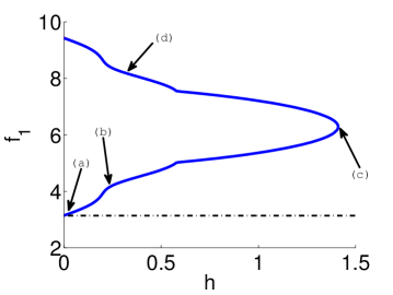
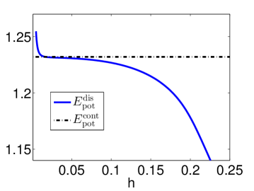
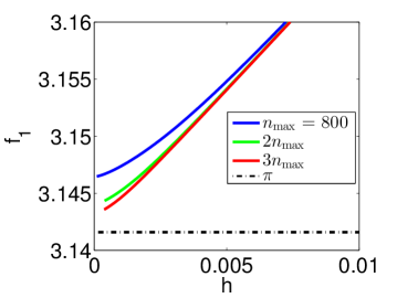
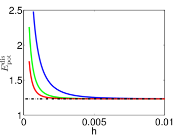
Figure 4: (Color online) Same as Fig. 2 but for the second branch of solutions. Panels (c) and (d) are zoomed-in versions of (a) and (b) where a direct comparison of the continuation results for values of $n_{\textrm{max}}=800$ (blue), $n_{\textrm{max}}=1600$ (green) and $n_{\textrm{max}}=2400$ (red), respectively, is shown.

Indeed, it was this inability to identify the correct continuum limit as $h\rightarrow 0$ that led us to the second branch of solutions presented in Figs. 2 and 4. This branch is not of the monotonic (profile) type as was the case in some parametric regions of the first one, although it is stable throughout the range of the lattice spacing $h$ considered. As shown in the top left panel of Fig. 4, the profile function of the first site is always $f_{1}>\pi$ (see also, panels (b)-(d) in Fig. 2) while the bottom segment labeled by (a) only approaches $\pi$ as $h\rightarrow 0$. This feature appears to be less physical and a particular attribute of the discretization imposed here for $n=1$. However, it can be smoothly continued to extremely small values of $h$ thus, approaching the corresponding continuum limit (as shown with the solid blue line in Fig. 4). In particular, at such small values of $h$ the precise (distinct from $n\neq 1$) form of the discrete equation for $n=1$ appears to be responsible for the induced jump (see the inset of Fig. 2) and also for the overshooting evident in the top right panel of Fig. 4. To investigate this issue further and confirm the approach of the proper continuum limit by the lower portion of this branch, we increased the total number of the nodes $n_{\textrm{max}}$ in the one-dimensional lattice. The bottom row of Fig. 4 summarizes our findings using $n_{\textrm{max}}=800,1600$ and $2400$ lattice nodes where panels (c) and (d) correspond to the zoom-ins of panels (a) and (b), respectively. It can be discerned from Fig. 4 that the trend of $f_{1}(h)$ gradually asymptotes to the correct continuum limit as the total number of the nodes is increased. The latter suggests that for a sufficiently “large” lattice we are able to recover the correct continuum radial profile, thus establishing the consistency of the discretization scheme (2.4) employed. Finally, the overshooting that appears in the discrete potential energy in Fig. 4 gradually disappears as shown in Fig. 4 for larger values of $n_{\textrm{max}}$, therefore enforcing the validity of the scheme proposed. Hence, clearly the lower portion of the second branch not only is smooth but also approaches a smooth, positive monotonic profile in the continuum limit, thereby properly asymptoting to the continuum soliton. However, it should be noted that this branch of solutions too, as $h$ is increased goes around a turning point; this implies that this family of solutions cannot be continued indefinitely within the highly discrete regime. Past this fold, the solution again acquires a non-smooth, non-sign-definite form, hence not being a suitable candidate for continuation towards the continuum limit. It is thus through the smoothness (and, in part, the positive-definiteness and the stability properties) of the solution that we select the suitable candidate (among the different available solutions for small $h$) for reaching the continuum limit.

Let us conclude by stating that solutions “living” in stable regions of both branches (and particularly those physically resembling the corresponding skyrmion in the continuum limit) are natural discrete representations of the corresponding topological solitary wave and, in fact, dynamically robust ones such. The latter is illustrated in more detail in Fig. 5 for solutions of the first branch and in Fig. 6 for those of the second one (in connection with the solutions in panels (a) and (b) of Figs. 1 and 2, respectively). Both figures confirm the dynamical stability of the obtained discrete solitons by testing the direct dynamical evolution of the system of equations (2.8) in the presence of small, random (uniformly distributed) perturbations imposed on top of the solitary wave. These perturbations lead solely to oscillations both in the kinetic and potential energy of the solutions –while their total energy remains very accurately conserved– and in the ordinate of the first site. To sum up, the solution does not structurally modify its form for either branch.

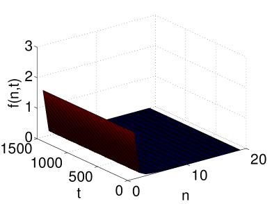
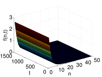
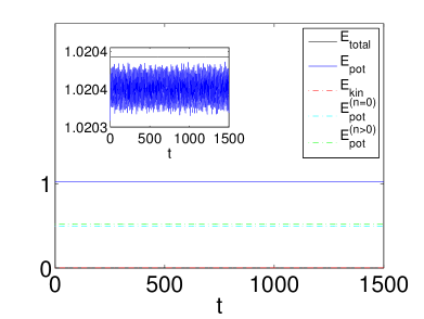
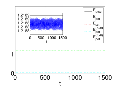
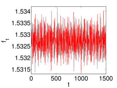
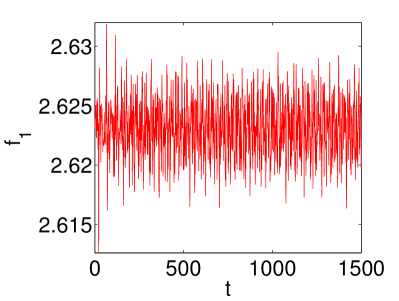
Figure 5: (Color online) Time evolution of the perturbed solutions of Fig. 1. Left and right panels correspond to lattice spacing $h=1$ and $h=0.4$, respectively. The top panels (a-b) show the space-time evolution of the profile function $f(n,t)$. The middle panels (c-d) illustrate the evolution of the kinetic and potential energies, and the conservation of the total energy. The bottom panels (e-f) show the dependence of the profile function $f_{1}$ versus time, upon the imposition of the small random perturbation.

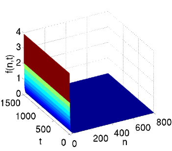
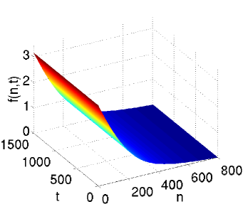
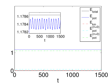
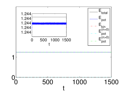
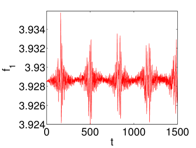
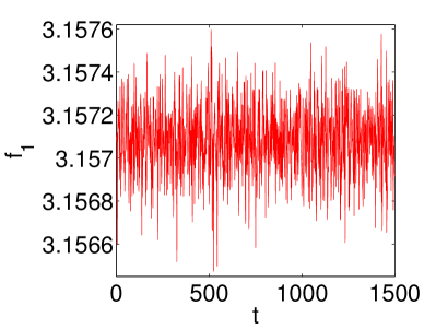
Figure 6: (Color online) Time evolution of the perturbed solutions of Fig. 2. Left and right panels correspond to values of the lattice spacing $h=0.2$ and $h=0.006$, respectively. The top panels (a-b) show the space-time evolution of the profile function $f(n,t)$. The middle panels (c-d) illustrate the evolution of the kinetic and potential energies, and the conservation of the total energy. The bottom panels (e-f) show the dependence of the profile function $f_{1}$ versus time, again in the presence of a small random initial perturbation.

4 Conclusions

In this brief communication, we have revisited the problem of three-dimensional skyrmions and the corresponding discretization of the radial continuum problem in order to pose it on a lattice setting (and therefore with a natural cutoff scale). We have presented a self-consistent form of the relevant discretization, amending the earlier work of [10] in that regard, as concerns the energy of the site which lies immediately next to the origin. This discretization has led to the identification of two principal branches of solutions in the form of discrete skyrmions, which both can be continued down for very small values of $h$. However, only one is smooth, positive definite and stable, becoming strongly reminiscent of the continuum limit. The approach to the limit is further investigated by gradually magnifying the radial domain, thus revealing the consistency of the radial discretization scheme employed. Interestingly, a fairly complex bifurcation diagram is revealed for both branches, including a number of turning points and saddle-node bifurcations. Then, solutions of both branches belonging to parametric regions which are found to be linearly stable (by eigenvalue computations within the realm of linear stability analysis) have been tested against direct numerical simulations under the presence of small perturbations.

While alternative discretizations of the radial $SU(2)$ Skyrme problem (potentially extended e.g. to the $SU(3)$ one) are of interest in their own right, the identification of discretizations of the axially symmetric problem, or even the fully three-dimensional one that possess stable discrete skyrmions that naturally approach their continuum siblings as the lattice spacing tends to zero, remains a broader problem of interest in its own right. Studies along this direction are currently in progress and will be reported in future publications.

Acknowledgements

The authors acknowledge support from FP7, Marie Curie Actions, People, International Research Staff Exchange Scheme (IRSES-605096). E.G.C. is indebted to the Institute of Physics, Carl von Ossietzky University (Oldenburg) for the kind hospitality provided while part of this work was carried out and acknowledges financial support from the German Research Foundation DFG, the DFG Research Training Group 1620 “Models of Gravity”. T.A.I. also acknowledges support from The Hellenic Ministry of Education: Education and Lifelong Learning Affairs, and European Social Fund: NSRF 2007-2013, Aristeia (Excellence) II (TS-3647). P.G.K. also acknowledges support from the National Science Foundation under grants CMMI-1000337, DMS-1312856, from the Binational Science Foundation under grant 2010239 and from the US-AFOSR under grant FA9550-12-10332.

References

- [1] M. Remoissenet, Waves called solitons (Springer, Berlin, 1999).
- [2] V.F. Nesterenko, Dynamics of Heterogeneous Materials, Springer-Verlag (New York, 2001).
- [3] T. Dauxois and M. Peyrard, Physics of Solitons, Cambridge University Press, (Cambridge, 2006).
- [4] T. Ioannidou, J. Pouget and E. Aifantis, J. Phys. A 36 645 (2003); J. Phys. A 34 (2001) 4269.
- [5] J. M. Speight and R. S. Ward, Nonlinearity 7 (1994) 475.
- [6] R. A. Leese, Phys. Rev. D 40 (1989) 2004.
- [7] T. Ioannidou, Nonlinearity 10 (1997) 1357.
- [8] J.M. Speight, Nonlinearity 10 (1997) 1615; Nonlinearity 12 (1999) 1373.
- [9] W.Z. Zakrzewski, Nonlinearity 8 (1995) 517.
- [10] T. Ioannidou and P. Kevrekidis, Phys. Lett. A 372 (2008) 6735.
- [11] T. Ioannidou, V. B. Kopeliovich and N.D. Vlachos, Nucl. Phys. B 660 (2003) 156.
- [12] R.S. Ward, Commun. Math. Phys. 184 (1997) 397.
- [13] T.H.R Skyrme, Proc. Roy. Soc. 260 (1961) 127.
- [14] C. Houghton, N. Manton and P. Sutcliffe, Nucl. Phys. B 510 (1998) 587.
- [15] U. Ascher, J. Christiansen and R.D. Russell, Math. Comput. 33 (1979) 659; ACM Trans. Math. Softw. 7 (1981) 209.
- [16] E.G. Charalampidis, T.A. Ioannidou and N.S. Manton, J. Math. Phys. 52 (2011) 033509.
- [17] E. Doedel, H.B. Keller and J.P. Kernévez, Internat. J. Bifur. and Chaos 01 (1991) 493.
- [18] E. Doedel, AUTO, indy.cs.concordia.ca/auto/.