QCD uncertainties in the prediction of $B\to K^{*}\mu^{+}\mu^{-}$ observables

Abstract

The recent LHCb angular analysis of the exclusive decay $B\to K^{*}\mu^{+}\mu^{-}$ has indicated significant deviations from the Standard Model expectations. In order to give precise theory predictions, it is crucial that uncertainties from non-perturbative QCD are under control and properly included. The dominant QCD uncertainties originate from the hadronic $B\to K^{*}$ form factors and from $c\bar{c}$ loops. We present a systematic method to include factorisable power corrections to the form factors in the framework of QCD factorisation and study the impact of the scheme chosen to define the soft form factors. We also discuss charm-loop effects.

1 Introduction

The semi-leptonic decay $B\to K^{*}\mu^{+}\mu^{-}$ with the vector-meson $K^{*}$ subsequently decaying as $K^{*}\to K\pi$ constitutes an ideal channel for the search for new physics (NP) beyond the standard model (SM). An angular analysis of the full four-body final-state allows to construct sets of observables whose experimental measurement is not only able to reveal a possible deviation from the SM prediction but is even capable of discriminating different models of NP. As a drawback, the extraction of information on high-scale new physics is hampered by the impact of non-perturbative QCD effects, entering mainly through hadronic $B\to K^{*}$ form factors and resonant $c\bar{c}$ intermediate states. The sensitivity to form factors can be significantly reduced by considering appropriate observables and an optimised set of such observables has been given in ref. [1] for the region of large hadronic recoil, i.e. for a small invariant mass $q^{2}\lesssim 8\,\rm{GeV}^{2}$ of the muon pair.

In this region of large hadronic recoil, the recent LHCb angular analysis [2, 3] has indicated significant deviations from SM expectations, most notably in the observables $P_{5}^{\prime}$ [4] and $P_{2}$ [5, 6]. The upcoming analysis with an increased amount of data will show if these deviations are physical effects or only statistical fluctuations. To this end relations among the observables can be used to check consistence of the experimental results [7]. If the anomaly persists, it can be accomodated in NP scenarios with an additional contribution to the Wilson coefficient $C_{9}$ of about $-25\%$ of its SM value, as pointed out originally in ref. [8]. This basic observation has been confirmed by independent studies using a different set of observables and/or statistical methods [9, 10, 11, 12].

In order to be able to draw solid conclusions on potential high-scale NP effects from $B\to K^{*}\mu^{+}\mu^{-}$ data, it is important that uncertainties from non-perturbative QCD are under control and properly included in the theory predictions. In this proceeding we discuss the dominant uncertainties stemming from the hadronic $B\to K^{*}$ form factors and from $c\bar{c}$ loops, summarising our results from ref. [13].

2 Factorisable power corrections

2.1 Soft form factors

The evaluation of matrix elements for the decay $B\to K^{*}\mu^{+}\mu^{-}$ involves seven non-perturbative form factors $V,A_{0,1,2},T_{1,2,3}$ (see ref. [14] for definitions). LCSR calculations of these form factors [15, 16] suffer from large uncertainties originating from hadronic parameters, and moreover rely on certain assumptions (modelling the continuum contribution, suppression of excited states, etc.) introducing systematic uncertainties that are difficult to quantify. Furthermore, LCSR results are usually presented without specifying the correlations among the various form factors.

In the region of large recoil and at leading order in $\alpha_{s}$ and $\Lambda/m_{b}$, heavy-quark symmetries relate the seven form factors $V,A_{0,1,2},T_{1,2,3}$ among each other, reducing the number of independent form factors to two [14, 18, 19]. Different choices are possible for the selection of these two so-called soft form factors:

$$\{V,A_{0},A_{1},A_{2},T_{1},T_{2},T_{3}\}$$

$$\bf\Downarrow$$ (1)

$$\{V,A_{0}\}\;\textrm{ or }\;\{V,A_{12}\}\;\textrm{ or }\;\{T_{1},A_{0}\}\;\textrm{ or }\;...\;.$$

Here $A_{12}$ represents the linear combination

$$A_{12}(q^{2})=\frac{m_{B}+m_{K^{*}}}{2E}A_{1}(q^{2})-\frac{m_{B}-m_{K^{*}}}{m_{B}}A_{2}(q^{2})$$ (2)

of the form factors $A_{1}$ and $A_{2}$ with $E$ denoting the energy of the $K^{*}$ meson, and $m_{B}$ and $m_{K^{*}}$ the masses of the $B$- and $K^{*}$-meson, respectively. By expressing the seven form factors in terms of two soft form factors, hadronic uncertainties from the LCSR input are significantly reduced because dominant correlations are automatically taken into account.

Higher orders in $\alpha_{s}$ and $\Lambda/m_{b}$ break the large-recoil symmetry relations among form factors. While effects of order $\alpha_{s}$ can be consistently included in the analysis using the framework of QCD factorisation (QCDF) [14, 20, 21], effects of order $\Lambda/m_{b}$ can only be estimated.

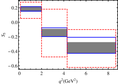
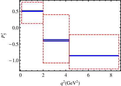
The choice of the two soft form factors defines a renormalisation scheme, and theory predictions made to a certain order in $\alpha_{s}$ or $\Lambda/m_{b}$ will exhibit a scheme dependence at the level of the neglected higher orders. This scheme dependence is illustrated in fig. 1 at order $\mathcal{O}(\alpha_{s})$ but at leading order in $\Lambda/m_{b}$ for the observable $S_{5}$ [22] and the optimised observable $P_{5}^{\prime}$ [4] in two different schemes (grey bands and blue(solid) boxes). The optimsed observables are constructed in such a way that any dependence on form factors drops out at LO in $\alpha_{s}$ and $\Lambda/m_{b}$. Therefore the uncertainty associated to the form factor input as well as the scheme dependence are pushed to order $\mathcal{O}(\alpha_{s})$ for the observable $P_{5}^{\prime}$ in contrast to the observable $S_{5}$. In addition we show the prediction which one would obtain using uncorrelated QCD form factors without resorting to large-recoil symmetries (red (dashed) boxes). The result demonstrates that in absence of a precise knowledge of correlations it is indispensable to make use of the soft form factor decomposition.

Figure 1: Scheme dependence in the prediction of the observables $S_{5}$ and $P_{5}^{\prime}$ at LO in $\Lambda/m_{b}$. Uncertainties are solely due to form factors. Grey bands correspond to the renormalisation scheme with LCSR input $\{V,A_{12}\}$ and blue (solid) boxes to the scheme with input $\{T_{1},A_{0}\}$. Red (dashed) boxes display results obtained using the full set of form factors without correlations. Form factor input is taken from ref. [16] in all cases.

2.2 Including power corrections

Since form factor uncertainties enter optimised observables only at order $\mathcal{O}(\alpha_{s},\Lambda/m_{b})$, $\Lambda/m_{b}$ corrections to large-recoil symmetry relations, called factorisable power corrections, are expected to be of the same order of magnitude. It is thus desirable to include them into the soft form factor decomposition. Even though there does not exist a direct calculation of these corrections, they can be assessed indirectly as they are contained in the LCSR results for the full form factors. Starting from a parametrisation

$$F^{\rm LCSR}(q^{2})=F^{\rm soft}(q^{2})+\Delta F^{\alpha_{s}}(q^{2})+a_{F}+b_{F}q^{2}+...$$ (3)

of the full LCSR form factors $F^{\rm LCSR}$, with $F^{\rm soft}$ representing the LO expression in the large-recoil limit and $\Delta F^{\alpha_{s}}$ the QCDF corrections, information on factorisable power corrections encoded in the parameters $a_{F},b_{F},...$ can be obtained from a fit to the full $F^{\rm LCSR}(q^{2})$.

This strategy has been proposed and followed for the first time in ref. [23]. The authors of ref. [23] fit the parameters $a_{F},b_{F}$ using central values for the form factors $F^{\rm LCSR},F^{\rm soft}$, and they interpret the result $\hat{a}_{F},\hat{b}_{F}$ as an order of magnitude estimate for the power corrections. In this spirit the uncertainties associated to power corrections are estimated by varying independently $-|\hat{a}_{F}|<a_{F}<|\hat{a}_{F}|$ and $-|\hat{b}_{F}|<b_{F}<|\hat{b}_{F}|$. In this approach, the central values of theory predictions are not affected by power corrections, in particular their scheme dependence is not reduced. Furthermore, the uncertainties associated with the power corrections are determined from the central values of the form factors, even though from the conceptual point of view they are related to the uncertainties of the latter. In particular in the hypothetical case in which the form factors are precisely known, i.e. their uncertainties (and the uncertainties of their power corrections) go to zero, the obtained error estimate for the power corrections would remain constant and different from zero. Finally, the method does not make use of the full information obtained from the fit as the definite and correlated signs of the fit parameters $\hat{a}_{F},\hat{b}_{F}$ get lost. In the light of the definite sign of the fit results, the symmetric variation of the $a_{F},b_{F},...$ around zero implies that power corrections are underestimated in one direction while they are overestimated in the other.

In our analysis we modify the approach of ref. [23] and go beyond it in several aspects. We keep the fit values $\hat{a}_{F},\hat{b}_{F},...$ as non-zero central values and vary

$$\hat{a}_{F}-\Delta\hat{a}_{F}<a_{F}<\hat{a}_{F}+\Delta\hat{a}_{F},...\;.$$ (4)

In order to fix the ranges $\Delta\hat{a}_{F},\Delta\hat{b}_{F},...$ for the variation, we consider an expanded version $F^{\rm LCSR}(q^{2})=A_{F}+B_{F}q^{2}/m_{B}^{2}+...$ of the full LCSR form factors and attribute to the power corrections an uncertainty of $10\%$ of the full form factor setting $\Delta\hat{a}_{F}=0.1A_{F},\Delta\hat{b}_{F}=0.1B_{F},...\;$. This procedure has the following features: The non-zero central values of the power corrections shift the central values of observables to the values which one would obtain using directly the full form factors. This implies that our predictions for the central values are scheme-independent. The error variation is performed with respect to the shifted central values implying a shift of the error bands with respect to the error bands obtained in ref. [23]. Our error estimate is conservative as it amounts to assigning an error of $\sim 100\%$ to the result from the fit, given the fact that the typical size of power corrections is $\Delta F^{\Lambda}\sim F\times\mathcal{O}(\Lambda/m_{b})\sim 0.1F$. Moreover, since the error ranges $\Delta\hat{a}_{F},\Delta\hat{b}_{B},...$ are introduced by hand, they can easily be adopted once information on the uncertainties of the LCSR form factors improves by smaller overall errors or better knowledge of correlations.

2.3 Correlations

Power corrections are constrained, on the one hand from exact kinematic relations to be fulfilled by the full form factors at $q^{2}=0$, and on the other hand by the choice of the renormalisation scheme for the soft form factors. These correlations, which have to be taken into account when the $a_{F},b_{F},...$ are varied within the ranges of eq. (4), are thus scheme-dependent. Taking for example $\{T_{1},A_{0}\}$ as soft form factors eliminates power corrections (and the corresponding uncertainties) in the form factors $T_{1}$ and $A_{0}$, while taking $\{V,A_{12}\}$ as input eliminates power corrections in $V$ and minimises their effects in $A_{1},A_{2}$. A change of the renormalisation scheme corresponds to the reshuffling of power corrections among the different form factors. An appropriate choice of the renormalisation scheme can therefore reduce the impact of power corrections on a certain observable by shifting the power corrections into those form factors to which the observable is less sensitive. In principle it is possible to choose for each observable the optimal scheme which minimises its individual error. Note, however, that in a global analysis one is forced to use the same scheme for all observables if one does not want to loose correlations among the observables.

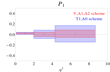
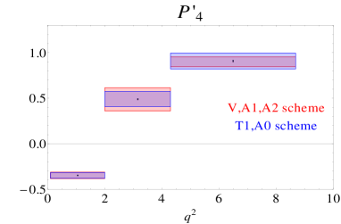
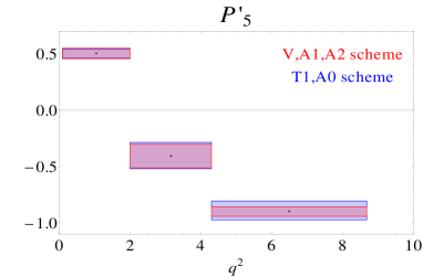
In fig. 2 we show our predictions including power corrections for the observables $P_{1}$, $P_{2}$, $P_{4}^{\prime}$ and $P_{5}^{\prime}$. We parametrised the power corrections as $a_{F}+b_{F}q^{2}/m_{B}^{2}+c_{F}q^{4}/m_{B}^{4}$ and we performed a flat scan of the $a_{F},b_{F},c_{F}$ over the sub-space allowed by the correlations. The blue bands represent the results obtained for the renormalisation scheme with $\{T_{1},A_{0}\}$ as input, while the red bands represent the results for the scheme with $\{V,A_{12}\}$. Since the observable $P_{5}^{\prime}$ showing the anomaly is much more sensitive to the vector form factor $V$ than to the tensor form factor $T_{1}$, and since the contribution of the form factor $A_{0}$ to observables is always suppressed by small lepton masses, the $\{V,A_{12}\}$-scheme is phenomenologically favoured compared to the $\{T_{1},A_{0}\}$-scheme.

Figure 2: Scheme dependence on the prediction of the observables $P_{1}$, $P_{2}$, $P_{4}^{\prime}$, $P_{5}^{\prime}$ in QCD factorisation. These results include factorisable power corrections as described in the text.

In ref. [13] we give detailed predictions in this scheme for all the $S_{i}$- and $P_{i}^{(\prime)}$-observables, including apart from the error associated to the factorisable power corrections also parametric errors, form factor errors and errors corresponding to non-factorisable power corrections. We note that for optimised observables and for input taken from ref. [16], parametric uncertainties, form factor uncertainties and uncertainties from factorisable power corrections are usually of the same order of magnitude, while uncertainties from non-factorisable power corrections are typically smaller. For ”non-optimised observables“, uncertainties are dominated by the form factor input as expected. For input taken from ref. [15], the uncertainties stemming from the form factors are generally smaller, in particular they are completely negligible for optimised observables.

3 Long-distance charm loop effects

The long-distance contribution from $c\bar{c}$ loops does not stand on the same footing as the factorisable power corrections discussed in the previous section. Its size is a debated issue, with some contributions considered in ref. [16] for $B\to K^{*}\mu^{+}\mu^{-}$ and further work (unfortunately only for $B\to K\mu^{+}\mu^{-}$) in ref. [24]. Very recently it has been claimed that low-scale non-perturbative and/or high-scale new physics contributions to the charm loop could explain the anomalous $B\to K^{*}\mu^{+}\mu^{-}$ data [25].

For an overall estimate of non-perturbative contributions from hadronic operators, we consider the terms $\Delta C_{9}$ in ref. [16], which include the LO perturbative contribution from $O_{1,2}$ together with non-factorisable soft-gluon emission from the charm loop. In order to separate the long-distance contribution $\delta C_{9}^{\rm LD}$, we subtract the perturbative contribution from $\Delta C_{9}$. We add this contribution to each amplitude $A_{i}^{L,R}$ ($i=\perp,\|,0$) by substituting

$$C_{9}\to C_{9}+s_{i}\delta C_{9}^{\rm{LD}}(q^{2})\ .$$ (5)

The result of the calculation in ref. [16] corresponds to setting $s_{i}=1$. However, since the computation of ref. [16] does not include all contributions, we prefer to interpret their result only as an order-of-magnitude estimate and to vary the parameters $s_{i}$ thus in the range $[-1,1]$. Through the independent variation of the $s_{i}$ we make sure that contributions to different amplitudes are not artificially correlated and we allow for the possibility of long-distance contributions with opposite signs in the different amplitudes.

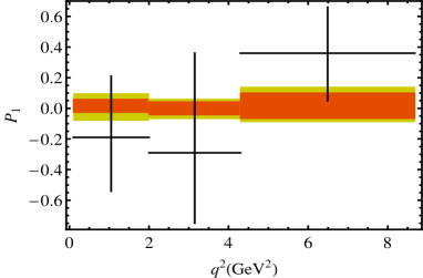
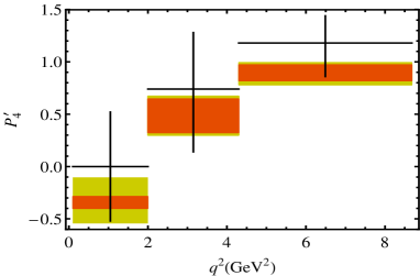
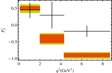
In fig. 3 we show our results where the long-distance $c\bar{c}$ correction is displayed as a separate band added in quadrature to the combined error from parametric uncertainties, form factors and power corrections. These plots constitute our predictions including charm-loop effects. We note that the discrepancy between theory and data in the third bin of $P_{5}^{\prime}$ remains also when QCD uncertainties from power corrections and from charm loops are included in the theory prediction. Results for all the $S_{i}$- and $P_{i}^{(\prime)}$-observables and further details can be found in ref. [13].

Figure 3: SM predictions for the observables $P_{1}$, $P_{2}$, $P_{4}^{\prime}$, $P_{5}^{\prime}$. The bands correspond to all uncertainties added in quadrature, not including (dark) and including (light) our estimate of long-distance charm-loop effects. The data points correspond to experimental data from LHCb [2, 3].

4 Conclusions

A QCDF-improved calculation based on soft form factors allows for precise predictions of $B\to K^{*}\mu^{+}\mu^{-}$ observables even in the absence of knowledge on correlations of the form factor uncertainties.

In optimised observables large-recoil symmetries enforce a cancellation of the form factors at LO in $\alpha_{s}$ and $\Lambda/m_{b}$ and hence such observables exhibit a reduced sensitivity to form factor uncertainties. They are thus sensitive to subleading power corrections of order $\Lambda/m_{b}$ for which this suppression mechanism breaks down as they break the large-recoil symmtries. We have presented a systematic approach to include factorisable power corrections into a calculation based on soft form factors. We have further demonstrated that the impact of factorisable power corrections can be reduced, i.e. the precision of the predictions of observables can be increased, by a suitable choice of the renormalisation scheme for the soft form factors.

Finally we have discussed long-distance effects from charm loops based on the partial calculation of ref. [16] whose results we use as an estimator for the expected order of magnitude.

Our complete results for two different sets of LCSR form factors [15, 16] can be found in ref. [13].

References

- [1] S. Descotes-Genon, T. Hurth, J. Matias and J. Virto, JHEP 1305 (2013) 137 [arXiv:1303.5794 [hep-ph]].
- [2] R. Aaij et al. [LHCb Collaboration], JHEP 1308, 131 (2013) [arXiv:1304.6325, arXiv:1304.6325 [hep-ex]].
- [3] R. Aaij et al. [LHCb Collaboration], Phys. Rev. Lett. 111 (2013) 191801 [arXiv:1308.1707 [hep-ex]].
- [4] S. Descotes-Genon, J. Matias, M. Ramon and J. Virto, JHEP 1301 (2013) 048 [arXiv:1207.2753 [hep-ph]].
- [5] D. Becirevic and E. Schneider, Nucl. Phys. B 854, 321 (2012) [arXiv:1106.3283 [hep-ph]].
- [6] J. Matias, F. Mescia, M. Ramon and J. Virto, JHEP 1204 (2012) 104 [arXiv:1202.4266 [hep-ph]].
- [7] J. Matias and N. Serra, arXiv:1402.6855 [hep-ph].
- [8] S. Descotes-Genon, J. Matias and J. Virto, Phys. Rev. D 88 (2013) 074002 [arXiv:1307.5683 [hep-ph]].
- [9] W. Altmannshofer and D. M. Straub, Eur. Phys. J. C 73 (2013) 2646 [arXiv:1308.1501 [hep-ph]]; see also the talk by W. Altmannshofer at “CKM 2014”.
- [10] F. Beaujean, C. Bobeth and D. van Dyk, arXiv:1310.2478 [hep-ph].
- [11] R. R. Horgan, Z. Liu, S. Meinel and M. Wingate, arXiv:1310.3887 [hep-ph].
- [12] T. Hurth, F. Mahmoudi and S. Neshatpour, arXiv:1410.4545 [hep-ph].
- [13] S. Descotes-Genon, L. Hofer, J. Matias and J. Virto, arXiv:1407.8526 [hep-ph].
- [14] M. Beneke and T. Feldmann, Nucl. Phys. B 592 (2001) 3 [hep-ph/0008255].
- [15] P. Ball and R. Zwicky, Phys. Rev. D 71 (2005) 014015 [hep-ph/0406232].
- [16] A. Khodjamirian, T. Mannel, A. A. Pivovarov and Y. -M. Wang, JHEP 1009 (2010) 089 [arXiv:1006.4945 [hep-ph]].
- [17] V. Braun, Talk at “Lattice meets continuum” 2014.
- [18] J. Charles, A. Le Yaouanc, L. Oliver, O. Pene and J. C. Raynal, Phys. Rev. D 60, 014001 (1999) [hep-ph/9812358].
- [19] C. W. Bauer, S. Fleming, D. Pirjol and I. W. Stewart, Phys. Rev. D 63, 114020 (2001) [hep-ph/0011336].
- [20] M. Beneke, T. Feldmann and D. Seidel, Nucl. Phys. B 612 (2001) 25 [hep-ph/0106067].
- [21] B. Grinstein and D. Pirjol, Phys. Rev. D 70 (2004) 114005 [hep-ph/0404250].
- [22] W. Altmannshofer, P. Ball, A. Bharucha, A. J. Buras, D. M. Straub and M. Wick, JHEP 0901 (2009) 019 [arXiv:0811.1214 [hep-ph]].
- [23] S. Jäger and J. Martin Camalich, JHEP 1305 (2013) 043 [arXiv:1212.2263 [hep-ph]].
- [24] A. Khodjamirian, T. Mannel and Y. M. Wang, JHEP 1302 (2013) 010 [arXiv:1211.0234 [hep-ph]].
- [25] J. Lyon and R. Zwicky, arXiv:1406.0566 [hep-ph].