Algorithms for Mapping Parallel Processes onto
Grid and Torus Architectures

Abstract

Static mapping is the assignment of parallel processes to the processing elements (PEs) of a parallel system, where the assignment does not change during the application’s lifetime. In our scenario we model an application’s computations and their dependencies by an application graph. This graph is first partitioned into (nearly) equally sized blocks. These blocks need to communicate at block boundaries. To assign the processes to PEs, our goal is to compute a communication-efficient bijective mapping between the blocks and the PEs.

This approach of partitioning followed by bijective mapping has many degrees of freedom. Thus, users and developers of parallel applications need to know more about which choices work for which application graphs and which parallel architectures. To this end, we not only develop new mapping algorithms (derived from known greedy methods). We also perform extensive experiments involving different classes of application graphs (meshes and complex networks), architectures of parallel computers (grids and tori), as well as different partitioners and mapping algorithms. Surprisingly, the quality of the partitions, unless very poor, has little influence on the quality of the mapping.

More importantly, one of our new mapping algorithms always yields the best results in terms of the quality measure maximum congestion when the application graphs are complex networks. In case of meshes as application graphs, this mapping algorithm always leads in terms of maximum congestion and maximum dilation, another common quality measure.

1 Introduction

Symmetric dependencies of computations within a parallel application can be modeled by an undirected graph $G_{a}$, called application graph, e. g. the mesh of a numerical simulation. Iterative algorithms in such a simulation act upon the vertices of $G_{a}$, and for each such vertex require the values of the neighboring vertices from the previous iteration. Thus, a vertex of $G_{a}$ represents some computation, and an edge of $G_{a}$ indicates a dependency between computations, i. e. an exchange of data. It is important to note that this modeling is not restricted to simulations at all. In fact, the nodes of $G_{a}$ could represent arbitrary parallel processes and the edges symmetric communication requirements between the processes.

Typically, running an application on computers with distributed parallelism requires the application graph to be spread over the computer’s processing elements. One way to carry out this task, called static mapping, is to (i) partition the application graph $G_{a}$ into blocks of equal size (or of equal weight in case the computational requirements at the nodes are not homogeneous) for load balancing purposes and (ii) map the blocks of $G_{a}$ onto the processing elements (PEs) of a parallel computer, see Figure 1. Mapping may involve the communication graph $G_{c}$, whose vertices represent the blocks of $G_{a}$’s partition and whose edges indicate block neighborhood and therefore communication between different PEs.

The parallel computer is often represented as a graph $G_{p}$, called processor graph (or topology graph), the vertices of which represent the PEs, and the edges of which represent physical communication links between the PEs. We require that $G_{c}$ has the same number of vertices as $G_{p}$ and make the assumption that $G_{p}$ is sparse, which is true for many real architectures today [1]. In this paper we address the problem of finding a bijective mapping $\Pi$ of $G_{c}$’s vertex set onto $G_{p}$’s vertex set (processors) that is communication-efficient. We refer to $\Pi$ as bijective topology mapping or simply mapping. One can also see the problem as embedding the guest graph $G_{c}$ into the host graph $G_{p}$.

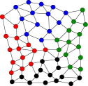
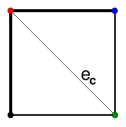
(a) (b) (c)

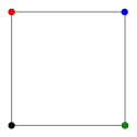
Figure 1: (a) Application graph $G_{a}$ with $4$-way partition indicated by colors. (b) Communication graph $G_{c}$ induced by $G_{a}$ and the partition. $G_{c}$ expresses the neighborhood relations of $G_{a}$’s blocks. Edge weights (shown through width) indicate communication volumes between blocks. (c) Processor graph $G_{p}$. Nodes and edges represent the PEs and the communication links, respectively. Communication between the green and the red block in $G_{c}$, i. e. via $e_{c}$, requires two hops in $G_{p}$.

Motivation. Communication costs are crucial for the scalability of many parallel applications. Static mapping, in turn, is crucial when it comes to keeping communication costs under control through (i) providing a partitioning with few edges between blocks and (ii) mapping nearby blocks onto nearby PEs: due to the sparse nature of many large-scale parallel computers, communication costs may vary by several orders of magnitude depending on the distance between the PEs involved [2]. Also, numerous recent applications involve massive complex networks such as social networks or web graphs [3]. These networks usually lead to denser communication graphs and make improved mapping strategies even more desirable.

Contribution. We investigate numerous algorithms for static mapping, the scenario being that an application graph is first partitioned into blocks, followed by a bijective mapping of the blocks onto the nodes of a processor graph. The graph partitioners we employ are the state-of-the-art packages METIS [4] and KaHIP [5]. While METIS is widely used for graph partitioning and has been employed for mapping before, it is the first time that the high-quality partitioner KaHIP is used in the mapping context.

To assess and improve the performance of mapping algorithms, we implement several state-of-the-art methods. Moreover and more importantly, we develop and implement two new algorithms as straightforward, yet very effective adaptations of existing greedy algorithms.

The three most striking results of our extensive mapping experiments on meshes and complex networks as application graphs, as well as grids and tori as processor graphs, are: First, the strengths and weaknesses of the mapping algorithms are, to a large extent, independent of the class of application graphs (mesh or complex network) and the processor graphs. Second, the graph partitioner and its partitioning quality is of minor importance for the quality of the mapping. Third, for complex networks as application graphs, one of our new mapping algorithms always yields the best quality in terms maximum congestion. In case of meshes, this mapping algorithm always leads in terms of maximum congestion and maximum dilation.

2 Preliminaries

2.1 Problem Description

We represent the communication of a parallel application as a graph $G_{c}=(V_{c},E_{c},\omega_{c})$, where a weight $\omega_{c}(\{u,v\})$, $\{u,v\}\in E_{c}$, indicates the volume of communication between $u$ and $v$, i. e. between the corresponding blocks of the application graph.

The parallel computer takes the form of a graph $G_{p}=(V_{p},E_{p},\omega_{p})$, the processor graph. Here, $\omega_{p}~{}:~{}E_{p}\mapsto\mbox{\rm I$\!$N}$ indicates the bandwidths of the physical communication links. We require $|V_{p}|=|V_{c}|$.

Our aim is to find a bijective topology mapping (short mapping) $\Pi:V_{c}\mapsto V_{p}$ that minimizes the overhead due to communication between the processes. A first graph-theoretic definition of the overhead (costs) was given in [6]. In the following we present three aspects of overhead (for more in-depth definitions see [7]).

An edge $e_{c}=\{u_{c},v_{c}\}$ of $G_{c}$ gives rise to communication between $\Pi(u_{c})$ and $\Pi(v_{c})$ on $G_{p}$. Sending a unit of information along a path $P$ in $G_{p}$ with edges $e_{1},\dots e_{l}$ takes time at least $t(P)=\sum_{i=1}^{l}(1/\omega_{p}(e_{i}))$. Sending all information via an edge $e_{c}=\{u_{c},v_{c}\}\in E_{c}$, i. e. from processes in $u_{c}$ to processes in $v_{c}$, then takes time at least

$$d(e_{c}) =d(e_{c},\Pi)=\omega_{c}(u_{c},v_{c})~{}t(\Pi(u_{c}),\Pi(v_{c})),\mbox{ where}$$

$$t(u_{p},v_{p}) =\min(t(P)~{}|~{}\mbox{$P$ connects $u_{p}$ and $v_{p}$})$$ (1)

Thus, maximum and average dilation, defined as

$$mD(\Pi) =\max_{e_{c}\in E_{c}}d(e_{c})\mbox{~{}and}$$ (2)

$$aD(\Pi) =(\sum_{e_{c}\in E_{c}}d(e_{c}))/|E_{c}|\mbox{~{},}$$ (3)

respectively, provide lower bounds for the communication time of a parallel application, $mD(\Pi)$ being the tighter lower bound.

When multiple messages are exchanged at the same time, more than one of them may be routed via the same edge. Hence, if $c(e)$ denotes the total volume of communication routed via $e\in E_{p}$, divided by the bandwidth $\omega(e)$, then the maximum (weighted) congestion

$$mC(\Pi):=max_{e_{c}\in E_{c}}c(e_{c})$$ (4)

provides another lower bound for the time. Minimizing $mD(\Pi)$, $aD(\Pi)$ and $mC(\Pi)$ is NP-hard, cf. Garey and Johnson [8] and more recent work [7, 9]. Due to the problem’s complexity, exact mapping methods are only practical in special cases. Leighton’s book [10] discusses embeddings between arrays, trees, and hypercubes.

As in previous studies [7], we assume that the routing algorithm sends the messages on uniformly distributed shortest paths in $G_{p}$. In particular, the routing algorithm is oblivious to the utilization of the parallel system.

2.2 Graph partitioning

Given a graph $G=(V,E)$ and a number of blocks $k>0$, the graph partitioning problem asks for a division of $V$ into $k$ pairwise disjoint subsets $V_{1},\dots,V_{k}$ (blocks) such that no block is larger than $(1+\varepsilon)\cdot\left\lceil\frac{|V|}{k}\right\rceil,$ where $\varepsilon\geq 0$ is the allowed imbalance. The most widely used objective function is the edge cut (whose minimization is $\mathcal{NP}$-hard [8]), i. e., the total weight of the edges between different blocks. Yet, a more important factor for modeling the communication cost of parallel iterative graph algorithms seems to be the maximum communication volume (MCV) [11], which has received growing attention recently, e. g. in the 10th DIMACS Implementation Challenge on graph partitioning. MCV considers the worst communication volume taken over all blocks $V_{p}$ ($1\leq p\leq k$) and thus penalizes imbalanced communication: $MCV(V_{1},\dots,V_{k}):=\max_{p}\sum_{v\in V_{p}}|\{V_{i}~{}|~{}\exists\{u,v\}\in E\mbox{ with }u\in V_{i}\neq V_{p}\}|.$

3 Related Work

In this section we give a brief overview of algorithms for static mapping. More on topology mapping can be found in [12, 13] and particularly in Pellegrini’s survey [14].

It should be mentioned that partitioning and mapping can be done simultaneously, i. e. communication between PEs is taken into account already during partitioning [15, 16, 17]. In this paper, however, we focus on the complementary approach where partitioning and topology mapping form different stages of a software pipeline.

One can apply a wide range of optimization techniques to the topology mapping problem. Hoefler and Snir [7] employ (among others) the Reverse Cuthill-McKee (RCM) algorithm, originally devised for minimizing the bandwidth of a sparse matrix [18]. If both $G_{c}$ and $G_{p}$ are sparse, the simultaneous optimization of both graph layouts can lead to good mapping results [19].

A common approach to static mapping, i. e., partitioning and topology mapping combined, is to recursively partition $G_{a}$ and $G_{p}$ in the same fashion, i. e. such that the number of blocks and sub-blocks per block is equal on each level [20]. Such a hierarchical approach to mapping may take into account the actual hierarchy of a heterogeneous multi-core cluster [21]. Typically, the number of sub-blocks per block is small. Thus, on the scope of an individual block, an optimal mapping of a block’s sub-blocks can be found by evaluating all possibilities. If the number of sub-blocks is two, the method is called dual recursive bisection. It has been shown effective in the software Scotch [19]. While an optimal mapping of a block’s sub-blocks on the scope of an individual block is not an issue in dual recursive bisection, neighboring relations between sub-blocks of different blocks still pose a challenge. In this paper we apply dual recursive bisection to the pair $(G_{c},G_{p})$ instead of $(G_{a},G_{p})$. This (basic) form of dual recursive bisection does not take into account neighboring relations between the sub-blocks of different blocks (as in [7]).

Greedy approaches such as the ones by Hoefler and Snir [7] and Brandfass et al. [22] build on the idea of increasing a mapping by successively adding new maps $v_{c}\rightarrow v_{p}$ such that (i) $v_{c}$ has maximal communication volume with one or all of the already mapped vertices of $G_{c}$ and (ii) $v_{p}$ has minimal distance to one or all of the already mapped vertices of $G_{p}$. For more details see Sections 4.1.

Hoefler and Snir [7] compare RCM, DRB and a greedy approach experimentally on abstractions of three real architectures. While their results do not show a clear winner, they confirm previous studies [14] in that performing mapping at all is worthwhile. It is important to note, however, that Hoefler and Snir perform mapping from reordered matrices, not from partitioned graphs as we do here.

Many metaheuristics have been used to solve the mapping problem. Uçar et al. [23] implement a large variety of methods within a clustering approach, among them genetic algorithms, simulated annealing, tabu search, and particle swarm optimization. The authors require, however, that the processor graph is homogeneous, i. e. $t(u_{p},v_{p})$ depends only on whether $u_{p}=v_{p}$ or not. Our approach is more general than theirs in that we allow $t(u_{p},v_{p})$ to take different values for $u_{p}\not=v_{p}$ (see Equation 2.1).

Bhatele et al. [24] discuss topology-aware mappings of different MPI communication patterns on emerging architectures. Better mappings avoid communication hot spots and reduce communication times significantly. Geometric information can also be helpful for finding good mappings on regular architectures such as tori [25].

4 Methods for Topology Mapping

The simplest topology mapping is the identity, i. e. when block $i$ of the application graph (or vertex $i$ of the communication graph $G_{c}$) is mapped onto node $i$ of the processor graph $G_{p}$, $1\leq i\leq k$. We refer to this mapping as Initial. It depends on how the graph partitioner, in our case METIS or KaHIP, numbers the blocks and on how the nodes of $G_{p}$ are numbered. In our experiments $G_{p}$ is a 2D or 3D grid or torus since such topologies are used in real architectures, e. g. tori for BlueGene [26]. The nodes are ordered lexicographically w. r. t. the nodes’ canonical integer coordinates. We also carry along a mapping called Random, where the bijection $\Pi:\{1,\dots,k\}\mapsto\{1,\dots,k\}$ is random. The latter is done for comparison purposes, keeping in mind that Random is usually a very bad solution.

Four algorithms in our collection, i. e., RCM, DRB, GreedyAll and GreedyMin are from the literature (for RCM and DRB see Section 1 and [18, 7]). Algorithms GreedyAll and GreedyMin are described in Section 4.1 (also see the references therein). There we also specify the last two algorithms, GreedyAllC and GreedyMinC, which are variants of GreedyAll and GreedyMin and which, to our knowledge, are new.

4.1 Greedy Algorithms

As a prerequisite for the algorithms described in this section we need to compute $t(\cdot,\cdot)$ once for a given processor graph $G_{p}$ (see Equation 2.1). Using Johnson’s algorithm [27, 28] we can do so in time $\mathcal{O}(|V_{p}|^{2}\log|V_{p}|$ $+$ $|V_{p}||E_{p}|)$. Since $G_{p}$ is sparse, this amounts to $\mathcal{O}(|V_{p}|^{2}\log|V_{p}|)=\mathcal{O}(|V_{c}|^{2}\log|V_{c}|)$. This running time is not included in the running times for the greedy algorithms in this section, as $t(\cdot,\cdot)$ is computed only once for a given processor graph.

The mapping algorithm GreedyAll consists of the “construction method” proposed in [22]. Using our terminology, the algorithm starts by picking a node $v^{0}_{c}$ of $G_{c}$ such that $\sum_{e=\{v^{0}_{c},v_{c}\}\in E_{c}}\omega(e)$ is maximal, i. e. $v^{0}_{c}$ is a vertex whose communication with neighboring vertices is heaviest. Then, it computes for each vertex $v_{p}$ of $G_{p}$ the term $\sum_{u_{p}\in V_{p}}t(u_{p},v_{p})$. Here, $t(u_{p},v_{p})$ is the (minimum) time needed to send a unit of information from $u_{p}$ to $v_{p}$ (see Section 2.1). A vertex $v^{0}_{p}$ for which this sum is minimal (a most central node in $G_{p}$ w. r. t. communication time) then becomes the vertex onto which $v^{0}_{c}$ is mapped. The experiments of this paper involve processor graphs which are grids and tori. On the latter all nodes are equally central.

The remaining pairs $(v^{i}_{c},v^{i}_{p})$, $i\geq 1$, are formed as follows. First, a not yet mapped vertex $v^{i}_{c}$ of $G_{c}$ is found such that $\sum^{i-1}_{j=0}\omega_{c}(\{v^{j}_{c},v^{i}_{c}\})$ is maximal, i. e. $v^{i}_{c}$ is a vertex that communicates most heavily with the already mapped vertices. Then, a not yet mapped vertex $v^{i}_{p}$ of $G_{p}$ is found such that $\sum^{i-1}_{j=0}t(v^{j}_{p},v^{i}_{p})$ is minimal, i. e. a vertex that is most central w. r. t. the already mapped vertices of $G_{p}$. Note that the choices of $v^{i}_{c}$ and $v^{i}_{p}$ are independent of each other. Our implementation of GreedyAll has running time $\mathcal{O}(|V_{c}|^{2})$. This running time is achieved by updating vectors $sum_{c}$ ($sum_{p}$) that, for each vertex $v_{c}$ ($v_{p}$) which has not been mapped yet, stores the sum of the edge weights (distances) to the vertices in $G_{c}$ ($G_{p}$) that have been mapped already. We use the same two vectors in GreedyAllC, see Algorithm 1.

The mapping algorithm GreedyMin stems from [7]. Its general idea is the same as that behind GreedyAll. The only differences are that (i) $v^{0}_{p}$ is picked randomly, (ii) $v^{i}_{c}$ ($i\geq 1$) is chosen such that $max^{i-1}_{j=0}\omega_{c}(\{v^{i}_{c},v^{j}_{c}\})$ is maximal, and (iii) $v^{i}_{p}$ ($i\geq 1$) is chosen such that $t(v^{i-1}_{p},v^{i}_{p})$ is minimal. Again, as in GreedyAll, the choices of $v^{i}_{c}$ and $v^{i}_{p}$ are independent of each other. Our implementation of GreedyMin (which is less generic than that in [7]) has running time $\mathcal{O}(|V_{c}|^{2})$.

4.2 GreedyAllC and GreedyMinC

Neither GreedyAll nor GreedyMin link the choices of $v^{c}_{i}$ and $v^{p}_{i}$. Both algorithms aim at (i) a high communication volume of $v^{c}_{i}$ with all or one of the already mapped vertices of $G_{c}$ and (ii) a high centrality of $v^{p}_{i}$ w. r. t. all or one of the already mapped vertices of $G_{p}$. The actual increase of communication times caused by the new pair $(v^{c}_{i},v^{p}_{i})$ (increase w. r. t. the partial mapping defined so far) is not considered.

We therefore propose new variants GreedyAllC and GreedyMinC. They take this increase of communication time into account. Specifically, the choice of $v^{i}_{p}$ depends on the choice of $v^{i}_{c}$ (same as in $\textsc{GreedyAll}/\textsc{GreedyMin}$). Let $v_{p}$ be a candidate for being mapped onto by $v^{i}_{c}$. Then, (minimal) times of communication between $v^{i}_{c}$ and the vertices of $G_{c}$ that have been mapped before, i. e. $v^{0}_{c},\dots v^{i-1}_{c}$, amount to

$$\sum(\omega_{c}(\{v^{i}_{c},v_{c}\}~{}t(v_{p},\Pi(v_{c})))~{}\mid~{}\{v^{i}_{c},v_{c}\}\in E_{c}~{},v_{c}\in\{v^{0}_{c},\dots v^{i-1}_{c}\})$$ (5)

Analogous to GreedyAllC and GreedyMinC, we set $v^{i}_{p}$ to some $v_{p}$ such that the expression in Equation 5 is minimal. Thus, our objective function for choosing $v_{p}$, i. e. Equation 5, is about actual communication times and not just distances on $G_{p}$. We have experimented with replacing the sum in Equation 5 by the maximum and found out that this tends to decrease the quality of the mappings. For the pseudocode of GreedyAllC see Algorithm 1.

Algorithm 1 The algorithm GreedyAllC.
Input: Communication graph $G_{c}=(V_{c},E_{c},\omega_{c})$ and processor graph $G_{p}=(V_{p},E_{p},\omega_{p})$ with $|V_{c}|=|V_{p}|$.
Output: Pairs $(v^{i}_{c},v^{i}_{p})$, $0\leq i<|V_{c}|$, such that $\Pi~{}:~{}V_{c}\mapsto V_{p}$ defined by $\Pi(v^{i}_{c})=v^{i}_{p}$ is a bijective mapping with low values of $mC(\Pi)$, $mD(\Pi)$ and $aD(\Pi)$.

1:Find $v^{0}_{c}\in V_{c}$ with maximal $\sum_{e=\{v^{0}_{c},v_{c}\}\in E_{c}}\omega(e)$

2:Find $v^{0}_{p}\in V_{p}$ with minimal $\sum_{u_{p}\in V_{p}}t(u_{p},v_{p})$

3:Create vectors $sum_{c}$ and $sum_{p}$ of length $|V_{c}|$

4:Initialize entries of $sum_{c}$ to zero and entries of $sum_{p}$ to one

5:for $i\leftarrow 0,\dots,|V_{c}|-2$ do

6:     $sum_{c}(v^{i}_{c})\leftarrow-1$ /* Mark $v^{i}_{c}$ as assigned */

7:     $sum_{p}(v^{i}_{p})\leftarrow\textsc{int\_max}$ /* Mark $v^{i}_{p}$ as assigned */

8:     for all $e_{c}=\{v^{i}_{c},w\}\in E_{c}$ do

9:         if $sum_{c}[w]\geq 0$ then /* $w$ is not yet assigned */

10:              $sum_{c}[w]\leftarrow sum_{c}[w]+\omega_{c}(e_{c})$

11:         end if

12:     end for

13:     Pick $v^{i+1}_{c}$ such that $sum_{c}(v^{i+1}_{c})$ is maximal

14:     for $j\leftarrow 1,\dots,|V_{p}|-1$ do

15:         if $sum_{p}[j]<\textsc{int\_max}$ then

16:              /* $j$ is not yet assigned */

17:              $sum_{p}[j]\leftarrow 0$

18:              for all $e_{c}=\{v^{i+1}_{c},w\}\in E_{c}$ do

19:                  if $sum_{c}[w]<0$ then

20:                       /* $w$ has already been assigned, i. e. $\Pi(w)$ is defined */

21:                       $sum_{p}[j]\leftarrow sum_{p}[j]+\omega_{c}(e_{c})*t(j,\Pi(w))$

22:                  end if

23:              end for

24:         end if

25:     end for

26:     Pick $v^{i+1}_{p}$ such that $sum_{p}(v^{i+1}_{p})$ is maximal

27:end for

Proposition 1

The running time of GreedyAllC is $\mathcal{O}(|V_{c}||E_{c}|)$.

Proof

The outermost loop from line 5 to line 27 and the inner loop from line 8 to line 12 take amortized time $\mathcal{O}(|E_{c}|)$. So does the outer loop from line 14 to line 25 and the inner loop from line 18 to line 23. Since the latter two loops are contained in the outermost loop from line 5 to line 27, the running time of Algorithm 1 is indeed $\mathcal{O}(|V_{c}||E_{c}|)$. Even a trivial implementation of lines 13 and 26 (with running time $\mathcal{O}(|V_{c}|)$) does not change the result.

The running time for GreedyMin is the same as for GreedyAllC because the two algorithms differ only at lines 1 to 4, and the running times of both algorithms are not determined by this part.

5 Experiments

In this section we specify our test instances, our experimental setup and the way we evaluate the mapping algorithms.

Test Instances.

The application graphs fall into two classes: The class WalshawLarge consists of the eight largest graphs in Walshaw’s graph partitioning archive [29], and the class ComplexNets consists of 12 complex networks (see Tables 1 and 2). The latter form a subset of the 15 complex networks used in [30] for partitioning experiments. It turned out, however, that KaHIP [gpMetis with $k$-way partitioning, respectively], while respecting the allowed imbalance, occasionally generated empty blocks for the complex network p2p-Gnutella [as-22july06 and loc-gowalla_edges]. Using gpMetis with recursive bisection instead of k-way partitioning was not an option because gpMetis then quite often violated the balance constraint and produced blocks heavier than $(1+\epsilon)$ times the average block size (only on complex networks). For each of the classes WalshawLarge and ComplexNets the benchmarking comprises the following processor graphs.

• 2DGrid($16\times 16$), 2DGrid($32\times 32$), 3DGrid($8\times 8\times 8$)

• 2DTorus($16\times 16$), 2DTorus($32\times 32$), 3DTorus($8\times 8\times 8$)

Table 1: Meshes used for benchmarking

Name	#vertices	#edges
fe_tooth	78 136	452 591
fe_rotor	99 617	662 431
598a	110 971	741 934
fe_ocean	143 437	409 593
144	144 649	1 074 391
wave	156 317	1 059 331
m14b	214 765	1 679 018
auto	448 695	3 314 611

Table 2: Complex networks used for benchmarking.

Name	#vertices	#edges	Type
PGPgiantcompo	10 680	24 316	largest connected component in network of PGP users
email-EuAll	16 805	60 260	network of connections via email
soc-Slashdot0902	28 550	379 445	news network
loc-brightkite_edges	56 739	212 945	location-based friendship network
coAuthorsCiteseer	227 320	814 134	citation network
wiki-Talk	232 314	1 458 806	network of user interactions through edits
citationCiteseer	268 495	1 156 647	citation network
coAuthorsDBLP	299 067	977 676	citation network
web-Google	356 648	2 093 324	hyperlink network of web pages
coPapersCiteseer	434 102	16 036 720	citation network
coPapersDBLP	540 486	15 245 729	citation network
as-skitter	554 930	5 797 663	network of internet service providers

Experimental Setup.

All computations are sequential and done on a workstation with two 4-core Intel(R) Core(TM) i7-2600K processors at 3.40GHz. Our code is written in C++ and compiled with GCC 4.7.1.

Evaluation.

The benchmarking of the mapping algorithms described in Section 4 is done separately on the classes WalshawLarge and ComplexNets. First, graphs from both classes are partitioned into 256, 512 and 1024 parts using the graph partitioner KaHIP v. 0.62 (http://algo2.iti.kit.edu/documents/kahip/) [31]. In particular, the meshes and social networks are partitioned with the configuration eco and ecosocial, respectively. The allowed imbalance is always $1.03$, i. e. $\epsilon=3\%$. To recursively bipartition $G_{c}$ and $G_{p}$ during DRB, we also use KaHIP (configurations fast and ecofast, perfect balance).

Since the partitioning process depends on random choices, we run KaHIP with 20 different seeds. For each seed we construct a communication graph $G_{c}$ from the partition, map $G_{c}$ onto all processor graphs with the same number of vertices and then compute the minimum, the arithmetic mean and the maximum of the mapping’s runtime $t$, $mC$ (see Equation 4), $mD$ and $aD$ (see Equation 2). Thus we arrive at the values $t_{min}$, $t_{mean}$, $t_{max}$, $mC_{min}$, etc. (twelve values for each combination of $G_{c}$, $G_{p}$, and a mapping algorithm).

Next we form the geometric means of the twelve values over all graphs in WalshawLarge and ComplexNets, respectively. Thus we arrive at twelve values $t^{gm}_{min}$, $\dots$ for any combination of a graph class (WalshawLarge or ComplexNets), a processor graph, and a mapping algorithm. Finally, the last 9 values (all except runtimes) are set into proportion to the corresponding values for Initial. This yields the values $QmC^{gm}_{min}$, $QmC^{gm}_{mean}$, $QmC^{gm}_{max}$, $QmD^{gm}_{min}$, $QmD^{gm}_{mean}$, $QmD^{gm}_{max}$, $QaD^{gm}_{min}$, $QaD^{gm}_{mean}$ and $QaD^{gm}_{max}$. A $Q$-value smaller than one means that the quality is higher than that of Initial because we are minimizing.

We also investigate the influence of graph partitioning on the quality of the mapping algorithms. In addition to using KaHIP as described above, we apply two variants of METIS v. 5.1.0 [4]

1. We run gpMetis with the option of $k$-way partitioning, an allowed imbalance of $1.03$ and $20$ seeds (imbalance and seed number are as for KaHIP).

2. We run ndMetis with $20$ seeds. This results in a fill-reducing ordering of $G_{a}$’s adjacency matrix. The ordering is then turned into a partitioning of $G_{a}$ by going through the vertices in the new order and assigning block numbers such that all blocks have almost equal size (maximal deviation is one vertex). We are aware that using ndMetis in this way is not a good choice in view of partitioning quality (ndMetis is made for other purposes). We proceed like this, however, because we wish to test our collection of mapping algorithms on partitions with mediocre edge cut and MCV.

We indicate the METIS-based graph partitioning that is underlying a mapping algorithm by using the subscripts g and n when employing gpMetis and ndMetis, respectively. As an example, $\textsc{greedyAllC}_{\textsc{n}}$ means that we applied GreedyAllC to partitions obtained via ndMetis.

Finally, for each $x\in\{t^{gm}_{min},\dots\,QaD^{gm}_{max}\}$ (this set has 12 values), we form quotients $\mathcal{Q}x$ of the form

$$\frac{\mbox{$x$ from {KaHIP} partitions}}{\mbox{$x$ from {gpMetis} partitions}}\mbox{~{},~{}}\frac{\mbox{$x$ from {KaHIP} partitions}}{\mbox{$x$ from {ndMetis} partitions}}$$

As an example, $\mathcal{Q}aD^{gm}_{max}=3.2098$ for $\textsc{greedyAllC}_{\textsc{n}}$ in Table 5 means that $aD^{gm}_{max}$ is worse by a factor of $3.2098$ if ndMetis is used instead of KaHIP for mapping meshes onto 2DGrid($16\times 16$).

6 Results

6.1 Mapping of Meshes onto Grids and Tori

Table 3: Performance of gpMetis and ndMetis on meshes compared to KaHIP. Values smaller than one indicate that $\textsc{gpMetis}/\textsc{ndMetis}$ is faster or that the quality the $\textsc{gpMetis}/\textsc{ndMetis}$-partitions is higher.

	$Time^{gm}_{min}$	$Time^{gm}_{mean}$	$Time^{gm}_{max}$	$Cut^{gm}_{min}$	$Cut^{gm}_{mean}$	$Cut^{gm}_{max}$	$MCV^{gm}_{min}$	$MCV^{gm}_{mean}$	$MCV^{gm}_{max}$
gpMetis	0.0462	0.0451	0.0440	1.0101	1.0101	1.0121	0.9970	1.0449	1.1601
ndMetis	0.1026	0.0999	0.0985	2.2075	2.2371	2.2472	6.0976	5.9880	5.7471

Table 3 shows a comparison of KaHIP partitions with partitions from gpMetis and ndMetis. We measure running time, edge cut and MCV. As above, we record the best, mean and worst result over $20$ seeds and calculate the geometric means of these numbers over all meshes in our collection — giving rise to the numbers $Time^{gm}_{max},\dots,MCV^{gm}_{max}$ in Table 3. In terms of partition quality, gpMetis performs significantly poorer than KaHIP only in terms of $MCV^{gm}_{mean}$ and $MCV^{gm}_{max}$. Here gpMetis is worse by $4.49\%$ and $16.01\%$, respectively. The partitions that we derived from ndMetis (in a deliberately sub-optimal way) fall back drastically both in terms of the edge cut and MCV. In particular, $Cut^{gm}_{mean}=2.2371$ and $MCV^{gm}_{mean}=5.988$, which means that the edge cut from ndMetis is more than double and that MCV increases almost six times if ndMetis is used instead of KaHIP.

Table 4 shows the quality of the mapping algorithms for (i) partitions based on KaHIP and (ii) mapping onto the $16\times 16$ torus. Tables I - V in the Appendix support the following results.

Table 4: Mapping of meshes onto 2DTorus($16\times 16$). Times $t^{gm}_{min}$, $t^{gm}_{mean}$ and $t^{gm}_{max}$ are in milliseconds.

Algo	$t^{gm}_{min}$	$t^{gm}_{mean}$	$t^{gm}_{max}$	$QmC^{gm}_{min}$	$QmC^{gm}_{mean}$	$QmC^{gm}_{max}$	$QmD^{gm}_{min}$	$QmD^{gm}_{mean}$	$QmD^{gm}_{max}$	$QaD^{gm}_{min}$	$QaD^{gm}_{mean}$	$QaD^{gm}_{max}$
Random	0.028	0.033	0.044	2.087	2.059	2.030	1.389	1.397	1.432	1.667	1.471	1.249
RCM	0.060	0.070	0.088	1.634	1.640	1.645	1.357	1.454	1.586	1.509	1.389	1.242
DRB	50.75	52.18	54.20	0.862	0.904	0.966	0.821	0.886	0.987	1.039	1.010	0.962
GreedyAll	0.948	0.971	0.997	1.310	1.316	1.324	1.252	1.291	1.369	1.359	1.263	1.164
GreedyMin	0.163	0.168	0.183	1.139	1.162	1.199	1.025	1.080	1.149	0.870	0.776	0.654
GreedyAllC	0.918	0.953	0.987	0.683	0.707	0.736	0.665	0.706	0.766	0.730	0.780	0.871
GreedyMinC	0.869	0.939	0.100	0.793	0.813	0.844	0.739	0.789	0.849	0.745	0.756	0.780

1. The mapping algorithms Random, RCM and GreedyAll are worse than Initial on all accounts. While this was expected for Random, our data show that very simple mapping strategies are not worthwhile if the underlying partition is good.

2. The algorithm GreedyMin beats Initial only in terms of average dilation. The improvement is, however, a major one in some cases, e. g. $QaD^{gm}_{mean}=0.776$ and $QaD^{gm}_{max}=0.654$ for the $16\times 16$ 2D torus (see Table 4). Another strong point of GreedyMin is its low running time.

3. On all six processor graphs our new mapping algorithm GreedyAllC yields the best maximum congestion, $mC$, and the best maximum dilation, $mD$. This holds not only for the (geometric mean over all meshes of the) average over all seeds, but also if the best or the worst result is taken over all seeds. The quotients are between $0.556$ and $0.789$. In terms of running time, we are in-between that of GreedyMin and DRB.

4. DRB yields many major improvements over Initial and, discarding average dilation, is worse only once (in terms of $QmD^{gm}_{max}$ on the 3D torus, see Table V in the Appendix). DRB often comes close to GreedyAllC and sometimes beats it on average dilation.

5. GreedyMinC has its strengths on tori and often beats GreedyAllC on average dilation (on grids and tori). Interestingly, the overall quality of GreedyAll is much worse than that of GreedyMin (both from previous work), while this trend is reversed if we look at the modified versions GreedyAllC and GreedyMinC.

We now look at the influence of the partitioning quality on the quality of the mapping algorithms (see Table 5 (Table VI in the Appendix provides more evidence). As for KaHIP vs. gpMetis, the small lead of KaHIP over gpMetis w. r. t. MCV translates into an even smaller lead of the corresponding mappings. Moreover, this small lead is only on average, and there are cases where gpMetis partitions lead to better mapping results. As for KaHIP vs. ndMetis, poor edge cut and$/$or MCV seem to have a deteriorating effect on mapping quality.

Table 5: Mapping of meshes onto 2DGrid($16\times 16$).

Algo	$\mathcal{Q}t^{gm}_{min}$	$\mathcal{Q}t^{gm}_{mean}$	$\mathcal{Q}t^{gm}_{max}$	$\mathcal{Q}mC^{gm}_{min}$	$\mathcal{Q}mC^{gm}_{mean}$	$\mathcal{Q}mC^{gm}_{max}$	$\mathcal{Q}mD^{gm}_{min}$	$\mathcal{Q}mD^{gm}_{mean}$	$\mathcal{Q}mD^{gm}_{max}$	$\mathcal{Q}aD^{gm}_{min}$	$\mathcal{Q}aD^{gm}_{mean}$	$\mathcal{Q}aD^{gm}_{max}$
$\textsc{Initial}_{\textsc{g}}$	1.0205	1.0152	1.1762	0.9930	0.9963	0.9881	1.0010	1.0002	0.9985	1.0042	1.0071	0.9690
$\textsc{Initial}_{\textsc{n}}$	1.0346	1.0506	1.1932	1.9068	1.9594	2.0013	2.7783	2.8391	2.8141	3.9285	4.2721	4.2889
$\textsc{Random}_{\textsc{g}}$	0.9944	0.9749	0.9809	0.9961	0.9983	1.0027	0.9968	0.9847	0.9431	1.0251	1.0307	1.0524
$\textsc{Random}_{\textsc{n}}$	1.0120	0.9887	0.9510	1.9659	2.0315	2.0960	2.5159	2.5489	2.5157	3.8256	3.9547	4.3704
$\textsc{RCM}_{\textsc{g}}$	1.0287	1.0087	1.0103	0.9980	1.0020	0.9955	1.0033	1.0169	1.0310	1.0473	1.0225	1.0019
$\textsc{RCM}_{\textsc{n}}$	1.1701	1.1362	1.1554	2.0780	2.1376	2.1856	2.8376	2.8998	3.0228	3.6763	3.8054	4.2111
$\textsc{DRB}_{\textsc{g}}$	1.0083	1.0034	0.9956	0.9991	1.0096	1.0258	0.9951	1.0112	1.0131	1.0179	1.0441	0.9811
$\textsc{DRB}_{\textsc{n}}$	0.9980	1.0119	1.0194	1.9035	2.0223	1.9517	2.6668	2.8051	2.7540	2.5027	2.9897	3.1595
$\textsc{GreedyMin}_{\textsc{g}}$	1.0039	1.0021	1.0182	1.0110	0.9953	0.9948	1.0295	0.9959	0.9923	1.0031	1.0088	1.0034
$\textsc{GreedyMin}_{\textsc{n}}$	1.0095	1.0177	1.1114	1.5176	1.4785	1.4779	2.5373	2.5238	2.5750	1.5832	1.5819	1.6219
$\textsc{GreedyAllC}_{\textsc{g}}$	1.0091	1.0074	1.0236	0.9999	1.0135	1.0144	1.0491	1.0200	1.0085	1.0153	0.9919	0.9771
$\textsc{greedyAllC}_{\textsc{n}}$	1.1313	1.1499	1.1819	1.9840	1.9265	1.8896	2.9915	2.9117	2.9811	2.1990	2.6233	3.2098
$\textsc{GreedyMinC}_{\textsc{g}}$	1.0002	1.0073	1.0205	1.0121	0.9887	0.9809	1.0166	0.9987	0.9979	1.0018	1.0013	0.9449
$\textsc{GreedyMinC}_{\textsc{n}}$	1.1869	1.1879	1.1993	1.6175	1.5741	1.5145	2.5819	2.7487	2.8079	1.6267	2.2717	3.5661

6.2 Mapping of Complex Networks onto Grids and Tori.

Table 6 shows a comparison of KaHIP partitions with partitions from gpMetis and ndMetis. For a description of the table see the explanation of Table 3 in Section 6.1.

Table 6: Performance of gpMetis and ndMetis on complex networks compared to KaHIP. Values smaller than one indicate that $\textsc{gpMetis}/\textsc{ndMetis}$ is faster or that the quality the $\textsc{gpMetis}/\textsc{ndMetis}$-partitions is higher.

	$Time^{gm}_{min}$	$Time^{gm}_{mean}$	$Time^{gm}_{max}$	$Cut^{gm}_{min}$	$Cut^{gm}_{mean}$	$Cut^{gm}_{max}$	$MCV^{gm}_{min}$	$MCV^{gm}_{mean}$	$MCV^{gm}_{max}$
gpMetis	0.0083	0.0081	0.0078	1.0634	1.0619	1.0560	1.2531	1.2066	1.1536
ndMetis	0.0262	0.0268	0.0257	2.0284	2.0202	2.0121	1.8416	1.9157	2.0040

Compared to the picture we saw on meshes, KaHIP now also leads in terms of the edge cut. Moreover, the lead of KaHIP in terms of MCV compared to gpMetis and ndMetis is even more pronounced (about $20\%$).

Regarding topology mapping based on KaHIP partitions, we only comment on results that deviate from those that we have described for meshes (especially running times show the same trends). The main differences are in the maximum and average dilation. Sometimes RCM and even Random yield even lower maximum dilation than GreedyAllC. Moreover, average dilation behaves quite erratically, as is revealed by a comparison between the $aD$-values of GreedyMinC in Table 7 and Tables VII through XI in the Appendix.

Table 7: Mapping of complex networks onto 2DTorus($16\times 16$). Times $t^{gm}_{min}$, $t^{gm}_{mean}$ and $t^{gm}_{max}$ are in milliseconds.

Algo	$t^{gm}_{min}$	$t^{gm}_{mean}$	$t^{gm}_{max}$	$QmC^{gm}_{min}$	$QmC^{gm}_{mean}$	$QmC^{gm}_{max}$	$QmD^{gm}_{min}$	$QmD^{gm}_{mean}$	$QmD^{gm}_{max}$	$QaD^{gm}_{min}$	$QaD^{gm}_{mean}$	$QaD^{gm}_{max}$
Random	0.028	0.032	0.042	1.511	1.509	1.513	0.777	0.780	0.810	3.291	3.241	2.840
RCM	0.104	0.122	0.161	1.366	1.416	1.455	0.822	0.868	0.931	2.672	2.919	2.699
DRB	124.8	138.5	154.0	0.982	1.003	1.021	0.853	0.876	0.926	1.084	1.250	1.476
GreedyAll	5.182	5.344	5.684	1.100	1.119	1.131	1.068	1.011	0.985	1.189	1.315	1.301
GreedyMin	0.248	0.258	0.292	1.057	1.054	1.056	1.109	1.056	1.015	0.858	0.676	0.496
GreedyAllC	5.647	5.871	6.268	0.841	0.839	0.839	0.863	0.820	0.801	0.531	0.442	0.351
GreedyMinC	5.251	5.550	6.153	0.858	0.856	0.855	0.857	0.829	0.808	0.644	0.575	0.481

Regarding maximum congestion, $mC$, the picture is the same as we saw for meshes: Our new algorithm GreedyAllC always yields the best results.

Regarding the influence of partitioning quality on the quality of the mappings we see that the higher partitioning quality of KaHIP compared to gpMetis (in terms of the edge cut and MCV) does not translate into considerably better mappings, see Table 8 (for additional evidence see Table XII in the Appendix). As in the case of meshes, the partitions that we derived from ndMetis (in a deliberately sub-optimal way) lead to poor mappings.

Table 8: Mapping of complex networks onto 2DGrid($16\times 16$).

Algo	$\mathcal{Q}t^{gm}_{min}$	$\mathcal{Q}t^{gm}_{mean}$	$\mathcal{Q}t^{gm}_{max}$	$\mathcal{Q}mC^{gm}_{min}$	$\mathcal{Q}mC^{gm}_{mean}$	$\mathcal{Q}mC^{gm}_{max}$	$\mathcal{Q}mD^{gm}_{min}$	$\mathcal{Q}mD^{gm}_{mean}$	$\mathcal{Q}mD^{gm}_{max}$	$\mathcal{Q}aD^{gm}_{min}$	$\mathcal{Q}aD^{gm}_{mean}$	$\mathcal{Q}aD^{gm}_{max}$
$\textsc{Initial}_{\textsc{g}}$	0.9723	0.9838	0.9812	1.0243	1.0407	1.0623	0.9914	0.9955	1.0209	1.2791	1.4033	1.4395
$\textsc{Initial}_{\textsc{n}}$	0.9684	0.9963	0.9832	10.004	10.146	10.195	2.9752	2.8494	2.8637	3.9055	3.7684	3.5497
$\textsc{Random}_{\textsc{g}}$	1.0292	1.0234	1.0285	0.9832	0.9910	0.9983	1.0866	1.1270	1.1680	1.0194	1.0167	1.1733
$\textsc{Random}_{\textsc{n}}$	1.0127	1.0272	1.0027	7.5795	7.7739	7.9801	2.7521	2.8475	2.9019	1.8046	1.5884	1.6585
$\textsc{RCM}_{\textsc{g}}$	1.0970	1.0851	0.9894	1.0087	0.9939	0.9991	1.1129	1.1367	1.1333	0.9571	0.9581	1.0146
$\textsc{RCM}_{\textsc{n}}$	0.9611	0.9963	0.9008	7.5698	7.8690	8.2057	3.2024	3.2317	2.9598	1.6997	1.6083	1.4822
$\textsc{DRB}_{\textsc{g}}$	1.0486	1.0492	1.0620	1.0076	1.0147	1.0027	1.0624	1.0745	1.0913	0.9775	1.0832	1.0793
$\textsc{DRB}_{\textsc{n}}$	0.4242	0.4094	0.3885	7.6865	8.1313	8.5734	3.4637	3.7612	3.9759	2.0400	2.1615	1.7987
$\textsc{GreedyMin}_{\textsc{g}}$	1.0375	1.0341	1.0102	1.0284	1.0267	1.0278	1.0060	1.0440	1.0791	1.0846	1.1068	1.0990
$\textsc{GreedyMin}_{\textsc{n}}$	0.6850	0.6860	0.7321	9.0648	9.1580	9.4715	4.4637	4.3656	4.4046	2.5795	2.5664	2.5504
$\textsc{GreedyAllC}_{\textsc{g}}$	1.0637	1.0637	1.0608	1.0450	1.0392	1.0392	1.0527	1.0582	1.0594	1.3140	1.0434	0.9078
$\textsc{greedyAllC}_{\textsc{n}}$	0.3690	0.3700	0.3559	7.9916	8.0772	8.1791	3.5868	3.5635	3.6554	4.0989	2.5944	1.6957
$\textsc{GreedyMinC}_{\textsc{g}}$	1.0847	1.0731	1.0698	1.0454	1.0411	1.0347	1.1240	1.1579	1.2136	1.0790	1.0542	0.9809
$\textsc{GreedyMinC}_{\textsc{n}}$	0.3688	0.3721	0.3769	9.2443	9.3823	9.8506	5.2981	5.1511	5.1905	2.4001	1.7601	1.3172

7 Conclusions and Future Work

We performed extensive static mapping experiments, our scenario being a consecutive pipeline of graph partitioning and bijective topology mapping. These experiments involved two classes of application graphs (8 meshes, 12 complex networks), three ways to partition the application graphs (one by KaHIP, two by METIS), six processor graphs (3 grids, 3 tori) and 8 mapping algorithms.

Our results indicate that the strengths and weaknesses of the mapping algorithms are, to a large extent, independent of the class of application graphs (mesh or complex network) and the processor graphs. The main differences are in the maximum and average dilation. Especially the latter behaves erratically in the case of complex networks.

Second, the quality of the partitions, both in terms of edge cut and MCV, has little influence on the quality of the mapping, except in cases where MCV is very poor. Thus, even MCV is not a good indicator of how well a partition can be mapped onto a processor graph — at least within the realm of our experiments.

Third, our variant of a greedy mapping algorithm by Brandfass et al., i. e. GreedyAllC, clearly dominates all state-of-the art algorithms we considered in terms of maximum congestion. The running time of our algorithm is $\mathcal{O}(|V_{c}||E_{c}|)$, where $V_{c}$ and $E_{c}$ is the vertex and the edge set of the communication graph, respectively (and therefore usually fairly small).

If the weak influence of partition quality on mapping quality is affirmed for more classes of application graphs and more parallel architectures, improvements of static mapping are likely to come only out of new combinations of partitioning and mapping. In the future we will investigate how to minimize the communication volume specified in Equation 5 by such a coupled approach.

Appendix

Table 9: Mapping of meshes onto 2DGrid($16\times 16$). Times $t^{gm}_{min}$, $t^{gm}_{mean}$ and $t^{gm}_{max}$ are in milliseconds.

Algo	$t^{gm}_{min}$	$t^{gm}_{mean}$	$t^{gm}_{max}$	$QmC^{gm}_{min}$	$QmC^{gm}_{mean}$	$QmC^{gm}_{max}$	$QmD^{gm}_{min}$	$QmD^{gm}_{mean}$	$QmD^{gm}_{max}$	$QaD^{gm}_{min}$	$QaD^{gm}_{mean}$	$QaD^{gm}_{max}$
Random	0.029	0.033	0.040	2.295	2.264	2.243	1.941	1.926	1.861	1.744	1.550	1.423
RCM	0.057	0.068	0.079	1.564	1.563	1.572	1.288	1.297	1.304	1.670	1.530	1.393
DRB	49.40	50.82	52.68	0.756	0.818	0.881	0.697	0.750	0.773	0.913	0.974	1.012
GreedyAll	0.951	0.973	0.992	1.679	1.680	1.678	1.359	1.361	1.292	1.782	1.720	1.579
GreedyMin	0.160	0.164	0.177	1.120	1.192	1.274	1.092	1.136	1.175	0.871	0.803	0.714
GreedyAllC	0.906	0.942	0.995	0.665	0.722	0.789	0.626	0.665	0.736	0.882	1.027	1.253
GreedyMinC	0.828	0.875	0.919	0.817	0.890	0.957	0.750	0.785	0.817	0.787	0.792	0.901

Table 10: Mapping of meshes onto 2DGrid($32\times 32$). Times $t^{gm}_{min}$, $t^{gm}_{mean}$ and $t^{gm}_{max}$ are in milliseconds.

Algo	$t^{gm}_{min}$	$t^{gm}_{mean}$	$t^{gm}_{max}$	$QmC^{gm}_{min}$	$QmC^{gm}_{mean}$	$QmC^{gm}_{max}$	$QmD^{gm}_{min}$	$QmD^{gm}_{mean}$	$QmD^{gm}_{max}$	$QaD^{gm}_{min}$	$QaD^{gm}_{mean}$	$QaD^{gm}_{max}$
Random	0.093	0.110	0.135	2.933	2.871	2.806	2.268	2.169	2.084	1.769	1.637	1.440
RCM	0.205	0.239	0.273	1.776	1.782	1.781	1.441	1.433	1.418	1.784	1.683	1.481
DRB	216.5	221.6	227.7	0.715	0.757	0.806	0.655	0.690	0.756	0.952	1.060	1.125
GreedyAll	17.55	18.53	18.97	2.116	2.084	2.068	1.609	1.565	1.522	1.956	1.838	1.632
GreedyMin	3.229	3.867	3.947	1.294	1.371	1.442	1.289	1.320	1.408	0.936	0.858	0.732
GreedyAllC	17.20	18.05	18.89	0.569	0.626	0.681	0.556	0.615	0.689	0.876	1.137	1.381
GreedyMinC	15.98	16.71	17.70	0.887	0.948	1.040	0.770	0.837	0.916	0.869	0.892	0.966

Table 11: Mapping of meshes onto 3DGrid($8\times 8\times 8$). Times $t^{gm}_{min}$, $t^{gm}_{mean}$ and $t^{gm}_{max}$ are in milliseconds.

Algo	$t^{gm}_{min}$	$t^{gm}_{mean}$	$t^{gm}_{max}$	$QmC^{gm}_{min}$	$QmC^{gm}_{mean}$	$QmC^{gm}_{max}$	$QmD^{gm}_{min}$	$QmD^{gm}_{mean}$	$QmD^{gm}_{max}$	$QaD^{gm}_{min}$	$QaD^{gm}_{mean}$	$QaD^{gm}_{max}$
Random	0.047	0.056	0.070	2.169	2.131	2.094	1.749	1.739	1.690	1.664	1.508	1.329
RCM	0.113	0.129	0.148	1.631	1.622	1.616	1.289	1.314	1.305	1.476	1.372	1.216
DRB	112.6	115.6	119.8	0.814	0.856	0.920	0.719	0.769	0.819	0.935	0.995	0.946
GreedyAll	4.006	4.050	4.101	1.723	1.704	1.688	1.348	1.326	1.267	1.670	1.618	1.470
GreedyMin	0.687	0.708	0.722	1.214	1.232	1.255	1.051	1.061	1.082	0.976	0.887	0.780
GreedyAllC	3.875	3.996	4.104	0.683	0.713	0.736	0.617	0.633	0.638	0.876	1.055	1.151
GreedyMinC	3.683	3.871	4.067	0.827	0.859	0.891	0.695	0.718	0.757	1.268	1.339	1.388

Table 12: Mapping of meshes onto 2DTorus($32\times 32$). Times $t^{gm}_{min}$, $t^{gm}_{mean}$ and $t^{gm}_{max}$ are in milliseconds.

Algo	$t^{gm}_{min}$	$t^{gm}_{mean}$	$t^{gm}_{max}$	$QmC^{gm}_{min}$	$QmC^{gm}_{mean}$	$QmC^{gm}_{max}$	$QmD^{gm}_{min}$	$QmD^{gm}_{mean}$	$QmD^{gm}_{max}$	$QaD^{gm}_{min}$	$QaD^{gm}_{mean}$	$QaD^{gm}_{max}$
Random	0.090	0.111	0.139	2.656	2.609	2.566	1.487	1.4728	1.444	1.661	1.491	1.369
RCM	0.213	0.249	0.295	1.942	1.942	1.932	1.480	1.5121	1.552	1.536	1.400	1.312
DRB	212.9	217.0	221.6	0.794	0.843	0.896	0.782	0.8642	0.938	1.059	1.068	1.111
GreedyAll	17.79	18.07	18.42	1.529	1.526	1.533	1.638	1.7147	1.765	1.407	1.319	1.215
GreedyMin	4.031	4.068	4.110	1.303	1.336	1.360	1.166	1.2162	1.259	0.892	0.787	0.683
GreedyAllC	17.53	18.08	18.94	0.569	0.611	0.647	0.609	0.6843	0.752	0.726	0.815	0.899
GreedyMinC	16.93	17.68	18.30	0.778	0.820	0.859	0.752	0.8148	0.886	0.892	0.973	1.028

Table 13: Mapping of meshes onto 3DTorus($8\times 8\times 8$). Times $t^{gm}_{min}$, $t^{gm}_{mean}$ and $t^{gm}_{max}$ are in milliseconds.

Algo	$t^{gm}_{min}$	$t^{gm}_{mean}$	$t^{gm}_{max}$	$QmC^{gm}_{min}$	$QmC^{gm}_{mean}$	$QmC^{gm}_{max}$	$QmD^{gm}_{min}$	$QmD^{gm}_{mean}$	$QmD^{gm}_{max}$	$QaD^{gm}_{min}$	$QaD^{gm}_{mean}$	$QaD^{gm}_{max}$
Random	0.049	0.058	0.075	2.052	2.013	2.000	1.307	1.331	1.337	1.571	1.447	1.392
RCM	0.115	0.131	0.154	1.638	1.637	1.641	1.317	1.395	1.502	1.485	1.378	1.360
DRB	115.8	118.5	121.2	0.931	0.972	1.049	0.859	0.943	1.039	1.057	1.028	1.045
GreedyAll	3.848	3.910	4.028	1.303	1.230	1.312	1.161	1.214	1.221	1.262	1.196	1.173
GreedyMin	0.656	0.670	0.684	1.209	1.217	1.240	1.002	1.049	1.073	0.903	0.797	0.726
GreedyAllC	3.882	4.050	4.178	0.751	0.757	0.767	0.683	0.719	0.711	0.755	0.806	0.913
GreedyMinC	3.897	4.125	4.463	0.840	0.842	0.858	0.727	0.761	0.790	0.739	0.743	0.783

Table 14: Mapping of meshes onto 2DTorus($16\times 16$).

Algo	$\mathcal{Q}t^{gm}_{min}$	$\mathcal{Q}t^{gm}_{mean}$	$\mathcal{Q}t^{gm}_{max}$	$\mathcal{Q}mC^{gm}_{min}$	$\mathcal{Q}mC^{gm}_{mean}$	$\mathcal{Q}mC^{gm}_{max}$	$\mathcal{Q}mD^{gm}_{min}$	$\mathcal{Q}mD^{gm}_{mean}$	$\mathcal{Q}mD^{gm}_{max}$	$\mathcal{Q}aD^{gm}_{min}$	$\mathcal{Q}aD^{gm}_{mean}$	$\mathcal{Q}aD^{gm}_{max}$
$\textsc{Initial}_{\textsc{g}}$	1.0361	0.9916	0.8434	0.9987	0.9964	0.9968	1.0042	1.0032	0.9917	0.9844	1.0209	1.0812
$\textsc{Initial}_{\textsc{n}}$	0.9799	0.9805	0.8702	1.6731	1.6923	1.7122	2.5803	2.7067	2.8812	1.5955	1.5739	1.5854
$\textsc{Random}_{\textsc{g}}$	1.0016	1.0165	0.9776	1.0019	1.0014	1.0027	1.0179	1.0257	1.0847	1.0188	1.0256	1.0516
$\textsc{Random}_{\textsc{n}}$	1.0269	1.0453	1.0364	1.9834	2.0339	2.0892	2.6819	2.7297	2.9002	3.8130	4.0997	4.3485
$\textsc{RCM}_{\textsc{g}}$	1.0212	1.0093	1.1226	1.0140	1.0005	1.0014	1.0219	1.0256	0.9761	1.0133	1.0188	1.0131
$\textsc{RCM}_{\textsc{n}}$	1.1623	1.1217	1.1519	2.0952	2.1371	2.1744	2.7086	2.7540	2.7208	3.7498	4.0711	4.3358
$\textsc{DRB}_{\textsc{g}}$	1.0058	0.9997	0.9919	1.0062	1.0070	1.0161	1.0041	1.0061	1.0642	1.0238	1.0044	1.0358
$\textsc{DRB}_{\textsc{n}}$	0.9996	1.0072	1.0058	1.9550	2.0459	1.9538	2.8690	2.9701	3.1304	2.5652	3.1615	3.8322
$\textsc{GreedyMin}_{\textsc{g}}$	1.0065	1.0013	1.0038	1.0162	0.9976	1.0011	0.9978	0.9865	0.9606	1.0100	1.0115	1.0202
$\textsc{GreedyMin}_{\textsc{n}}$	1.0185	1.0110	1.0252	1.5790	1.5512	1.5467	2.4673	2.5399	2.5795	1.6415	1.6700	1.7920
$\textsc{GreedyAllC}_{\textsc{g}}$	1.0063	1.0052	1.0014	0.9941	0.9996	0.9941	1.0085	0.9930	0.9828	1.0682	1.0244	0.9929
$\textsc{greedyAllC}_{\textsc{n}}$	1.1169	1.1379	1.1481	2.0367	1.9924	1.9810	2.8488	3.0034	3.0069	2.0127	2.3230	2.9728
$\textsc{GreedyMinC}_{\textsc{g}}$	1.0059	1.0101	1.0793	0.9915	0.9928	0.9991	0.9775	0.9935	1.0491	1.0182	1.0197	1.0345
$\textsc{GreedyMinC}_{\textsc{n}}$	1.1779	1.1475	1.1270	1.7459	1.7276	1.6917	2.4912	2.6535	2.7047	1.7459	2.4074	3.3671

Table 15: Mapping of complex networks onto 2DGrid($16\times 16$). Times $t^{gm}_{min}$, $t^{gm}_{mean}$ and $t^{gm}_{max}$ are in milliseconds.

Algo	$t^{gm}_{min}$	$t^{gm}_{mean}$	$t^{gm}_{max}$	$QmC^{gm}_{min}$	$QmC^{gm}_{mean}$	$QmC^{gm}_{max}$	$QmD^{gm}_{min}$	$QmD^{gm}_{mean}$	$QmD^{gm}_{max}$	$QaD^{gm}_{min}$	$QaD^{gm}_{mean}$	$QaD^{gm}_{max}$
Random	0.028	0.032	0.042	1.593	1.597	1.597	0.987	0.925	0.943	3.737	3.831	3.361
RCM	0.101	0.120	0.155	1.362	1.419	1.457	0.968	0.956	1.032	2.783	3.267	3.411
DRB	124.8	138.4	154.8	0.937	0.957	0.989	0.762	0.750	0.778	1.012	1.154	1.562
GreedyAll	5.176	5.337	5.610	1.078	1.098	1.104	1.096	0.975	0.925	1.365	1.625	1.630
GreedyMin	0.245	0.256	0.230	1.043	1.045	1.038	1.003	0.929	0.897	0.774	0.627	0.453
GreedyAllC	5.622	5.837	6.173	0.799	0.813	0.827	0.798	0.738	0.730	0.847	1.197	1.461
GreedyMinC	5.243	5.488	5.836	0.849	0.854	0.856	0.711	0.674	0.669	0.554	0.548	0.557

Table 16: Mapping of complex networks onto 2DGrid($32\times 32$). Times $t^{gm}_{min}$, $t^{gm}_{mean}$ and $t^{gm}_{max}$ are in milliseconds.

Algo	$t^{gm}_{min}$	$t^{gm}_{mean}$	$t^{gm}_{max}$	$QmC^{gm}_{min}$	$QmC^{gm}_{mean}$	$QmC^{gm}_{max}$	$QmD^{gm}_{min}$	$QmD^{gm}_{mean}$	$QmD^{gm}_{max}$	$QaD^{gm}_{min}$	$QaD^{gm}_{mean}$	$QaD^{gm}_{max}$
Random	0.094	0.112	0.145	1.849	1.836	1.817	0.820	0.812	0.858	5.086	5.603	5.046
RCM	0.412	0.504	0.641	1.510	1.575	1.623	0.824	0.871	0.951	3.840	4.773	4.528
DRB	415.0	445.1	484.8	0.881	0.911	0.948	0.617	0.636	0.685	0.951	1.207	1.477
GreedyAll	72.81	75.82	79.82	1.152	1.150	1.143	0.914	0.875	0.872	1.992	2.448	2.514
GreedyMin	3.307	4.141	4.316	1.047	1.050	1.046	0.867	0.849	0.858	0.681	0.584	0.437
GreedyAllC	96.07	99.59	103.2	0.720	0.728	0.730	0.650	0.631	0.642	0.784	0.804	0.830
GreedyMinC	85.73	88.87	92.26	0.802	0.843	0.873	0.642	0.668	0.715	2.900	3.304	2.860

Table 17: Mapping of complex networks onto 3DGrid($8\times 8\times 8$). Times $t^{gm}_{min}$, $t^{gm}_{mean}$ and $t^{gm}_{max}$ are in milliseconds.

Algo	$t^{gm}_{min}$	$t^{gm}_{mean}$	$t^{gm}_{max}$	$QmC^{gm}_{min}$	$QmC^{gm}_{mean}$	$QmC^{gm}_{max}$	$QmD^{gm}_{min}$	$QmD^{gm}_{mean}$	$QmD^{gm}_{max}$	$QaD^{gm}_{min}$	$QaD^{gm}_{mean}$	$QaD^{gm}_{max}$
Random	0.049	0.057	0.074	1.539	1.527	1.519	0.878	0.850	0.884	3.459	3.872	3.479
RCM	0.209	0.258	0.335	1.381	1.410	1.437	0.889	0.880	0.900	2.686	3.307	3.177
DRB	254.0	275.0	230.0	0.935	0.952	0.967	0.751	0.757	0.751	0.911	1.197	1.504
GreedyAll	20,78	21.49	22.47	1.108	1.104	1.112	1.134	1.083	1.035	1.412	1.538	1.548
GreedyMin	0.882	0.905	0.927	1.097	1.100	1.100	0.930	0.883	0.879	0.937	0.856	0.658
GreedyAllC	25.42	26.63	28.10	0.791	0.793	0.802	0.849	0.804	0.794	0.988	1.008	0.978
GreedyMinC	23.38	24.43	25.65	0.857	0.886	0.907	0.811	0.791	0.804	3.522	4.509	4.087

Table 18: Mapping of complex networks onto 2DTorus($32\times 32$). Times $t^{gm}_{min}$, $t^{gm}_{mean}$ and $t^{gm}_{max}$ are in milliseconds.

Algo	$t^{gm}_{min}$	$t^{gm}_{mean}$	$t^{gm}_{max}$	$QmC^{gm}_{min}$	$QmC^{gm}_{mean}$	$QmC^{gm}_{max}$	$QmD^{gm}_{min}$	$QmD^{gm}_{mean}$	$QmD^{gm}_{max}$	$QaD^{gm}_{min}$	$QaD^{gm}_{mean}$	$QaD^{gm}_{max}$
Random	0.093	0.110	0.138	1.748	1.733	1.720	0.627	0.644	0.691	4.906	5.019	4.675
RCM	0.420	0.513	0.650	1.524	1.577	1.618	0.723	0.762	0.824	3.820	4.422	4.475
DRB	412.5	442.1	480.1	0.925	0.946	0.958	0.697	0.764	0.826	0.942	1.318	1.971
GreedyAll	74.24	75.93	78.76	1.171	1.181	1.200	0.989	0.973	0.993	1.750	2.176	2.493
GreedyMin	4.428	4.475	4.532	1.115	1.116	1.107	0.941	0.958	0.993	0.785	0.710	0.557
GreedyAllC	96.29	99.57	103.6	0.770	0.769	0.764	0.749	0.755	0.771	0.578	0.522	0.439
GreedyMinC	86.33	89.39	93.14	0.837	0.838	0.839	0.735	0.760	0.797	2.732	3.256	3.034

Table 19: Mapping of complex networks onto 3DTorus($8\times 8\times 8$). Times $t^{gm}_{min}$, $t^{gm}_{mean}$ and $t^{gm}_{max}$ are in milliseconds.

Algo	$t^{gm}_{min}$	$t^{gm}_{mean}$	$t^{gm}_{max}$	$QmC^{gm}_{min}$	$QmC^{gm}_{mean}$	$QmC^{gm}_{max}$	$QmD^{gm}_{min}$	$QmD^{gm}_{mean}$	$QmD^{gm}_{max}$	$QaD^{gm}_{min}$	$QaD^{gm}_{mean}$	$QaD^{gm}_{max}$
Random	0.050	0.058	0.072	1.479	1.474	1.469	0.762	0.753	0.773	3.029	3.498	3.251
RCM	0.211	259.9	342.2	1.383	1.404	1.419	0.813	0.831	0.910	2.558	3.255	3.130
DRB	257.3	279.1	302.5	0.995	1.014	1.028	0.893	0.925	0.994	1.003	1.418	1.804
GreedyAll	20.72	21.36	22.59	1.114	1.118	1.127	1.187	1.139	1.089	1.184	1.380	1.477
GreedyMin	0.841	0.866	0.886	1.100	1.099	1.095	0.956	0.945	0.945	0.893	0.816	0.634
GreedyAllC	25.48	26.71	28.15	0.852	0.847	0.839	0.974	0.958	0.943	0.660	0.620	0.519
GreedyMinC	23.57	24.56	25.74	0.875	0.873	0.870	0.971	0.968	0.988	1.215	1.618	1.582

Table 20: Mapping of complex networks onto 2DTorus($16\times 16$).

Algo	$\mathcal{Q}t^{gm}_{min}$	$\mathcal{Q}t^{gm}_{mean}$	$\mathcal{Q}t^{gm}_{max}$	$\mathcal{Q}mC^{gm}_{min}$	$\mathcal{Q}mC^{gm}_{mean}$	$\mathcal{Q}mC^{gm}_{max}$	$\mathcal{Q}mD^{gm}_{min}$	$\mathcal{Q}mD^{gm}_{mean}$	$\mathcal{Q}mD^{gm}_{max}$	$\mathcal{Q}aD^{gm}_{min}$	$\mathcal{Q}aD^{gm}_{mean}$	$\mathcal{Q}aD^{gm}_{max}$
$\textsc{Initial}_{\textsc{g}}$	0.9714	1.0045	1.0365	1.0369	1.0357	1.0463	0.9555	0.9859	1.0147	1.2189	1.2921	1.3684
$\textsc{Initial}_{\textsc{n}}$	1.0000	0.9888	1.0098	8.7294	8.9164	9.0664	3.2390	3.0742	2.9958	3.2217	2.9771	2.5263
$\textsc{Random}_{\textsc{g}}$	1.0197	1.0232	1.0457	0.9888	0.9887	0.9873	1.0984	1.1191	1.1202	0.9969	1.0419	1.1427
$\textsc{Random}_{\textsc{n}}$	1.0153	1.0125	1.1086	7.6895	7.7816	7.8792	2.8851	2.9030	2.8530	1.8989	1.7575	1.5831
$\textsc{RCM}_{\textsc{g}}$	1.1057	1.0787	0.9371	0.9843	0.9860	0.9910	1.1042	1.1155	1.1473	0.9775	1.0073	1.1084
$\textsc{RCM}_{\textsc{n}}$	0.9755	0.9936	0.8855	7.2693	7.3256	7.5483	3.1131	3.3055	3.2221	1.5371	1.5224	1.6418
$\textsc{DRB}_{\textsc{g}}$	1.0430	1.0454	1.0633	1.0021	1.0092	1.0118	1.0575	1.0732	1.1035	0.9560	1.0777	1.1059
$\textsc{DRB}_{\textsc{n}}$	0.4275	0.4097	0.3889	8.0650	8.1325	8.4128	3.2878	3.5476	3.5615	2.1035	2.0679	1.6679
$\textsc{GreedyMin}_{\textsc{g}}$	1.0334	1.0333	1.0187	1.0192	1.0181	1.0180	1.0293	1.0652	1.1093	1.1002	1.1122	1.1105
$\textsc{GreedyMin}_{\textsc{n}}$	0.6853	0.6817	0.6872	8.3516	8.4982	8.7077	3.4357	3.4170	3.3840	2.5083	2.4816	2.3758
$\textsc{GreedyAllC}_{\textsc{g}}$	1.0608	1.0673	1.0932	1.0340	1.0304	1.0287	0.9963	1.0285	1.0338	1.1039	1.1171	1.1198
$\textsc{greedyAllC}_{\textsc{n}}$	0.3670	0.3733	0.3912	8.1861	8.3093	8.4513	4.1153	4.1375	4.1129	2.4514	2.3375	2.3238
$\textsc{GreedyMinC}_{\textsc{g}}$	1.0827	1.0731	0.9870	1.0304	1.0283	1.0335	1.0148	1.0280	1.0331	1.0229	1.0711	1.1837
$\textsc{GreedyMinC}_{\textsc{n}}$	0.3723	0.3708	0.3484	8.1740	8.3004	8.4825	3.7402	3.7732	3.7904	2.0304	1.7733	1.6501

References

- [1] H. Meuer, E. Strohmaier, H. Simon, and J. Dongarra, “June 2013 | TOP500 supercomputer sites,” http://top500.org/lists/2013/06/, June 2013.
- [2] J. Teresco, M. Beall, J. Flaherty, and M. Shephard, “A Hierarchical Partition Model for Adaptive Finite Element Computation,” Computer Methods in Applied Mechanics and Engineering, vol. 184, no. 2–4, pp. 269 – 285, 2000. [Online]. Available: http://www.sciencedirect.com/science/article/pii/S0045782599002315
- [3] L. d. F. Costa, O. N. Oliveira Jr, G. Travieso, F. A. Rodrigues, P. R. Villas Boas, L. Antiqueira, M. P. Viana, and L. E. Correa Rocha, “Analyzing and modeling real-world phenomena with complex networks: a survey of applications,” Advances in Physics, vol. 60, no. 3, pp. 329–412, 2011.
- [4] G. Karypis and V. Kumar, MeTiS: A Software Package for Partitioning Unstructured Graphs, Partitioning Meshes, and Computing Fill-Reducing Orderings of Sparse Matrices, Version 5.1.0, http://glaros.dtc.umn.edu/gkhome/fetch/sw/metis/manual.pdf, Univ. of Minnesota, Minneapolis, MN, 2013.
- [5] P. Sanders and C. Schulz, “High quality graph partitioning,” in Proc. of the 10th DIMACS Impl. Challenge Workshop: Graph Partitioning and Graph Clustering. AMS, 2013, pp. 1–17.
- [6] A. Rosenberg, “Issues in the study of graph embeddings,” in Lectures in Computer Science, 1980, pp. 150–176.
- [7] T. Hoefler and M. Snir, “Generic Topology Mapping Strategies for Large-scale Parallel Architectures,” in ACM International Conference on Supercomputing (ICS’11). ACM, 2011, pp. 75–85.
- [8] M. R. Garey and D. S. Johnson, Computers and Intractability: A Guide to the Theory of NP-Completeness. W. H. Freeman & Co., 1979.
- [9] Y. M. Kim and T.-H. Lai, “The Complexity of Congestion-1 Embedding in a Hypercube,” Journal of Algorithms, vol. 12, no. 2, pp. 246 – 280, 1991. [Online]. Available: http://www.sciencedirect.com/science/article/pii/019667749190004I
- [10] F. T. Leighton, Introduction to Parallel Algorithms and Architectures: Arrays, Trees, Hypercubes. Morgan Kaufmann Publishers, 1992.
- [11] B. Hendrickson and T. G. Kolda, “Graph partitioning models for parallel computing,” Parallel Computing, vol. 26, no. 12, pp. 1519–1534, 2000.
- [12] E. Aubanel, “Resource-Aware Load Balancing of Parallel Applications,” in Handbook of Research on Grid Technologies and Utility Computing: Concepts for Managing Large-Scale Applications, E. Udoh and F. Z. Wang, Eds. Information Science Reference - Imprint of: IGI Publishing, May 2009, pp. 12–21.
- [13] E. Jeannot, G. Mercier, and F. Tessier, “Process Placement in Multicore Clusters: Algorithmic Issues and Practical Techniques,” IEEE Transactions on Parallel and Distributed Systems, vol. PP, no. 99, pp. 1–1, 2013.
- [14] F. Pellegrini, “Static Mapping of Process Graphs,” in Graph Partitioning, C.-E. Bichot and P. Siarry, Eds. John Wiley & Sons, 2011, ch. 5, pp. 115–136.
- [15] C. Walshaw and M. Cross, “Multilevel Mesh Partitioning for Heterogeneous Communication Networks,” Future Generation Comp. Syst., vol. 17, no. 5, pp. 601–623, 2001.
- [16] S. Huang, E. Aubanel, and V. C. Bhavsar, “PaGrid: A mesh partitioner for computational grids,” Journal of Grid Computing, vol. 4, no. 1, pp. 71–88, 2006.
- [17] I. Moulitsas and G. Karypis, “Architecture aware partitioning algorithms,” in Proc. 8th International Conference on Algorithms and Architectures for Parallel Processing (ICA3PP’08), 2008, pp. 42–53.
- [18] E. Cuthill and J. McKee, “Reducing the bandwidth of sparse symmetric matrices,” in Proc. 24th ACM Int. Conf. ACM, 1969, pp. 157–172.
- [19] F. Pellegrini, “Scotch and libscotch 5.0 user’s guide,” LaBRI, Université Bordeaux I, Tech. Rep., December 2007.
- [20] ——, “Static Mapping by Dual Recursive Bipartitioning of Process and Architecture Graphs,” in Scalable High-Performance Computing Conference (SHPCC). IEEE, May 1994, pp. 486–493.
- [21] S. Y. Chan, T. C. Ling, and E. Aubanel, “The Impact of Heterogeneous Multi-Core Clusters on Graph Partitioning: An Empirical Study,” Cluster Computing, vol. 15, no. 3, pp. 281–302, 2012.
- [22] B. Brandfass, T. Alrutz, and T. Gerhold, “Rank Reordering for MPI Communication Optimization,” Computers & Fluids, vol. 80, no. 0, pp. 372 – 380, 2013. [Online]. Available: http://www.sciencedirect.com/science/article/pii/S004579301200028X
- [23] B. Ucar, C. Aykanat, K. Kaya, and M. Ikinci, “Task Assignment in Heterogeneous Computing Systems,” Journal of Parallel and Distributed Computing, vol. 66, no. 1, pp. 32 – 46, 2006. [Online]. Available: http://www.sciencedirect.com/science/article/pii/S0743731505001577
- [24] A. Bhatele, N. Jain, W. D. Gropp, and L. V. Kale, “Avoiding Hot-Spots on Two-Level Direct Networks,” in ACM/IEEE Conference for High Performance Computing, Networking, Storage and Analysis (SC). ACM, 2011, pp. 76:1–76:11.
- [25] A. Bhatele and L. Kale, “Heuristic-Based Techniques for Mapping Irregular Communication Graphs to Mesh Topologies,” in 13th Conference on High Performance Computing and Communications (HPCC), 2011, pp. 765–771.
- [26] The BlueGene/L Team, “An overview of the BlueGene/L supercomputer,” in Proc. of the 2002 ACM/IEEE Conference on Supercomputing. ACM, 2002, pp. 1–22.
- [27] D. Johnson, “Efficient algorithms for shortest paths in sparse networks,” Journal of the ACM, vol. 24, no. 1, 1977.
- [28] T. Cormen, C. Leiserson, and R. Rivest, Introduction to Algorithms. MIT Press, 2001.
- [29] A. J. Soper, C. Walshaw, and M. Cross, “A combined evolutionary search and multilevel optimisation approach to graph partitioning,” Journal of Global Optimization, vol. 29, no. 2, pp. 225–241, 2004.
- [30] I. Safro, P. Sanders, and C. Schulz, “Advanced coarsening schemes for graph partitioning,” in Proc. 11th Int. Symp. on Experimental Algorithms. Springer, 2012, pp. 369–380.
- [31] C. Schulz, “Hiqh Quality Graph Partititioning,” Ph.D. dissertation, Karlsruhe Institute of Technology, 2013.