Improving the sensitivity of stop searches with on-shell constrained invariant mass variables

Abstract

The search for light stops is of paramount importance, both in general as a promising path to the discovery of beyond the standard model physics and more specifically as a way of evaluating the success of the naturalness paradigm. While the LHC experiments have ruled out much of the relevant parameter space, there are “stop gaps”, i.e., values of sparticle masses for which existing LHC analyses have relatively little sensitivity to light stops. We point out that techniques involving on-shell constrained $M_{2}$ variables can do much to enhance sensitivity in this region and hence help close the stop gaps. We demonstrate the use of these variables for several benchmark points and describe the effect of realistic complications, such as detector effects and combinatorial backgrounds, in order to provide a useful toolkit for light stop searches in particular, and new physics searches at the LHC in general.

1 Introduction

Supersymmetry (SUSY) Martin:1997ns is an important framework for beyond the Standard Model physics, as, among other features, it provides an explanation of the relative lightness of the recently discovered Higgs boson Aad:2012tfa ; Chatrchyan:2012ufa and, potentially, an explanation of dark matter. The search for SUSY at the CERN Large Hadron Collider (LHC), is therefore of considerable importance. The generic SUSY discovery channel is missing transverse energy (MET) accompanied by hard jets, which results from the production of gluinos and/or first generation squarks via the strong interaction, followed by the subsequent decay of these sparticles to final states that include an undetected lightest SUSY particle (LSP), which is a dark matter candidate. However, the LHC has yet to find evidence of such a signal Aad:2013wta ; Aad:2014pda ; Aad:2014wea ; Aad:2014bva ; Chatrchyan:2013wxa ; Chatrchyan:2013fea ; Chatrchyan:2014lfa ; Craig:2013cxa , which strongly motivates looking for SUSY elsewhere. Another class of strong production processes, with somewhat lower cross sections, involves the production of third generation squarks: the stop and the sbottom.

1.1 Motivation for stop searches

Stop production has long been recognized as a viable SUSY discovery channel Altarelli:1984ve ; Bigi:1985aq ; Hikasa:1987db ; Baer:1991cb ; Aebischer:2014lfa ; Baer:1994xr ; Lopez:1994zw ; Chou:1999zb ; Demina:1999ty and has been looked for at LEP ADLO:2004aa ; Heister:2002hp ; Abdallah:2003xe ; Achard:2003ge ; Abbiendi:2002mp and the Tevatron Jaffre:2012gx ; Aaltonen:2010uf ; Mackin:2010zza , as well as at the LHC Aad:2014bva ; Chatrchyan:2013fea ; Aad:2013ija ; Aad:2014qaa ; Aad:2014mha ; Aad:2014kva ; Aad:2014kra ; Aad:2014lra ; Aad:2014nra ; Chatrchyan:2012paa ; Chatrchyan:2013lya ; Chatrchyan:2013xsw ; Chatrchyan:2013xna ; Chatrchyan:2013iqa ; Chatrchyan:2013mya ; Khachatryan:2014doa . Searches for the stop are especially well-motivated theoretically because in many models, the stop is expected to be the lightest squark for three principal reasons:

1. The beta function for a squark mass contains a positive term proportional to the corresponding Yukawa coupling. The effect of such a positive term is to suppress the mass when evolved from a high energy scale. Since the top Yukawa coupling is the largest Yukawa coupling, one generically expects the stop soft mass parameter to emerge as the lightest of the squark soft masses after RGE evolution from some high energy scale Feng:1998iq . (At large $\tan\beta$, similar arguments will apply to the sbottom mass as well.)

2. The left-right off-diagonal mixing in the squark mass matrix reduces the smaller mass eigenvalue via level repulsion. The smaller of the two eigenvalues is therefore reduced relative to the corresponding diagonal element. The left-right mixing is an $SU(2)$-breaking effect, proportional to the Higgs vacuum expectation value and hence to the Yukawa coupling. Thus the stop is, again, the squark that would be most affected by a mass-lowering effect.

3. The radiative corrections to the tree-level relation among $m_{Z}$ and the Higgs soft mass parameters, which sets the electroweak scale, are dominated by stop loops. Hence a large stop mass would destabilize the hierarchy (this has become known as the little hierarchy problem). The desire to avoid excessive fine-tuning of the electroweak scale has spurred interest in “natural SUSY” models in which the top squark is among the lightest particles in the spectrum Dimopoulos:1995mi ; Pomarol:1995xc ; Cohen:1996vb ; Feng:1998iq ; Perelstein:2007nx .

Thus in this paper we will consider strategies to discover stops. Although we have in mind searching for the stop in an arbitrary SUSY model, everything we will say applies equally to other BSM models with “top partners”. We assume that all other colored sparticles besides the “stop” are either sufficiently heavy to be ignored or nonexistent. We are especially interested in what can be done to extend sensitivity into regions of parameter space where existing LHC searches have not had sufficient sensitivity to discover or rule out the stop. Our approach is complementary to several recent analyses which have targeted similarly difficult parameter space regions for stop discovery Han:2008gy ; Carena:2008mj ; Perelstein:2008zt ; Plehn:2010st ; Bornhauser:2010mw ; Bi:2011ha ; He:2011tp ; Drees:2012dd ; Bai:2012gs ; Plehn:2012pr ; Alves:2012ft ; Han:2012fw ; Kaplan:2012gd ; Berger:2012an ; Ghosh:2012ud ; Chen:2012uw ; Kilic:2012kw ; Graesser:2012qy ; Krizka:2012ah ; Delgado:2012eu ; Dutta:2013sta ; Buckley:2013lpa ; Chakraborty:2013moa ; Low:2013aza ; Bai:2013ema ; Ghosh:2013qga ; Belanger:2013oka ; Dutta:2013gga ; Buckley:2014fqa ; Ortiz:2014iza ; Czakon:2014fka ; Ismail:2014cma ; Eifert:2014kea .

1.2 Stop decays

Having identified and motivated the production mode that we will consider, we now must decide on the manner in which the particles will decay. Unlike other squarks, for which only the gauge couplings are non-negligible (thereby reducing the number of potentially relevant decay modes), stops have many viable decay modes — there exist two-body decays of stops to gluinos ($\tilde{t}\to\tilde{g}+t$), neutralinos ($\tilde{t}\to\tilde{\chi}^{0}_{i}+t$), charginos ($\tilde{t}\to\tilde{\chi}^{+}_{i}+b$), gravitinos ($\tilde{t}\to\tilde{G}+t$) Chou:1999zb , or even other stops ($\tilde{t}_{2}\to\tilde{t}_{1}+Z$) Perelstein:2007nx and sbottoms ($\tilde{t}\to\tilde{b}+W^{+}$) Datta:2011ef . When the two-body decays are suppressed, there are several three-body decays which may dominate, e.g. $\tilde{t}\to bW^{+}\tilde{\chi}^{0}_{i}$, $\tilde{t}\to bW^{+}\tilde{G}$, $\tilde{t}\to b\ell^{+}\tilde{\nu}$, $\tilde{t}\to b\nu\tilde{\ell}^{+}$, etc. Hikasa:1987db ; Baer:1991cb ; Chou:1999zb ; Demina:1999ty . Finally, there can also be loop-induced two-body decays, e.g. $\tilde{t}\to c\tilde{\chi}^{0}_{i}$ Hikasa:1987db ; Baer:1991cb ; Aebischer:2014lfa .

Figure 1: The two signal decay topologies under consideration in this paper. In diagram (a), a stop (antistop) decays to a bottom (antibottom) quark and a positively (negatively) charged on-shell chargino; the chargino decays into an antilepton (lepton) and sneutrino (antisneutrino). In diagram (b), the stop (antistop) decays to a top (antitop) quark and a neutralino. The top (antitop) in turns decays to a bottom (antibottom) quark and a positively (negatively) on-shell charged $W^{\pm}$ boson, which decays, in turn, to an antilepton (lepton) and neutrino (antineutrino). We refer to the topology in diagram (a) as “Topology 1” and the topology in diagram (b) as “Topology 2”.

In this paper we shall focus on the most challenging scenario, in which the stop produces the same visible particles as a top quark decaying leptonically. In particular, we shall consider the two signal decay topologies shown in Fig. 1, which commonly occur in realistic models. In the process of Fig. 1(a), which we refer to as “Topology 1”, the stop decay chain is identical to the “leptonic” decay of a top quark; the only differences are that here the role of the $W^{\pm}$ is played by the chargino $\tilde{\chi}^{\pm}_{1}$, and the role of the neutrino is played by the sneutrino $\tilde{\nu}$. (The sneutrino may further decay invisibly to another DM candidate; since the sneutrino is on-shell, this does not affect our analysis.) In the process of Fig. 1(b), which we shall refer to as “Topology 2”, the stop decays to a top quark and a neutralino first; the top then decays leptonically. The resulting visible final state is the same, the difference now is that there are two invisible particles – a neutralino $\tilde{\chi}^{0}_{1}$ and a neutrino $\nu$. When studying Topology 2, we shall assume that the mass splitting between the stop and the neutralino is large enough that the top quark produced in this decay is on-shell, as this makes it more difficult to distinguish the signal from top backgrounds.

Figure 2: The four event topologies considered in this paper. Diagram (a) gives the background event topology, where the top quarks decay leptonically, i.e., as in Fig. 1(a), but with the charginos replaced by $W^{\pm}$ bosons and the sneutrinos replaced by neutrinos. Diagram (b) is the (signal) event topology when both stops decay according to decay Topology 1, diagram (c) is the event topology when both stops decay following Topology 2, and diagram (d) is the mixed event topology when one stop decays according to Topology 1 and the other according to Topology 2.

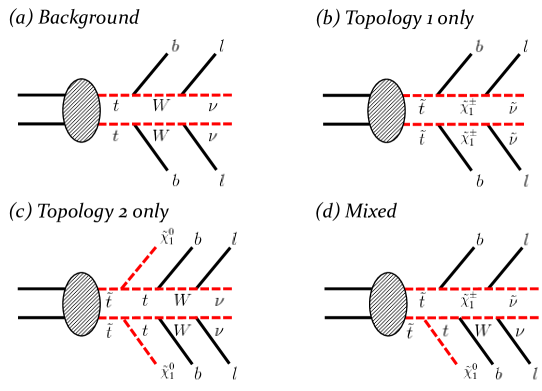
Specifically, we will consider how to discriminate between stop production, where both stops decay according to one of the topologies in Fig. 1, and the irreducible background from $t\bar{t}$ dilepton events. Fig. 2(a) illustrates the background event topology, while the corresponding three possible signal event topologies are depicted in Figs. 2(b-d). In all these processes, the observed final state consists of two $b$-jets, two opposite sign (OS) leptons, and MET, which makes it quite challenging to discover stops in this channel.

Note in particular that our analysis will allow for the mixed event topology of Fig. 2(d). This is because we shall not make any assumptions about the relative branching fraction between Topologies 1 and 2 in Fig. 1. If the two branching fractions are comparable, there is a sizable fraction of events of the type depicted in Fig. 2(d); their number benefits also from the combinatorial factor of 2 relative to the events in Fig. 2(b) or the events in Fig. 2(c).

Figure 3: The background event topology of Fig. 2(a) with the corresponding subsystems explicitly delineated. The blue dotted, green dot-dashed, and black solid lines indicate the subsystems $(a)$, $(b)$, and $(ab)$, respectively. See also Table 1.

1.3 On-shell constrained $M_{2}$ variables

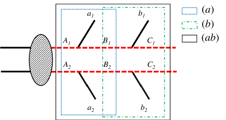
In this paper we investigate the benefit of the recently proposed on-shell constrained $M_{2}$ variables Barr:2011xt ; Mahbubani:2012kx ; Cho:2014naa in discriminating between the signal events of Fig. 2(b-d) and the main background shown in Fig. 2(a). The $M_{2}$ variables are the natural $3+1$-dimensional generalizations Barr:2011xt of the Cambridge $M_{T2}$ variable Lester:1999tx ; Barr:2003rg , which is already known as a useful tool for background suppression Barr:2009wu ; Allanach:2011ej ; Murayama:2011hj . Both $M_{2}$ and $M_{T2}$ were designed for events in which particles are pair produced and decay semi-invisibly. (I.e., some of the decay products are invisible.) The variables can then be computed for different subsystems in the event, or for the original event as a whole Burns:2008va . For example, in the case of the background $t\bar{t}$ events from Fig. 2(a), there are three possibilities, which are shown in Fig. 3. We shall follow the notation of Cho:2014naa and label these three possibilities as $(ab)$, $(a)$, and $(b)$.

In the spirit of many other kinematic variables such as $M_{T2}$ Lester:1999tx , $M_{2C}$ Ross:2007rm , and $M_{CT2}$ Cho:2009ve , the $M_{2}$ variables are obtained by minimizing some parent invariant mass with respect to the momenta of the invisible daughter particles. (The exact definition and basic properties of the constrained $M_{2}$ variables are reviewed in Sec. 2 below.) In the process of minimization, one may additionally impose certain kinematic constraints which follow from the hypothesized event topology. The main advantage of the $M_{2}$ class of variables is that, being $3+1$-dimensional, they allow one to incorporate all known kinematic constraints Mahbubani:2012kx ; Cho:2014naa . For example, $M_{T2}$ and $M_{CT2}$ are transverse variables, and the only constraint which can be used in their calculation is the MET constraint. On the other hand, in calculating an $M_{2}$ variable, one is free to impose additional mass shell conditions following either from a previous measurement (as in the case of $M_{2C}$) or from a theoretical hypothesis about the specific nature of the events, e.g. that the two decay chains in Fig. 3 are the same and thus $M_{A_{1}}=M_{A_{2}}$, $M_{B_{1}}=M_{B_{2}}$ and $M_{C_{1}}=M_{C_{2}}$.

The presence of additional on-shell constraints will generally increase the calculated value of $M_{2}$ — the more constraints there are, the larger the value of $M_{2}$. This simple observation will be at the center of our discussion below, and we shall use it in several different ways:

• The imposition of the additional constraints raises the value of $M_{2}$, distorting the shape of the $M_{2}$ distribution by increasing the populations of the higher $M_{2}$ bins. We can use this effect to increase the signal efficiency in those cases where the background $M_{2}$ distribution is bounded by an upper kinematic endpoint, while the signal $M_{2}$ distribution extends beyond this kinematic endpoint. This effect will be discussed and illustrated in Sec. 3 for signal events with Topology 1 only, and in Sec. 4 for signal events with Topology 2 only. In either case, the two top squarks decay identically, giving rise to the “symmetric” event topologies of Fig. 2(b) and Fig. 2(c), respectively.

• The kinematic variables $M_{T2}$ and $M_{2}$ were originally designed for symmetric events, and intended to be used for such events only. But what if the actual event is “asymmetric” and the two parent particles decay in a different manner, e.g., as in Fig. 2(d)? There are two possible approaches. First, one could suitably modify the definition of $M_{T2}$ in order to adapt it to an asymmetric case Barr:2009jv ; Konar:2009qr . This would still work, provided that both the signal and background have the same asymmetric event topology. However, what if the background events are symmetric (as in Fig. 2(a)), while the signal events are asymmetric (as in Fig. 2(d)) or vice versa? This case is the subject of Sec. 5, in which we shall advocate the use of the conventional “symmetric” on-shell constrained $M_{2}$ variables for this asymmetric case as well. As an illustration, we shall consider a particularly difficult scenario, when the kinematic endpoints of the symmetric events with Topology 1 (Fig. 2(b)) or Topology 2 (Fig. 2(c)) are too low and are both “buried” inside the background distribution. Nevertheless, when we compute the $M_{2}$ variables for the mixed event topology of Fig. 2(d), we shall find that the signal distribution does extend beyond the background endpoint. The reason for this apparent “endpoint violation” is simply the fact that when calculating $M_{2}$, we are applying the “wrong” constraints on the signal events, but the “correct” constraints on the background events.

• The benefit of the on-shell constrained $M_{2}$ variables is not limited only to events in which the background $M_{2}$ endpoint is violated. We can achieve additional separation of signal from background by studying the size of the shift caused by the application of the on-shell constraints. In Sec. 6 we shall find that this shift is generally larger for signal events with the mixed event topology of Fig. 2(d) when compared to the corresponding shift for background events. This observation is valid even for signal events which do not violate the background $M_{2}$ endpoint. The study presented in Sec. 6 also includes the effects of detector resolution and combinatorial backgrounds.

1.4 Précis

In this paper we put forth four ideas for stop discovery.

1. We propose to use the on-shell constrained $M_{2}$ variables from each of the three subsystems ($(a)$, $(b)$, and $(ab)$) Burns:2008va ; Bai:2013ema . Previous efforts described in the literature have relied mostly on the dileptonic $M_{T2}$ Plehn:2012pr ; Kilic:2012kw ; Chakraborty:2013moa ; Cho:2008cu .

2. We advocate the use of the on-shell constrained $(3+1)$-dimensional $M_{2}$ variables in place of their transverse cousin $M_{T2}$, due to their ability to “push” more signal events beyond the background endpoints, thus increasing the signal efficiency.

3. We also propose to use the difference between the on-shell constrained $M_{2}$ variable and its analogue $M_{T2}$ as an additional discriminator against the background.

4. We show that the on-shell constrained $M_{2}$ variable is able to specifically target the mixed signal event topology of Fig. 2(d) and salvage a certain fraction of signal events in difficult scenarios when more conventional cuts would fail.

2 Review of on-shell constrained $M_{2}$ variables

In this section we provide a brief review of on-shell constrained $M_{2}$ variables. Readers who are familiar with the terminology and notation of Ref. Cho:2014naa may skip directly to Sec. 3. We begin by reminding the reader that there exists a broad class of kinematic variables that are useful in the analysis of events with missing energy. These variables are defined in two steps Barr:2011xt :

• One first assumes a particular event topology consistent with the final state particles observed in the event.

• One then minimizes an invariant mass quantity in the hypothesized topology over the unknown invisible momenta, subject to certain kinematic constraints.

The best known example of such a variable is the usual transverse mass $M_{T}$,  Smith:1983aa ; Barger:1983wf , which applies to the simple case of one decay chain with a single invisible particle. Although a transverse quantity, $M_{T}$ can be thought of as the minimum value of the 3+1 dimensional invariant mass, consistent with the measured missing transverse momentum Barr:2011xt . This example is rather trivial in the sense that imposing the vector constraint of transverse momentum conservation already fixes the (transverse) components of the invisible particle momentum, and there is only one minimization left to do. A much more interesting case arises when there are two decay chains, with one invisible particle in each. Then the concept of $M_{T}$ is generalized to the stransverse mass, $M_{T2}$ Lester:1999tx , in which one finds the minimum, with respect to the momenta of invisible particles, of the maximum transverse mass of a given particle on either side of a (symmetric) decay topology, again subject to the constraint of total transverse momentum conservation.

The on-shell constrained $M_{2}$ variables described in Cho:2014naa are analogous to $M_{T2}$, with two main differences. First, the quantity being minimized is the four-dimensional invariant mass rather than the transverse mass (see also Ross:2007rm ; Barr:2011xt ; Mahbubani:2012kx ). Second, in addition to transverse momentum conservation, one is free to apply additional on-shell constraints which follow from the assumed event topology. For concreteness, let us use the event topology of Fig. 3 to illustrate the procedure of defining the different types of $M_{2}$ variables, denoted as

$$M_{2\sqcup\sqcup}(S;\tilde{m}).$$ (1)

Here $S\in\{(ab),(a),(b)\}$ denotes the subsystem under consideration, while $\sqcup$ is an index placeholder to be defined shortly.

Subsystem	Parents	Daughters	Relatives
$S$	$P_{i}$	$D_{i}$	$R_{i}$
$(ab)$	$\{A_{i}\}=\{t,\bar{t}\,\}$	$\{C_{i}\}=\{\nu,\bar{\nu}\,\}$	$\{B_{i}\}=\{W^{+},W^{-}\}$
$(a)$	$\{A_{i}\}=\{t,\bar{t}\,\}$	$\{B_{i}\}=\{W^{+},W^{-}\}$	$\{C_{i}\}=\{\nu,\bar{\nu}\,\}$
$(b)$	$\{B_{i}\}=\{W^{+},W^{-}\}$	$\{C_{i}\}=\{\nu,\bar{\nu}\,\}$	$\{A_{i}\}=\{t,\bar{t}\,\}$

Table 1: The roles played by different particles in the background process of $t\bar{t}$ production (Fig. 2(a)), for each of the three subsystems defined in Fig. 3.

According to the nomenclature of Cho:2014naa , depending on the subsystem being considered, the intermediate particles $A_{i}$, $B_{i}$, and $C_{i}$ fall into one of the following three categories (see Table 1):

• Daughters $D_{i}$. These are the invisible particles at the end of the decay chains in the subsystem under consideration. Following Cho:2014naa , we shall denote their 3-momenta by $\vec{q}_{1}$ and $\vec{q}_{2}$, respectively. The value of the $M_{2}$ variable (1) will be obtained by minimizing over all possible values of $\vec{q}_{1}$ and $\vec{q}_{2}$, consistent with the applied kinematic constraints. As usual, we shall take the daughters’ masses to be equal:

  $$M_{D_{1}}=M_{D_{2}}\equiv\tilde{m}$$ (2)

  and denote them with $\tilde{m}$, which will be an input parameter for the $M_{2}$ calculation.

• Parents $P_{i}$. These are the two particles at the top of the decay chains in the subsystem, and their masses will be subject to minimization over the invisible momenta in order to obtain the variable (1). When performing this minimization, in addition to the missing transverse momentum constraint

  $$\vec{q}_{1T}+\vec{q}_{2T}={\;/\!\!\!\!\vec{P}_{T}},$$ (3)

  we can additionally require that the two parent masses (when considered as functions of the invisible momenta) are the same:

  $$M^{2}_{P_{1}}(\vec{q}_{1},\tilde{m})=M^{2}_{P_{2}}(\vec{q}_{2},\tilde{m}).$$ (4)

  The presence (or absence) of this constraint is indicated by the first _⊔ index in (1), which takes value $C$ if the constraint is applied, and $X$ otherwise:

  $$M_{2C\sqcup}(S;\tilde{m}) \equiv \min_{\begin{subarray}{c}\vec{q}_{1},\vec{q}_{2}\\ \vec{q}_{1T}+\vec{q}_{2T}={\;/\!\!\!\!\vec{P}_{T}}\\ M^{2}_{P_{1}}(\vec{q}_{1},\tilde{m})=M^{2}_{P_{2}}(\vec{q}_{2},\tilde{m})\end{subarray}}\left\{M_{P_{1}}(\vec{q}_{1},\tilde{m})\right\},$$ (5)

  $$M_{2X\sqcup}(S;\tilde{m}) \equiv \min_{\begin{subarray}{c}\vec{q}_{1},\vec{q}_{2}\\ \vec{q}_{1T}+\vec{q}_{2T}={\;/\!\!\!\!\vec{P}_{T}}\end{subarray}}\left\{\max\left[M_{P_{1}}(\vec{q}_{1},\tilde{m}),M_{P_{2}}(\vec{q}_{2},\tilde{m})\right]\right\}.$$ (6)

• Relatives $R_{i}$. As shown in Table 1, the relatives are the remaining particles in the event topology — they are neither parents nor daughters. Depending on the subsystem, relatives can appear either inside or outside the subsystem. Their masses can also be written as functions of the respective daughters’ momenta, so by requiring equal masses for the relative particles,

  $$M_{R_{1}}^{2}(\vec{q}_{1},\tilde{m})=M_{R_{2}}^{2}(\vec{q}_{2},\tilde{m}),$$ (7)

  we are, in effect, imposing an additional constraint on the minimization over the invisible momenta $\vec{q}_{i}$. The applicability of the constraint (7) will be indicated by the second _⊔ index in (1): as before, it will be equal to $C$ if the constraint (7) is applied and $X$ otherwise. Altogether, therefore, we have four possible $M_{2}$ variables:

  $$M_{2CC}(S;\tilde{m}) \equiv \min_{\begin{subarray}{c}\vec{q}_{1},\vec{q}_{2}\\ \vec{q}_{1T}+\vec{q}_{2T}={\;/\!\!\!\!\vec{P}_{T}}\\ M_{P_{1}}^{2}(\vec{q}_{1},\tilde{m})=M_{P_{2}}^{2}(\vec{q}_{2},\tilde{m})\\ M_{R_{1}}^{2}(\vec{q}_{1},\tilde{m})=M_{R_{2}}^{2}(\vec{q}_{2},\tilde{m})\end{subarray}}\left\{M_{P_{1}}(\vec{q}_{1},\tilde{m})\right\},$$ (8)

  $$M_{2CX}(S;\tilde{m}) \equiv \min_{\begin{subarray}{c}\vec{q}_{1},\vec{q}_{2}\\ \vec{q}_{1T}+\vec{q}_{2T}={\;/\!\!\!\!\vec{P}_{T}}\\ M_{P_{1}}^{2}(\vec{q}_{1},\tilde{m})=M_{P_{2}}^{2}(\vec{q}_{2},\tilde{m})\end{subarray}}\left\{M_{P_{1}}(\vec{q}_{1},\tilde{m})\right\},$$ (9)

  $$M_{2XC}(S;\tilde{m}) \equiv \min_{\begin{subarray}{c}\vec{q}_{1},\vec{q}_{2}\\ \vec{q}_{1T}+\vec{q}_{2T}={\;/\!\!\!\!\vec{P}_{T}}\\ M_{R_{1}}^{2}(\vec{q}_{1},\tilde{m})=M_{R_{2}}^{2}(\vec{q}_{2},\tilde{m})\end{subarray}}\left\{\max\left[M_{P_{1}}(\vec{q}_{1},\tilde{m}),M_{P_{2}}(\vec{q}_{2},\tilde{m})\right]\right\},$$ (10)

  $$M_{2XX}(S;\tilde{m}) \equiv \min_{\begin{subarray}{c}\vec{q}_{1},\vec{q}_{2}\\ \vec{q}_{1T}+\vec{q}_{2T}={\;/\!\!\!\!\vec{P}_{T}}\end{subarray}}\left\{\max\left[M_{P_{1}}(\vec{q}_{1},\tilde{m}),M_{P_{2}}(\vec{q}_{2},\tilde{m})\right]\right\}.$$ (11)

The definitions (8-11) should be contrasted to the analogous definition of the Cambridge $M_{T2}$ variable

$$M_{T2}(S;\tilde{m})\equiv\min_{\begin{subarray}{c}\vec{q}_{1T},\vec{q}_{2T}\\ \vec{q}_{1T}+\vec{q}_{2T}={\;/\!\!\!\!\vec{P}_{T}}\end{subarray}}\left\{\max\left[M_{TP_{1}}(\vec{q}_{1T},\tilde{m}),M_{TP_{2}}(\vec{q}_{2T},\tilde{m})\right]\right\},$$ (12)

where only the transverse components $\vec{q}_{iT}$ are used, and the objective function (the function that is minimized) is the larger of the two transverse masses of the parents.

The main goal of this paper is to investigate and contrast the ability of the variables (8-12) to discriminate between the $t\bar{t}$ background of Fig. 2(a) and the three types of stop signal events of Fig. 2(b-d). We shall consider the respective variables for all three subsystems of Fig. 3. Since we know the mass spectrum for the background event topology, we shall choose the test mass $\tilde{m}$ to be equal to the correct, SM value for the respective daughter particle. In particular,

• In subsystem $(ab)$, the parent particle is the top quark; the daughter particle is the neutrino, whose mass is taken to vanish ($\tilde{m}=0$). The other, “relative”, particle is the $W^{\pm}$ boson. Then for background events, all 5 variables (8-12) are bounded from above by the top mass:

  $$M_{T2}(ab;0),M_{2XX}(ab;0),M_{2CX}(ab;0),M_{2XC}(ab;0),M_{2CC}(ab;0)\leq m_{t},$$ (13)

  while for signal events, this bound can be violated.

• In subsystem $(a)$, the parent particle is again the top quark. The daughter particle is now the $W^{\pm}$ boson, with mass $\tilde{m}=m_{W}$. The relative particles are the two neutrinos, which in this case appear downstream outside the subsystem. For background events, the variables are again bounded by the top mass

  $$M_{T2}(a;m_{W}),M_{2XX}(a;m_{W}),M_{2CX}(a;m_{W}),M_{2XC}(a;m_{W}),M_{2CC}(a;m_{W})\leq m_{t}.$$ (14)

• In subsystem $(b)$ the parent particles are the $W^{\pm}$ bosons, the daughter particles are the two neutrinos with mass $\tilde{m}=0$, and the relative particles are the top quarks appearing upstream outside the subsystem. The background events obey

  $$M_{T2}(b;0),M_{2XX}(b;0),M_{2CX}(b;0),M_{2XC}(b;0),M_{2CC}(b;0)\leq m_{W}.$$ (15)

In principle, each of the bounds (13-15) allows us to cut $100\%$ of the $t\bar{t}$ background events by removing events with values of the respective subsystem $M_{2}$ or $M_{T2}$ variable below the appropriate threshold (“high pass cut”). Therefore, as far as just the background is concerned, we have 15 alternative choices for reducing it, and they should perform comparably well. The differences between the five variables (8-12) begin to emerge when we consider the effect of such a high pass cut on signal events. It has been shown Cho:2014naa that the variables (8-12) obey the following hierarchy

$$M_{T2}(S;\tilde{m})=M_{2XX}(S;\tilde{m})=M_{2CX}(S;\tilde{m})\leq M_{2XC}(S;\tilde{m})\leq M_{2CC}(S;\tilde{m})$$ (16)

for any subsystem $S$ and any value of $\tilde{m}$. We should therefore expect the distributions of $M_{2XC}$ and $M_{2CC}$ to be more populated at higher values and in particular near their endpoints. As a result, signal events are more likely to pass if the cut is applied on the additionally constrained variables, $M_{2XC}$ and $M_{2CC}$, as opposed to the less constrained variables $M_{T2}$, $M_{2XX}$, and $M_{2CX}$. This expectation is borne out by the explicit studies below. The property (16) offers an opportunity to increase the sensitivity of the LHC experiments to the presence of stop signals of the type described in Fig. 2(b-d).

3 $M_{2}$ endpoint study for topology 1

We begin by studying the effectiveness of the on-shell constrained subsystem $M_{2}$ variables in the case where both stops in the signal event decay according to Topology 1. This yields the event topology pictured in Fig. 2(b). The background, as always in this paper, consists of dileptonic top production and is shown in Fig. 2(a). We remind the reader that when applied to background events, all of the on-shell constrained subsystem $M_{2}$ variables (as well as $M_{T2}$) exhibit very well-defined kinematic endpoints given by Eqs. (13-15). Therefore, the effectiveness of the $M_{2}$ variables in identifying signal events is determined by how many signal events violate the bounds (13-15).

The signal events considered in this section (those of Fig. 2(b)) have exactly the same topology as the background. Therefore, when applied to signal events, the $M_{2}$ variables will have well-defined upper kinematic endpoints as well. The precise value of those endpoints will depend on the underlying signal mass spectrum, i.e., on the true values of the stop mass $m_{\tilde{t}}$, the chargino mass $m_{\tilde{\chi}^{\pm}}$, and the sneutrino mass $m_{\tilde{\nu}}$. For any given point $\{m_{\tilde{t}},m_{\tilde{\chi}^{\pm}},m_{\tilde{\nu}}\}$ in the mass parameter space, using the formulas given in Ref. Burns:2008va , one can compute the expected $M_{2}$ kinematic endpoints for the signal, in each of the three subsystems $(ab)$, $(a)$, and $(b)$. Depending on the SUSY mass spectrum, some, all, or none of these signal endpoints will exceed the corresponding background endpoints. In the second half of this section, we shall illustrate each of these three scenarios with specific study points. But first we shall analyze the relevant mass parameter space and categorize the different regions, which are defined by the location of the signal endpoints relative to the background endpoints. This will be the subject of the next subsection.

3.1 Anatomy of the mass parameter space for Topology 1

In order to divide the stop-chargino-sneutrino mass parameter space into regions, we start with the analytical expressions for the $M_{T2}$ signal endpoints Cho:2007qv ; Cho:2007dh ; Burns:2008va . (The endpoints for the corresponding $M_{2\sqcup\sqcup}$ variables are given by the exact same expressions Cho:2014naa .)

$$M_{T2}^{max}(ab;\tilde{m}=0) = \frac{m^{2}_{\tilde{t}}-m^{2}_{\tilde{\nu}}}{m_{\tilde{t}}},$$ (17)

$$M_{T2}^{max}(a;\tilde{m}=m_{W}) = \frac{m^{2}_{\tilde{t}}-m^{2}_{\tilde{\chi}^{\pm}}}{2m_{\tilde{t}}}+\sqrt{\left(\frac{m^{2}_{\tilde{t}}-m^{2}_{\tilde{\chi}^{\pm}}}{2m_{\tilde{t}}}\right)^{2}+m_{W}^{2}},$$ (18)

$$M_{T2}^{max}(b;\tilde{m}=0) = \sqrt{\frac{(m^{2}_{\tilde{t}}-m^{2}_{\tilde{\nu}})(m^{2}_{\tilde{\chi}^{\pm}}-m^{2}_{\tilde{\nu}})}{m^{2}_{\tilde{t}}}}.$$ (19)

Now combining, e.g., Eqs. (13) and (17), we find that for the variables in the $(ab)$ subsystem, the signal endpoints exceed the background endpoints if

$$\frac{m^{2}_{\tilde{t}}-m^{2}_{\tilde{\nu}}}{m_{\tilde{t}}}>m_{t}.$$ (20)

The corresponding region is delineated by the solid black line in Fig. 4, which shows a slice through the 3-dimensional mass parameter space for fixed $m_{\tilde{\nu}}=110$ GeV. For convenience we choose to represent the remaining two degrees of freedom as the mass differences $m_{\tilde{\chi}^{\pm}}-m_{\tilde{\nu}}$ and $m_{\tilde{t}}-m_{\tilde{\chi}^{\pm}}$. The region satisfying the condition (20) is above and to the right of the solid black line in Fig. 4. If the SUSY mass spectrum happens to be in this region, the mass splitting between the stop and the sneutrino is sufficiently large to cause some number of signal events to “leak” beyond the background endpoint (13). This means that the subsystem $(ab)$ variables are promising variables to cut on in order to separate signal from background.

Figure 4: The division of stop-chargino-sneutrino mass parameter space into regions, which are defined by which of the background endpoints are violated by signal events in which both stops decay according to Topology 1. The sneutrino mass has been set to $110$ GeV. The four study points considered later in this section are also indicated.

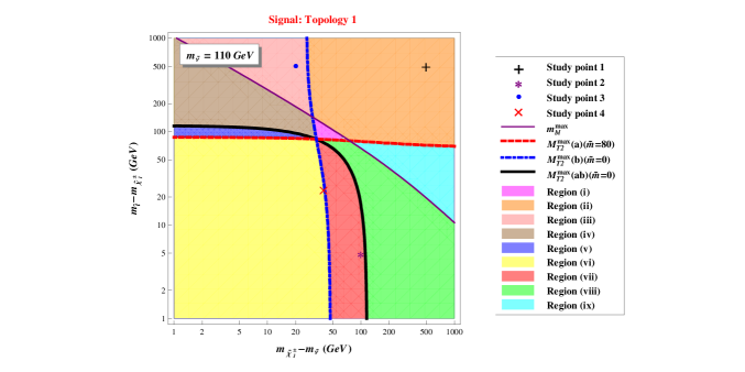
We can apply similar reasoning to the invariant mass variables in subsystems $(a)$ and $(b)$. For example, comparing Eqs. (14) and (18), we find that the bound (14) applicable to background events will be violated if the mass spectrum is such that

$$\frac{m^{2}_{\tilde{t}}-m^{2}_{\tilde{\chi}^{\pm}}}{m_{\tilde{t}}}>\frac{m^{2}_{t}-m^{2}_{W}}{m_{t}}.$$ (21)

The corresponding region extends above the red dashed line in Fig. 4. Finally, the condition for violating the background endpoints in subsystem $(b)$ follows from Eqs. (15) and (19):

$$\frac{(m^{2}_{\tilde{t}}-m^{2}_{\tilde{\nu}})(m^{2}_{\tilde{\chi}^{\pm}}-m^{2}_{\tilde{\nu}})}{m^{2}_{\tilde{t}}}>m_{W}^{2}.$$ (22)

The region where this condition is satisfied is located to the right of the blue dot-dashed line in Fig. 4.

For completeness, we shall also consider the variable $m_{bl}$, the invariant mass of the lepton and $b$ quark from a given branch of the decay. The endpoint of this quantity for signal events is given by

$$m_{b\ell}^{max}=\sqrt{\frac{(m_{\tilde{t}}^{2}-m_{\tilde{\chi}^{\pm}}^{2})(m_{\tilde{\chi}^{\pm}}^{2}-m_{\tilde{\nu}}^{2})}{m_{\tilde{\chi}^{\pm}}^{2}}},$$ (23)

while background events will obey the bound

$$m_{b\ell}\leq\sqrt{m_{t}^{2}-M_{W}^{2}}.$$ (24)

Therefore the condition for violating the background $m_{b\ell}$ endpoint is

$$\frac{(m_{\tilde{t}}^{2}-m_{\tilde{\chi}^{\pm}}^{2})(m_{\tilde{\chi}^{\pm}}^{2}-m_{\tilde{\nu}}^{2})}{m_{\tilde{\chi}^{\pm}}^{2}}>m_{t}^{2}-M_{W}^{2}.$$ (25)

The corresponding region is found above and to the right of the diagonal magenta thin solid line in Fig. 4.

	$m_{b\ell}$	$M_{T2}(ab)$	$M_{T2}(a)$	$M_{T2}(b)$
Region	endpoint	endpoint	endpoint	endpoint
	violation	violation	violation	violation
i	No	Yes	Yes	Yes
ii	Yes	Yes	Yes	Yes
iii	Yes	Yes	Yes	No
iv	No	Yes	Yes	No
v	No	No	Yes	No
vi	No	No	No	No
vii	No	No	No	Yes
viii	No	Yes	No	Yes
ix	Yes	Yes	No	Yes

Table 2: The regions of stop-chargino-sneutrino mass space, as depicted in Fig. 4. The four columns describe whether in the given region, the specified background endpoint can be violated by signal events where both stops decay according to Topology 1.

The conditions implied by Eqs. (20-22) and (25) divide the mass parameter space of Fig. 4 into nine distinct color-coded regions, which are defined in Table 2. It is easy to verify analytically that the boundaries of the three regions defined by conditions (20-22), i.e., the red, blue, and black curves in Fig. 4, cross at a single point. For any given sneutrino mass, $m_{\tilde{\nu}}$, the values of the stop mass, $m_{\tilde{t}}$, and the chargino mass, $m_{\tilde{\chi}^{\pm}}$, corresponding to the triple crossing point are found from the relations

$$\frac{m^{2}_{\tilde{t}}-m^{2}_{\tilde{\nu}}}{m_{\tilde{t}}}=m_{t},\qquad\frac{m_{\tilde{\chi}^{\pm}}^{2}-m_{\tilde{\nu}}^{2}}{m_{\tilde{t}}}=\frac{m_{W}^{2}}{m_{t}}.$$

The map in Fig. 4 serves a dual purpose. First, it singles out the regions which might be easier to discover, as well as the regions which may pose challenges. Second, within each region, it identifies the variables which might be useful in the analysis (see Table 2). For example, in region ii, the mass spectrum is sufficiently split, and all four variables exhibit endpoint violations for signal events. This in turn suggests that separating signal from background should be relatively easy, since we can use any of the four types of invariant mass variables in Table 2 to suppress the background without much signal loss. To illustrate the expected phenomenology of region ii, in Sec. 3.2 we shall analyze in detail a specific study point from this region. Its mass spectrum is given in Table 3 and its exact location on the map of Fig. 4 is marked with a black cross ($+$).

Study Point	Stop Mass	Chargino Mass	Sneutrino Mass	Region
1	$1110$ GeV	$610$ GeV	$110$ GeV	ii
2	$215$ GeV	$210$ GeV	$110$ GeV	vii
3	$630$ GeV	$130$ GeV	$110$ GeV	iii
4	$174$ GeV	$150$ GeV	$110$ GeV	vi

Table 3: The stop, chargino, and sneutrino masses for the four study points considered in this section, as well as the region of mass parameter space from Fig. 4 that contains each point.

In all but one of the remaining regions of Fig. 4, some of the endpoints are violated while others are not, thus some variables are expected to perform better than others. We pick two representative study points in regions vii and iii and study them in Secs. 3.3 and 3.4, respectively. In Fig. 4, these two study points are marked with the magenta asterisk $(\ast)$ and the blue circle ($\bullet$). The corresponding mass spectra are also listed in Table 3.

Finally, region vi deserves a special mention, since it represents a particularly challenging scenario. Here none of the four types of invariant mass variables exhibits an endpoint violation, and the signal events are populating the same kinematic region as the background events. Our fourth study point in Table 3 (denoted in Fig. 4 with the red ($\times$) symbol) belongs to this challenging region and is considered in Sec. 3.5.

3.2 Study point 1: split spectrum in region ii

In this section we shall illustrate the properties of region ii in Fig. 4 with the study point 1 which is marked with the black ($+$) symbol. As seen in Table 3, this study point has a widely split spectrum; both mass differences $m_{\tilde{t}}-m_{\tilde{\chi}^{\pm}}$ and $m_{\tilde{\chi}^{\pm}}-m_{\tilde{\nu}}$ are $500$ GeV.

Figure 5: Signal (thick red lines) and background (thin blue lines) distributions for the subsystem variables $M_{T2}(S;\tilde{m})$ (dashed lines) and $M_{2CC}(S;\tilde{m})$ (solid lines). We show results for each of the three possible subsystems: $S=(ab)$ (upper left panel), $S=(a)$ (upper right panel), and $S=(b)$ (lower left panel). The lower right panel shows the analogous distributions for the invariant mass $m_{b\ell}$. The signal events are for study point 1 ($m_{\tilde{t}}=1110$ GeV, $m_{\tilde{\chi}^{\pm}}=610$ GeV and $m_{\tilde{\nu}}=110$ GeV) and have the event topology shown in Fig. 2(b).

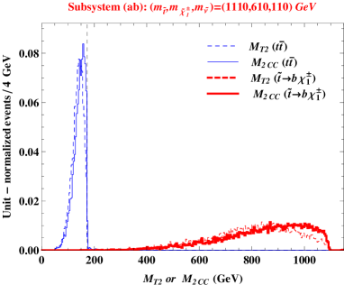
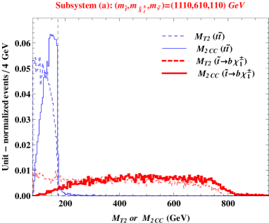
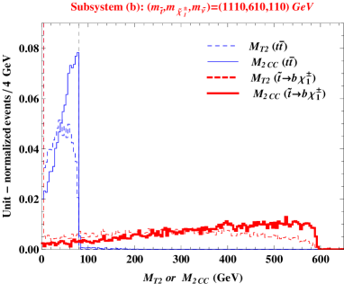
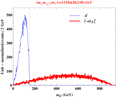
One can therefore expect that the signal distributions for our invariant mass variables will extend well beyond the corresponding background distributions. This is confirmed in Fig. 5, where we plot distributions for signal events (red lines) and background events (blue lines) for $M_{T2}(S;\tilde{m})$ (dashed lines), $M_{2CC}(S;\tilde{m})$ (solid lines), and $m_{b\ell}$. As always in this section, the signal events are assumed to have the symmetric event topology of Fig. 2(b), i.e., both stops decay according to Topology 1. Fig. 5 shows results for all three subsystems: $S=(ab)$ (upper left panel), $S=(a)$ (upper right panel) and $S=(b)$ (lower left panel). In each case, the trial mass $\tilde{m}$ for the respective daughter particle has been set to the correct value for SM events, as explained in more detail in Appendix A. In each panel of Fig. 5, the vertical dashed line marks the location of the kinematic endpoint for background events, as given by Eqs. (13-15) and (24). As expected, the blue (background) distributions always obey these kinematic endpoints. (The figure has been constructed using parton-level events with no detector modeling or combinatorial backgrounds — these effects will be added later on in Sec. 6.)

On the other hand, the signal events, shown in red, significantly violate the endpoints. In fact, for all four variables considered in Fig. 5, the vast majority of signal events violate the background endpoints. This is also to be expected, since study point 1 was chosen specifically in region ii, where all four endpoints are expected to be violated (see Table 2). This also means that discovery (or exclusion) for this study point should be relatively straightforward.

We have noted above that, on an event by event basis,

$$M_{T2}(S;\tilde{m})\leq M_{2CC}(s;\tilde{m}).$$ (26)

This is confirmed in Fig. 5, where the (solid line) $M_{2CC}$ distributions can be seen to be somewhat harder than the respective $M_{T2}$ dashed line distributions. As a result, cutting on $M_{2CC}$ instead of $M_{T2}$ will result in a slightly higher signal efficiency. (The effect is most easily seen for subsystems $(a)$ and $(b)$.)

Figure 6: Signal (thick red lines) and background (thin blue lines) distributions of some standard variables for study point 1 ($m_{\tilde{t}}=1110$ GeV, $m_{\tilde{\chi}^{\pm}}=610$ GeV and $m_{\tilde{\nu}}=110$ GeV): the missing transverse energy $MET$ (left panel), the lepton transverse momentum $p_{T,\ell}$ (middle panel), and the $b$-quark transverse momentum $p_{T,b}$ (right panel).

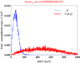
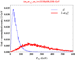
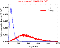
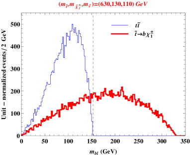
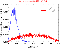
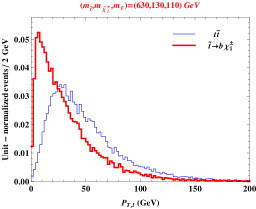
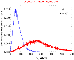
While the variables shown in Fig. 5 already allow study point 1 to be discovered or ruled out rather trivially, the same can be accomplished with more conventional variables like the missing transverse energy ($MET$), the lepton transverse momentum $p_{T,\ell}$, or the $b$-quark transverse momentum $p_{T,b}$, whose distributions for study point 1 are plotted in Fig. 6. In all three cases, even though the background distribution does not exhibit a strict endpoint, the signal and background distributions are very well separated, so the signal can be easily isolated. Furthermore, as we can measure four endpoints in Fig. 5 and there are only three input mass parameters, full mass reconstruction in this case is also possible Burns:2008va . In conclusion, the analysis of study point 1 demonstrates that region ii is “easy” in the sense that the experimenter has a plethora of useful tools available for a discovery. It is therefore of interest to consider the other, more challenging, regions of Fig. 4.

3.3 Study point 2: soft $b$-jets in region vii

Our second example is in region vii, in which only the variables in subsystem $(b)$ have endpoint violations. The mass spectrum for study point 2 is given in Table 3. We notice the relative degeneracy between the stop and chargino masses, which causes the endpoints of the signal $M_{T2}(a)$ and $m_{b\ell}$ distributions to be relatively low. (See Eqs. (18) and (23).) In addition, the sneutrino mass has been chosen so that the signal endpoint (17) of the $M_{T2}(ab)$ variable is also below the standard model expectation of (13). This leaves the $M_{T2}(b)$ variable as the only viable alternative in region vii.

Figure 7: The same as Fig. 5, but with signal events for study point 2 ($m_{\tilde{t}}=215$ GeV, $m_{\tilde{\chi}^{\pm}}=210$ GeV and $m_{\tilde{\nu}}=110$ GeV).

Figure 8: The same as Fig. 6, but for signal events for study point 2 ($m_{\tilde{t}}=215$ GeV, $m_{\tilde{\chi}^{\pm}}=210$ GeV and $m_{\tilde{\nu}}=110$ GeV).

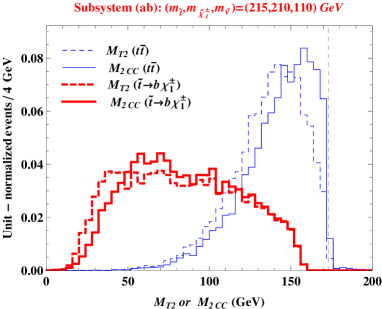
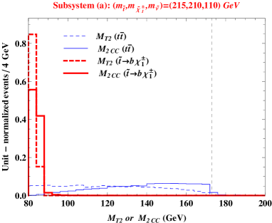
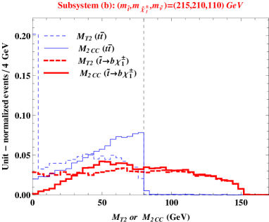
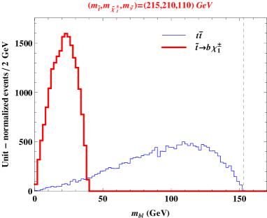
These observations are illustrated in Fig. 7 where we plot the relevant invariant mass distributions for study point 2 using the same conventions as in Fig. 5 above. Again, we assume that all signal events have the event topology shown in Fig. 2(b), i.e., both stops decay according to Topology 1. Fig. 7 confirms that $M_{T2}(b)$ is a good variable to cut on: placing a high pass cut with threshold just above $m_{t}$ would eliminate all of the background, while leaving almost half of the signal. To determine the optimal value of the threshold and the effectiveness of the cut requires realistic detector simulation (see Sec. 6), but it is clear that such a cut will often be useful. This observation is not new — the variable $M_{T2}(b)$ has been discussed in the literature under various names, e.g., $M_{T2}^{(210)}$ Burns:2008va and dileptonic $M_{T2}$ Plehn:2012pr ; Kilic:2012kw ; Chakraborty:2013moa ; Cho:2008cu . Here we would like to contrast $M_{T2}(b)$ to the alternative on-shell constrained variable $M_{2CC}(b)$. The advantage of the latter is the slightly higher signal efficiency. On the other hand, the advantage of the traditional $M_{T2}$ is its simplicity — in its calculation, one does not have to identify the $b$-jets, thus, one avoids combinatorial ambiguities and the additional penalty due to $b$-tagging.

Note that the signal and background distributions for the other three variables in Fig. 7: $M_{T2}(ab)$, $M_{T2}(a)$, and $m_{b\ell}$, also appear to be quite different, so one might wonder whether they could be useful if the cut were inverted (i.e., if one performs a low pass cut). However, we expect other background processes besides $t\bar{t}$ to contribute events at low values and swamp the signal Barr:2009wu ; Allanach:2011ej ; Murayama:2011hj . Such backgrounds may not be as well-understood, which is why in this study we shall only consider high pass cuts on the invariant mass variables.

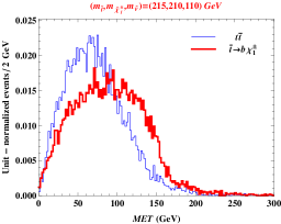
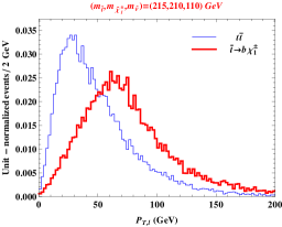
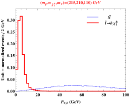
Having identified $M_{T2}(b)$ and $M_{2CC}(b)$ as promising variables, one might wonder how the more conventional variables would perform in this case. In Fig. 8, we show parton-level signal and background distributions for study point 2 for the three more traditional variables considered in Fig. 6: $MET$, $p_{T,\ell}$, and $p_{T,b}$. Since the stop-chargino mass splitting is rather small, the $b$-jets are quite soft and would often not be reconstructed. On the other hand, the $MET$ and $p_{T,\ell}$ distributions show some separation between signal and background, but the separation is less clear than we observed in the case of $M_{T2}(b)$ (the lower left panel of Fig. 5). Therefore, placing cuts on $MET$ and $p_{T,\ell}$ would not be as effective as cutting on $M_{T2}(b)$.

3.4 Study point 3: soft leptons in region iii

Our next example illustrates the complementarity of the subsystem invariant mass variables. In the previous subsection (3.3), we considered a signal study point with soft $b$-jets and relatively hard leptons, as seen in Fig. 8. Now we shall discuss the opposite situation, when the leptons are relatively soft, while the jets are hard. For this purpose, we focus on study point 3 in region iii, where according to Table 2 we expect endpoint violations for $M_{T2}(ab)$, $M_{T2}(a)$, and $m_{b\ell}$.

Figure 9: The same as Fig. 5, but with signal events for study point 3 ($m_{\tilde{t}}=630$ GeV, $m_{\tilde{\chi}^{\pm}}=130$ GeV and $m_{\tilde{\nu}}=110$ GeV).

Figure 10: The same as Fig. 6, but for signal events for study point 3 ($m_{\tilde{t}}=630$ GeV, $m_{\tilde{\chi}^{\pm}}=130$ GeV and $m_{\tilde{\nu}}=110$ GeV).

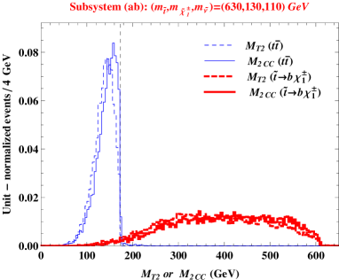
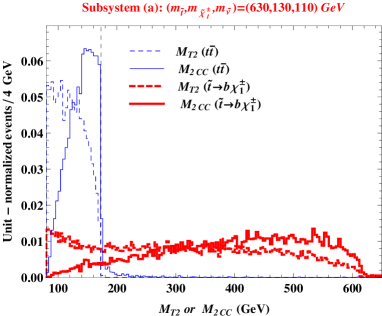
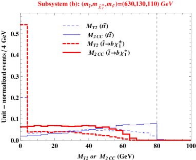
This feature is demonstrated in Fig. 9, where we again compare the signal and background distributions for the same four types of variables as in Figs. 5 and 7. We see that this time, as expected, the dilepton $M_{T2}$ variable ($M_{T2}(b)$ in our notation) is suboptimal; due to the softness of the leptons, the signal $M_{T2}(b)$ and $M_{2CC}(b)$ distributions lie entirely within the background region. On the other hand, the other three variables perform very well, unlike the case in Sec. 3.3. In particular, the subsystem $(ab)$ variables alone could possibly remove the background with virtually no loss of signal. The subsystem $(a)$ variables are also promising; the use of $M_{2CC}(a)$ seems slightly more effective than the use of $M_{T2}(a)$. Finally, the usual invariant mass, $m_{b\ell}$, allows one to separate signal and background, but the signal loss is more significant for this variable.

The lesson from Figs. 7 and 9 is that in order to efficiently probe the full mass parameter space of Fig. 4, one would have to design an analysis which utilizes the full complement of subsystem invariant mass variables, since different variables are optimal in different regions. Of course, one should not overlook the more conventional variables. In Fig. 10 we show the signal and background distributions of $MET$, $p_{T,\ell}$, and $p_{T,b}$ for study point 3. As expected, the lepton $p_{T}$ distribution for the signal is rather soft, but the signal distributions for both $MET$ and $p_{T,b}$ have long tails which extend to the right of the bulk of the corresponding background distribution. This suggests that $MET$ and $p_{T,b}$ could also play a useful role in the analysis.

3.5 Study point 4: a difficult case in region vi

Our final example for the signal event topology of Fig. 2(b) is a study point in the most challenging region, vi, where no endpoint violations should occur. The mass spectrum for study point 4 is given in Table 3, and the resulting signal and background distributions are displayed in Figs. 11 and 12.

Figure 11: The same as Fig. 5, but with signal events for study point 4 ($m_{\tilde{t}}=174$ GeV, $m_{\tilde{\chi}^{\pm}}=150$ GeV and $m_{\tilde{\nu}}=110$ GeV).

Figure 12: The same as Fig. 6, but for signal events for study point 4 ($m_{\tilde{t}}=174$ GeV, $m_{\tilde{\chi}^{\pm}}=150$ GeV and $m_{\tilde{\nu}}=110$ GeV).

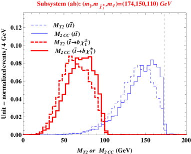
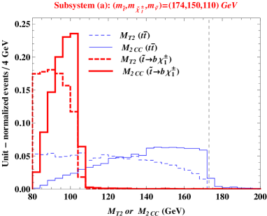
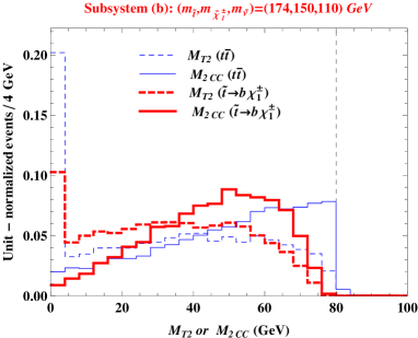
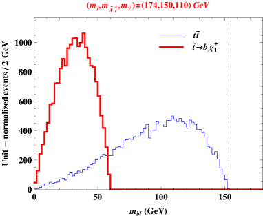
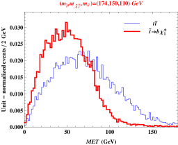
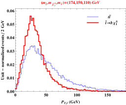
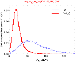
Discovery is clearly challenging in this scenario, as the $b$-jets will be quite soft, while the lepton $p_{T}$ and $MET$ distributions for the signal are very similar to those for the background. The invariant mass variables in Fig. 11 are not particularly helpful either, since the kinematic endpoints of the signal distributions are always below those of the background. Whether stops can be discovered at study point 4 thus remains an open question, which we shall revisit in Sec. 5.

4 $M_{2}$ endpoint study for Topology 2

In this section we shall focus on the other symmetric signal event topology in Fig. 2(c), when both stops decay according to Topology 2 in Fig. 1(b). The on-shell constrained invariant mass variables discussed in the previous section will be useful here as well, since they were constructed with the background topology in mind, which has not changed. Even though the signal event topology is now more complicated (there are two invisible particles in each decay chain), the signal distributions still exhibit kinematic endpoints. We find that the $M_{T2}$ endpoints are given by (see, e.g., Mahbubani:2012kx )

$$M_{T2}^{max}(ab;\tilde{m}=0) = 2\,C_{+}(m_{t},m_{\nu}),$$ (27)

$$M_{T2}^{max}(a;\tilde{m}=m_{W}) = C_{+}(m_{t},m_{W})+\sqrt{C^{2}_{+}(m_{t},m_{W})+m^{2}_{W}},$$ (28)

$$M_{T2}^{max}(b;\tilde{m}=0) = 2\,\sqrt{C_{+}(m_{W},m_{\nu})\,\left[C_{+}(m_{W},m_{\nu})-C_{-}(m_{t},m_{W})\right]},$$ (29)

where

$$C_{\pm}(x,y) \equiv \frac{x^{2}-y^{2}}{4\,m_{\tilde{t}}\,x^{2}}\,\left\{m^{2}_{\tilde{t}}+m^{2}_{t}-m^{2}_{\tilde{\chi}^{0}}\pm\sqrt{\lambda(m^{2}_{\tilde{t}},m^{2}_{t},m^{2}_{\tilde{\chi}^{0}})}\right\},$$ (30)

$$\lambda(x,y,z) \equiv x^{2}+y^{2}+z^{2}-2xy-2yz-2zx.$$ (31)

Upon careful examination of Eqs. (27-29), one can show that these kinematic endpoints are always above the corresponding background endpoints (13-15), as long as the channel $\tilde{t}\to t\tilde{\chi}^{0}$ is open (i.e., the decay is kinematically allowed). As we move close to the threshold for $\tilde{t}\to t\tilde{\chi}^{0}$, the signal kinematic endpoints (27-29) converge to the corresponding SM values (13-15), and discovery becomes very challenging. In this section, therefore, we shall consider two study points: one above this threshold and one at threshold. The mass spectra for those study points are listed in Table 4.

Study Point	Stop Mass	Neutralino Mass
5	$300$ GeV	$100$ GeV
6	$174$ GeV	$0$ GeV

Table 4: The stop and neutralino masses for the two study points considered in this section.

4.1 Study point 5: a case above the $\tilde{t}\to t\tilde{\chi}^{0}$ threshold

We first discuss study point 5, where the mass splitting is large enough that the decay $\tilde{t}\to t\tilde{\chi}^{0}$ is open, and the resulting top quark is on-shell. The corresponding kinematic distributions are shown in Figs. 13 and 14.

Figure 13: The same as Fig. 5, but for signal events with the event topology of Fig. 2(c) for study point 5 ($m_{\tilde{t}}=300$ GeV and $m_{\tilde{\chi}^{0}}=100$ GeV).

Figure 14: The same as Fig. 6, but for signal events with the event topology of Fig. 2(c) for study point 5 ($m_{\tilde{t}}=300$ GeV and $m_{\tilde{\chi}^{0}}=100$ GeV).

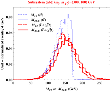
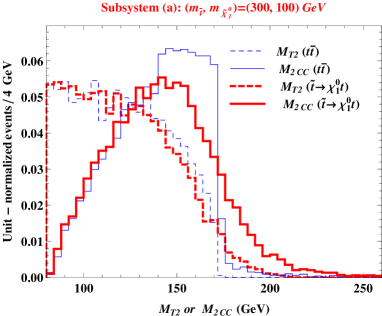
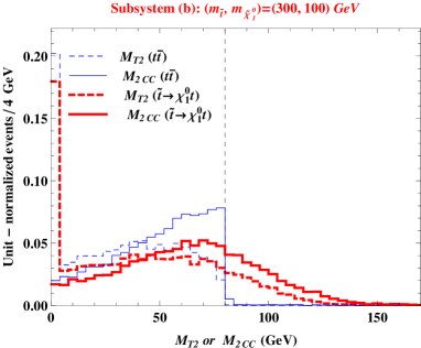
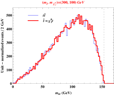
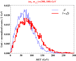
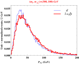
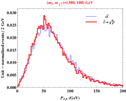
It is clear that this is already a challenging case — the signal and background distributions for the “conventional” variables in Fig. 14 are rather similar. The jet and lepton $p_{T}$ spectra are governed by the known mass differences between the SM particles $t$, $W^{\pm}$, and $\nu$, thus, there is very little distinction between the signal and background $p_{T}$ distributions. Similarly, the $m_{b\ell}$ distribution in Fig. 13 is the same for signal and background. The $MET$ distribution in Fig. 14 is slightly harder for the signal, due to the presence of two additional invisible particles. However, the effect is very small and hence unlikely to be useful in practice.

This motivates the use of the $M_{T2}$ and $M_{2\sqcup\sqcup}$ variables whose distributions are shown in the first three panels of Fig. 13. As anticipated from Eqs. (27-29), for all three subsystems $(ab)$, $(a)$, and $(b)$, the signal distributions for the $M_{T2}$ variable have a tail which extends beyond the background endpoints. This effect is most pronounced for subsystem $(ab)$ and less so for subsystem $(a)$.

Note how the situation improves if one were to use the on-shell constrained variable $M_{2CC}$ (solid lines) instead of $M_{T2}$ (dashed lines). For background events, $M_{2CC}$ is computed by applying the correct kinematic constraints; therefore, the kinematic endpoints (13-15) are still obeyed. For signal events, we get a somewhat different story — a much larger fraction of signal events now violate these endpoints, leading to an improvement in the signal efficiency. The largest benefit is observed in the case of subsystem $(a)$, for which previously the $M_{T2}$ variable was the least helpful. There are two separate reasons why $M_{2CC}$ separates signal from background better than $M_{T2}$:

1. Due to the hierarchy (16), the $M_{2CC}$ distributions are harder than the $M_{T2}$ distributions, thus more signal events are expected to migrate above the background endpoint. The shape difference between the $M_{2CC}$ and $M_{T2}$ distributions is especially noticeable in the case of subsystems $(a)$ and $(b)$ in Fig. 13. Notice, in particular, the completely different shapes of the $M_{T2}(a)$ and $M_{2CC}(a)$ distributions, as well as the disappearance of the big spike at $M_{T2}(b)=0$.

2. For signal events, the $M_{2CC}$ kinematic endpoints themselves are even higher than the $M_{T2}$ kinematic endpoints given in Eqs. (27-29). This can be readily observed in Fig. 13, where the signal $M_{2CC}$ distributions (red solid lines) extend to higher values than the signal $M_{T2}$ distributions (red dashed lines). Contrast this situation with the examples considered in Sec. 3, when $M_{T2}$ and $M_{2CC}$ always shared the same kinematic endpoint. There, the signal event topology (Fig. 2(b)) was the same as the background event topology (Fig. 2(a)). As a result, the kinematic constraints being imposed in the calculation of $M_{2CC}$ did correspond to the actual physics of the signal events. Now, in the case of study point 5, the signal event topology of Fig. 2(c) is completely different — in a sense, one is applying “the wrong” constraints when calculating $M_{2CC}$. Somewhat paradoxically then, Fig. 13 teaches us that one obtains a beneficial result, despite applying “the wrong” constraints.

4.2 Study point 6: a case at the $\tilde{t}\to t\tilde{\chi}^{0}$ threshold

Our last example is a very difficult one: study point 6 in Table 4. Here the new physics mass spectrum is such that the decay $\tilde{t}\to t\tilde{\chi}^{0}$ occurs exactly at threshold. As a result, the (massless) neutralinos carry away a negligible amount of momentum, and the signal events look very top-like. This is illustrated in Figs. 15 and 16, where we compare our standard set of kinematic distributions for signal and background.

Figure 15: The same as Fig. 5, but for signal events with the event topology of Fig. 2(c) for study point 6 ($m_{\tilde{t}}=174$ GeV and $m_{\tilde{\chi}^{0}}=0$ GeV).

Figure 16: The same as Fig. 6, but for signal events with the event topology of Fig. 2(c) for study point 6 ($m_{\tilde{t}}=174$ GeV and $m_{\tilde{\chi}^{0}}=0$ GeV).

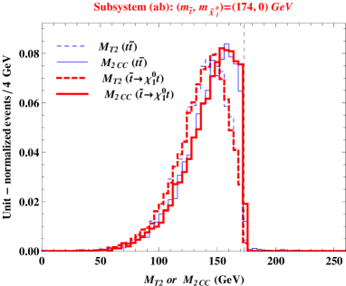
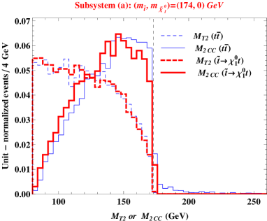
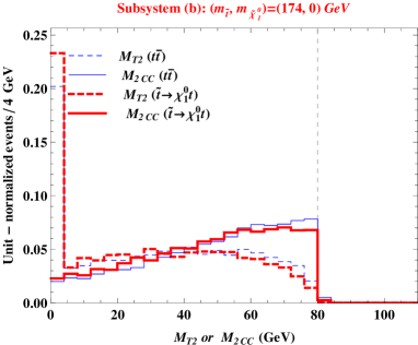
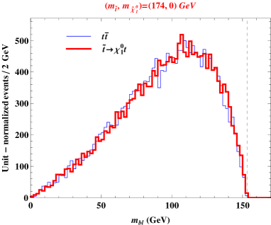
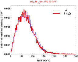
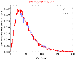
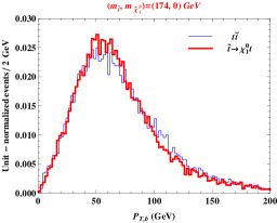
Fig. 16 shows that the $p_{T}$ distributions and the $MET$ distribution are almost identical for signal and background. The invariant mass distributions from Fig. 15 are also very similar; there are slight differences in the shapes due to the top quarks in the signal being more likely to be off-shell, but the kinematic endpoints are the same. Thus, barring a shape-based analysis, there are no obvious cuts which could discriminate signal from background. Therefore, just like study point 4, this would be a very difficult, and most likely impossible, scenario for discovery using these methods. As before, we shall leave this as an open question to be revisited in Sec. 5.

5 $M_{2}$ endpoint study for mixed events

In this section, we shall consider signal events with the mixed event topology of Fig. 2(d). In doing so, we are motivated by two factors:

• In any realistic model, the stop is likely to have several relevant decay modes. (Here we consider the simplest scenario with only the two decay modes from Fig. 1.) Since the stops are pair-produced, the number of signal events in each symmetric channel is proportional to the corresponding branching ratio squared. For mixed events, where the two stops decay differently, the number of signal events benefits from an additional combinatorial factor of 2.

• In the course of our study of the symmetric event topologies from Fig. 2(b) (in Sec. 3) and Fig. 2(c) (in Sec. 4), we determined that there are “blind spots” in the mass parameter space, where the signal resembles the background, and discovery is very challenging. Study points 4 and 6 are examples of such difficult cases. In this section, therefore, we shall investigate the question of whether one can recover some sensitivity by considering mixed events constructed from precisely those two difficult cases. In other words, we consider events with the event topology of Fig. 2(d), where the upper (lower) decay chain corresponds to study point 4 (study point 6). (Study point 4 gives the stop mass ($174$ GeV) and the neutralino mass ($0$ GeV); study point 6 uses the same stop mass, a chargino mass of $150$ GeV and a sneutrino mass of $110$ GeV.) We shall assume that the two stop decays occur with equal branching fractions.

The idea to use mixed stop events was previously discussed in Ref. Graesser:2012qy , which suggested a new variable, “topness”, that quantifies how well an event can be reconstructed under the top background hypothesis. In order to calculate the “topness” of an event, one minimizes the total $\sqrt{s}$ of the event, making the reasonable ansatz that the momentum configuration thus obtained provides a good approximation to the true kinematics of the event Graesser:2012qy ; Konar:2008ei . Our approach is similar to the extent that the on-shell constrained invariant mass variables, like $M_{2CC}$, are also found by minimization, though not of the total $\sqrt{s}$ but of the parent mass in the respective subsystem. By imposing the symmetry constraints (4) and (7), we focus on the one key difference between the signal and background events: the signal event topology is asymmetric while the background event topology is symmetric. We can therefore expect that the constraints (4) and (7) will affect signal and background events differently.

Figure 17: The same as Figs. 11 and 15, comparing distributions of the three $M_{T2}$ subsystem variables and the invariant mass $m_{b\ell}$ for the four types of events in Fig. 2. The mass spectrum corresponds to study points 4 and 6: $m_{\tilde{t}}=174$ GeV, $m_{\tilde{\chi}^{\pm}}=150$ GeV, $m_{\tilde{\nu}}=110$ GeV, and $m_{\tilde{\chi}^{0}}=0$ GeV.

Figure 18: The same as Fig. 17, but for the on-shell constrained variable $M_{2CC}$ in the three possible subsystems $(ab)$, $(a)$, and $(b)$.

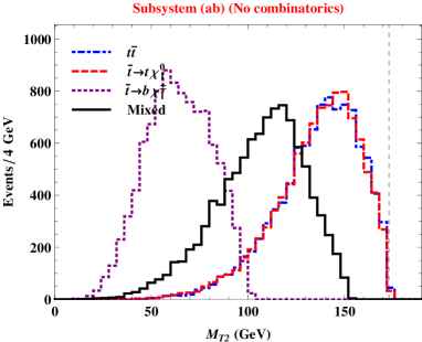
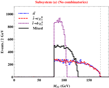
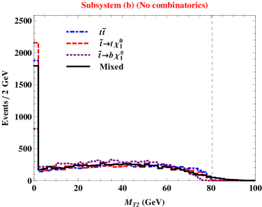
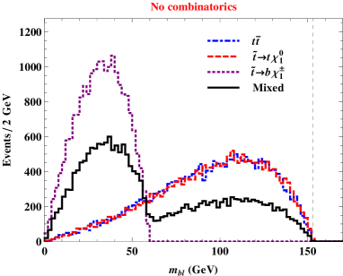
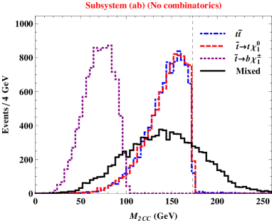
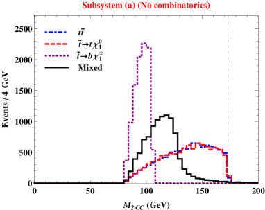
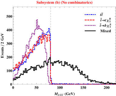
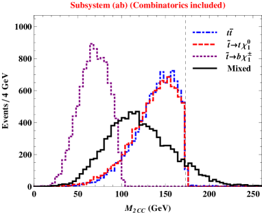
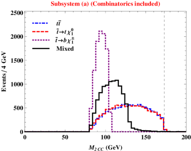
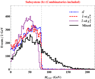
As a point of reference, we begin by showing distributions of variables for which no improvement can be expected in the case of mixed events in Fig. 17. The four variables depicted in the figure are the three subsystem $M_{T2}$ variables and the invariant mass $m_{b\ell}$. All four variables are calculated here using the assignment of the leptons and b-quarks to the correct decay chains. Each panel contains four distributions, one for each event type from Fig. 2: the $t\bar{t}$ background from Fig. 2(a) (blue dot-dashed lines); the symmetric $\tilde{t}\to b\tilde{\chi}^{+}_{1}$ signal events from Fig. 2(b) (magenta dotted lines); the symmetric $\tilde{t}\to t\tilde{\chi}^{0}_{1}$ signal events from Fig. 2(c) (red dashed lines); and the asymmetric signal events from Fig. 2(d) (black solid lines). The vertical black dashed line in each panel marks the location of the upper kinematic endpoint of the $t\bar{t}$ background distribution. We see that for all three types of signal events (symmetric or asymmetric), the respective distributions do not violate the background kinematic endpoints, thus discovery appears to be just as difficult with mixed events as it was with the symmetric events considered earlier in Secs. 3.5 and 4.2. This conclusion is easy to understand; the $M_{T2}$ variable is a variable defined on the transverse plane, where it is impossible to impose a 3+1-dimensional mass constraint like Eq. (4) or (7).

Figure 19: The correlation between the two best performing variables from Fig. 18, for the three types of signal events: pure Topology 1 from Fig. 2(b) (upper left), pure Topology 2 from Fig. 2(c) (upper right), mixed topology from Fig. 2(d) (lower left), and combined total (lower right).

The situation is quite different when we consider distributions of on-shell constrained variables, $M_{2CC}$, for which the constraints of Eqs. (4) or (7) are imposed. As seen in Fig. 18, the signal distributions for mixed events may now exhibit endpoint violation, even when the signal distributions for symmetric events do not. The effect is most pronounced in the case of the subsystem variable $M_{2CC}(b)$; for the subsystem variable $M_{2CC}(ab)$ it is less noticeable, while for $M_{2CC}(a)$ it is absent altogether. Fig. 18 showcases the main result of this section: that with the help of an appropriately chosen on-shell constrained variable (in this case $M_{2CC}(b)$), one can obtain a relatively good separation of signal from background for mixed events. It is worth emphasizing that this separation was achieved for a very unfavorable choice of mass parameters, as the study points 4 and 6 were not observable using events where both decay chains had the same topology.

Figure 20: The same as Fig. 18, but including the effects of combinatorics: for each event, we try both possible assignments of the lepton-$b$pairs, and plot the smaller of the two resulting $M_{2CC}$ values.

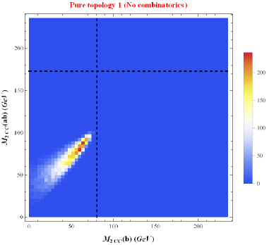
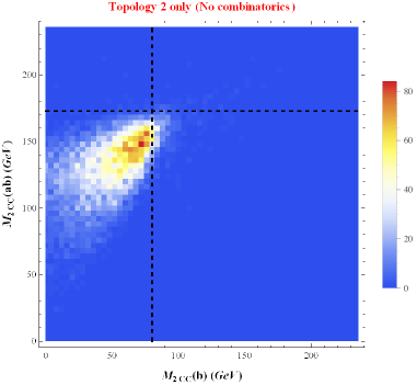
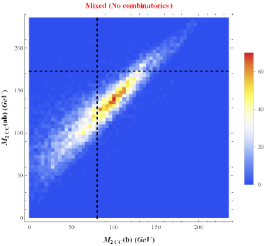
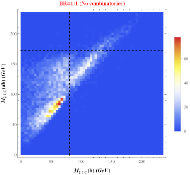
Given that endpoint violation was observed for both $M_{2CC}(b)$ and $M_{2CC}(ab)$, it is worth investigating the possible correlation between those two variables. In Fig. 19 we show two-dimensional plots exhibiting those correlations. We consider separately the three types of signal events: pure Topology 1 from Fig. 2(b) (upper left), pure Topology 2 from Fig. 2(c) (upper right), and the mixed topology from Fig. 2(d) (lower left). Finally, the lower right panel in Fig. 19 shows the result for the full signal sample, with equal branching fractions for Topology 1 and Topology 2. The black dashed lines in Fig. 19 mark the locations of the expected upper kinematic endpoints for background events, following Eqs. (15) and (13). Any events which appear to the right of the vertical black dashed lines and/or above the horizontal black dashed lines in Fig. 19 are expected to be signal-like. In agreement with Fig. 18, we see that for symmetric signal event topologies (the upper two panels in Fig. 19), the signal events are contained within the “background-like” rectangular region adjacent to the origin. On the other hand, for the asymmetric event topology of Fig. 2(d) (the lower left panel), many signal events leak out of the background-like box. The figure also reveals a linear correlation between $M_{2CC}(b)$ and $M_{2CC}(ab)$. Furthermore, the slope is such that if an event violates the background $M_{2CC}(ab)$ endpoint (13), it also necessarily violates the background $M_{2CC}(b)$ endpoint (15), while the reverse is not true. We therefore conclude that the $M_{2CC}(b)$ distribution alone is sufficient in separating signal from background in this scenario with mixed events.

Figure 21: The same as Fig. 19, but including the effects of combinatorics as in Fig. 20.

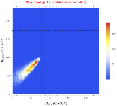
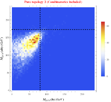
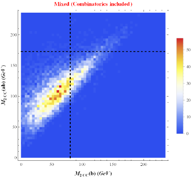
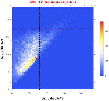
In our discussion so far in this section, we have been ignoring the combinatorial problem arising when we try to pair up the two $b$-jets with the two leptons. Since the $b$-quark charge is not measured, we have two possible pairings, each resulting in a candidate value for the kinematic variable. Since we are interested in upper kinematic endpoints, the simplest solution is to consider both pairings and then pick the one which gives the smaller value for the kinematic variable. This approach has been followed in recreating Figs. 18 and 19 as Figs. 20 and 21, respectively. As expected, this procedure tends to shift all distributions towards lower values, thus the number of signal events which violate the background endpoints is fewer than before; compare, e.g., the $M_{2CC}(b)$ distributions for mixed events in Figs. 18 and 20. Nevertheless, the effect is still present, offering hope that difficult cases like study points 4 and 6 could perhaps best be looked for in such mixed event topologies instead.

6 Results with realistic detector simulation

In the previous three sections we saw that the $M_{T2}$ and $M_{2CC}$ variables allow us to identify signal events as tails which extend beyond the upper kinematic endpoint for background events. However, in a realistic experiment, the background distributions themselves may acquire high tails, for a variety of reasons. This is why it is necessary to test our previous observations, which were made at parton level, with realistic simulation, including the effects of detector resolution, initial and final state radiation, jet reconstruction, cuts, etc. It is clear that our positive conclusions drawn for fortuitous cases of new physics like study point 1 will survive all these complications, therefore in this section we shall only focus on the difficult scenario discussed in Sec. 5, i.e., the mixed events which were a hybrid between the difficult study points 4 from Sec. 3.5 and 6 from Sec. 4.2.

6.1 Event simulation details

As before, the parton-level event generation is done by MadGraph_aMC@NLO Alwall:2014hca , where by default the parton distributions are evaluated by NNPDF23 Ball:2012cx . The relevant output is then piped through Pythia 6.4 Sjostrand:2006za and Delphes3 deFavereau:2013fsa . For both signal and $t\bar{t}$ background, the decays of top quarks are handled by Pythia 6.4, while Topology 1 is explicitly generated by MadGraph_aMC@NLO without any prior cuts. All simulations are performed at leading order for a $pp$ collider of $\sqrt{s}=14$ TeV.

For the signal process, we assume that the branching ratio of Topology 1 relative to Topology 2 is $1:1$. In addition, in Topology 1, the chargino is forced to decay exclusively into a sneutrino (which may further decay invisibly), and a lepton (i.e., electron and muon only). In Topology 2, the stop decays to the lightest neutralino and a top quark, which subsequently decays with the relevant branching ratios predicted in the SM. For our purposes, we only consider the dilepton final state, in which both top quarks decay leptonically. The input top quark mass is set to $173$ GeV, while the $W^{\pm}$ gauge boson mass is $80$ GeV. Jets are reconstructed with the anti-$k_{t}$ algorithm Cacciari:2008gp , using a radius parameter $R=0.5$. The $b$-tagging efficiency is taken to be $70$%, while light quark jets are mis-tagged at the rate of $1$%.

Given the final state $2b+2\ell+E_{T}/\hskip 7.11317pt$, in principle there are several sources of SM background that need to be taken into account. In order to suppress the reducible SM backgrounds, we apply the following pre-selection cuts:

• The event must contain exactly two opposite sign leptons with $p_{T}>10$ GeV and $|\eta|<2.5$ ($|\eta|<2.4$) for electrons (muons).

• In order to reduce background from low mass resonances, in the $ee$ and $\mu\mu$ channels, we demand $m_{ee/\mu\mu}>20$ GeV. Furthermore, to reduce the $Z+$jets background, events with dilepton masses within the $Z$-mass window are vetoed by requiring $|m_{ee/\mu\mu}-m_{Z}|>15$ GeV.

• To further suppress Drell-Yan, for the $ee$ and $\mu\mu$ channels, we apply a missing transverse energy cut of $E_{T}/\hskip 7.11317pt>40$ GeV.

• The event is required to have $\geq 2$ jets with $p_{T}>30$ GeV and $|\eta|<2.4$. It is also required that exactly two of these jets are $b$-tagged.

After these cuts, we are left with $t\bar{t}$ as the dominant (irreducible) background, and this will be the only background process we will consider here. The posterior cuts using $M_{2}$ variables are imposed for events already passing the above set of pre-selection cuts.

6.2 Results for $M_{T2}$ and $M_{2CC}$

We first revisit our results from Sec. 5, this time including the effects of detector simulation and combinatorics. As before, we consider both pairings of the two tagged $b$-jets and the two leptons, and use the smaller of the two resulting values for the kinematic variable under consideration. However, unlike the plots in Sec. 5, here we do not separate the three types of signal events (Topology 1, Topology 2 and mixed), since in the real experiment there is no way to tell which is which.

Figure 22: The same as Fig. 17, but including the effects of combinatorics and detector simulation. The vertical black dashed lines denote the expected $M_{T2}$ endpoints of the $t\bar{t}$ background in each subsystem.

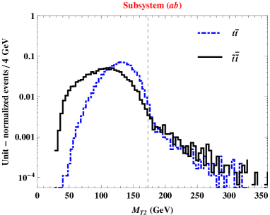
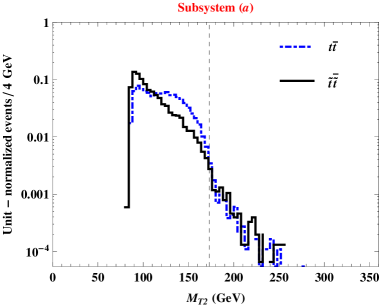
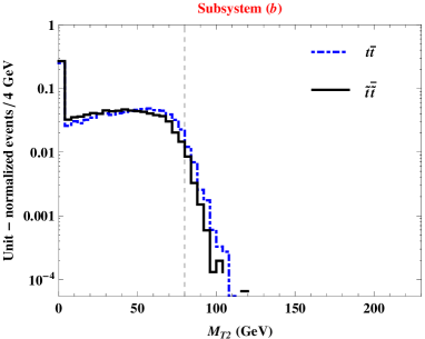
Fig. 22 compares the signal and $t\bar{t}$ background distributions for the three different $M_{T2}$ subsystem variables. As expected from the parton-level results in Sec. 5 (see Fig. 17), the discrimination power in the high tail region is relatively poor, since the signal and the background events obey the same kinematic endpoints.

Figure 23: The same as Fig. 22, but for the corresponding $M_{2CC}$ variables.

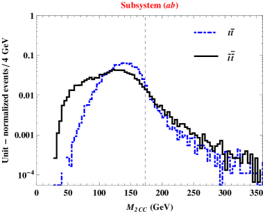
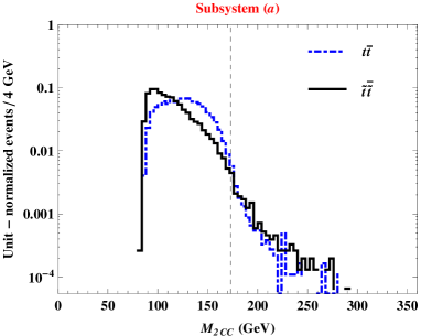
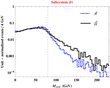
Fig. 23 shows the corresponding $M_{2CC}$ distributions for signal and $t\bar{t}$ background events in the three subsystems. As anticipated from the parton-level result in Figs. 18 and 20, there is a noticeable improvement in the $(b)$ subsystem (for which the visible particle is a lepton) as seen in the lower panel and a slight improvement in the $(ab)$ subsystem as well. Therefore, one would expect that a minimum $M_{2CC}$ cut would be beneficial. The optimal value of the cut would depend on the expected signal cross-section, and on the assumed systematic uncertainty on the background normalization in the high tail region.

A careful comparison of the parton-level results in Figs. 17, 18 and 20 versus the detector-level results in Figs. 22 and 23 reveals that at the detector level the background distributions develop high tails which, unless properly understood, could be confused with a signal. We have checked that in the majority of cases, background events populate the high tail due to imperfect $b$-tagging. A typical event looks as follows: one of the two $b$-jets is either too soft to pass the jet ID cuts, or is not tagged as a $b$-jet. (Recall that the $b$-jet tagging inefficiency is $30$%.) Instead, a gluon from initial state radiation (ISR) forms a hard jet which is subsequently mistagged as a $b$-jet. Thus in computing the $M_{T2}$ and $M_{2CC}$ variables one is using the wrong $b$-jet object, which leads to the endpoint violation. An improvement in the $b$-tagging algorithm, especially one which lowers the mistag rate for ordinary QCD jets, would help alleviate this problem.

6.3 Results for the relative shift from $M_{T2}$ to $M_{2CC}$

In all of our analysis so far, we have relied on the existence of the background kinematic endpoints (13-15) and focused on the high tails above those endpoints. Ideally, this kinematic region should be populated only by signal events, even when one accounts for the two-fold combinatorial ambiguity in pairing the leptons and the $b$-jets. Unfortunately, as we have already seen, this straightforward approach has two drawbacks:

• Presence of high tails in the background distributions. While in theory the background distributions are not supposed to extend beyond their kinematic endpoints, in practice this is not always the case. Such tails were readily observed in Figs. 22 and 23, which were obtained using realistic detector simulation.

• Low signal efficiency. Unless we are dealing with a new physics model with a widely split spectrum (see related discussion in Sec. 3.1), a significant fraction of the signal events will also lie below the background kinematic endpoints, thus by cutting at or near the endpoint, we will be removing a large chunk of signal events as well. This was very evident in the “worst case” scenarios like study points 4 and 6, or the mixed event case discussed in Secs. 5 and 6.2.

These two problems suggest that we should reexamine the region below the background kinematic endpoints and search for a good discriminating variable which would be applicable to that region as well. As in Sec. 5, our goal will be to target signal events with the mixed event topology of Fig. 2(d).

To begin with, recall the main difference between the background events described by Fig. 2(a) and the signal described by Fig. 2(d): the background events are symmetric while the signal events are asymmetric. The on-shell constrained variables $M_{2CX}$, $M_{2XC}$, and $M_{2CC}$ are obtained by applying the additional constraints of Eqs. (4) and (7), which assume that the events are symmetric. Enforcing these constraints leads to the hierarchy (16) which is simply due to the fact that a constrained minimum is larger than an unconstrained minimum. Since the background events are symmetric, the constraints (4) and (7) will be satisfied for the true values of the invisible momenta, and, as long as the global minimum is not too far away (in momentum space), one can expect a relatively mild hierarchy (16). Conversely, for signal events with the mixed event topology, the true values of the invisible momenta in general do not satisfy the constraints (4) and (7). Thus one could expect that the effect of imposing the constraints would be larger, leading to a larger hierarchy (16).

These intuitive considerations suggest that we look at the shift of the on-shell constrained invariant mass variable which is caused by the constraint itself. Keeping in mind the identity $M_{T2}=M_{2XX}$ Cho:2014naa , we can take the usual stransverse mass $M_{T2}$ as our benchmark variable in the absence of any constraints. Then, we can “measure” the effect of the constraints by comparing $M_{T2}$ to $M_{2CC}$, where both (4) and (7) have been applied. This motivates the consideration of a new variable

$$\Delta M(S;\tilde{m})\equiv\sqrt{M^{2}_{2CC}(S;\tilde{m})-M^{2}_{T2}(S;\tilde{m})}.$$ (32)

As indicated in (32), this variable can be computed for any of the three subsystems. We have checked that in our example here, the $(ab)$ subsystem shows the best discrimination between the signal and $t\bar{t}$ background.

Figure 24: Density plots exhibiting the correlations between the variables $\Delta M(ab)$ and $M_{T2}(ab)$ for background events (upper left) and for the three types of signal events: with pure Topology 1 from Fig. 2(b) (upper right), pure Topology 2 from Fig. 2(c) (lower left), and the mixed topology from Fig. 2(d) (lower right).

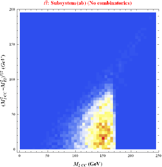
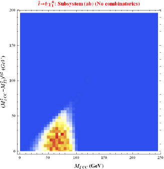
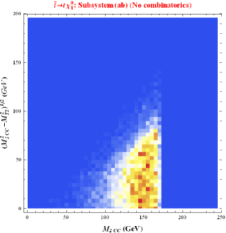
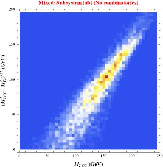
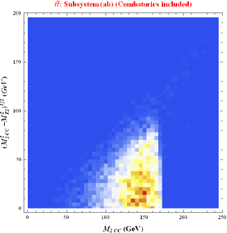
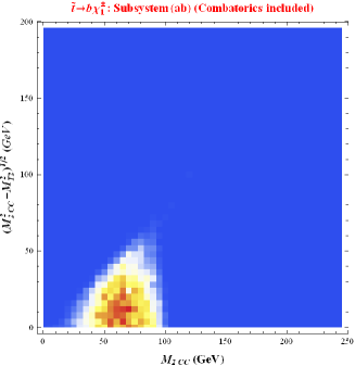
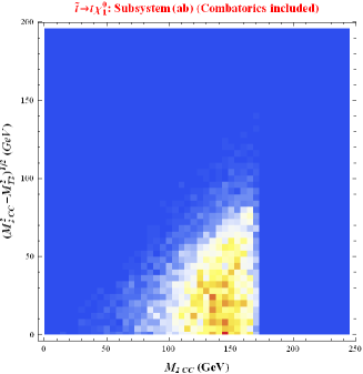
Therefore, in Fig. 24, we contrast the new variable $\Delta M(ab)$ defined in (32) with the variable $M_{2CC}(ab)$ advocated above in Sec. 5. Each panel in Fig. 24 shows a specific type of events at parton level: $t\bar{t}$ background events (upper left panel), signal events with pure Topology 1 from Fig. 2(b) (upper right panel), signal events with pure Topology 2 from Fig. 2(c) (lower left panel), and signal events with mixed topology from Fig. 2(d) (lower right panel). We see that, as already observed in Fig. 18, a certain number of signal events in the mixed channel exceed the background endpoint for $M_{2CC}$. More importantly, the figure also shows that there are many more signal events which do not exceed the background endpoint, yet their value for $\Delta M$ is significantly larger than that for a typical background event. The situation does not change much if we account for the two-fold combinatorial ambiguity, as demonstrated by Fig. 25. We conclude that $\Delta M$ possesses additional discriminating power, and therefore, for an optimal analysis, one should use both $\Delta M$ and $M_{2CC}$ as discriminating variables.

Figure 25: The same as Fig. 24, but including combinatoric effects: each variable $M_{T2}$ and $M_{2CC}$ is separately calculated with the $b$-$\ell$ pairing which gives the lower value for the corresponding variable.

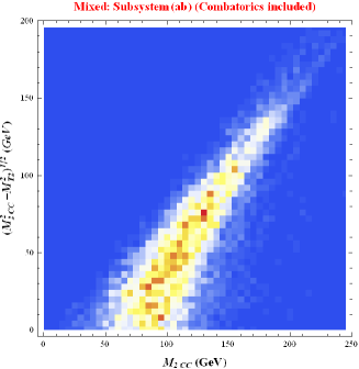
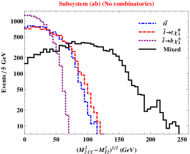
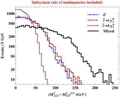
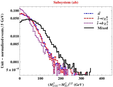
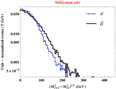
For completeness, we also present results for the $\Delta M$ variable alone. Fig. 26 shows unit-normalized distributions for $\Delta M(ab)$ at the parton level (upper row) and after detector simulation and selection cuts (lower row). The upper left panel is done with perfect assignment for the lepton–$b$-jet pairing, while the upper right panel accounts for the two-fold combinatorial ambiguity as before. The lower right panel shows the observable total signal distribution, which is made up of the individual components identified on the lower left panel. Clearly, the variable $\Delta M(ab)$ performs quite well for signal events with a mixed event topology, and to some extent for signal events with Topology 1. The effect is diluted, but still visible after detector simulation (panels in the lower row).

Figure 26: Unit-normalized distributions of the $\Delta M(ab)$ variable for signal and background events, with the same color coding scheme used in earlier figures. The top row shows parton level results before any selection cuts, while the bottom row includes detector simulation and selection cuts. The upper right (upper left) panel does (does not) account for the two-fold combinatorial ambiguity.

6.4 An alternative variable: the “relative” mass difference

In the previous section, we proposed the variable, $\Delta M$, as a measure of the effect of the constraints (4) and (7). The idea was to look at the change in the value of $M_{2}$ as a result of enforcing these constraints. Let us now look at a different way of capturing the same effect.

Recall that as a result of the minimization involved in calculating the unconstrained $M_{2XX}$ variable, one obtains values for the invisible momenta that minimize the maximal parent particle invariant mass in the specified subsystem. While these are not necessarily the true momenta of the invisible particles in the event, they do provide an useful ansatz and can be used to calculate various $3+1$-dimensional kinematic quantities of interest Cho:2014naa . (See also the MAOS method Cho:2008tj ; Park:2011uz .) In particular, we can compute the masses of the parent particles and the relative particles in the event and test whether the constraints (4) and (7) are satisfied or not. However, there is one technical complication: the function which is being minimized in order to compute $M_{2XX}$, sometimes has a flat direction and does not lead to a unique ansatz for the invisible momenta Cho:2014naa . In order to avoid this problem, here we prefer to use the variable, $M_{CX}$, where the parent constraint (4) is already applied. Thus, we will be comparing the masses of the relative particles instead. In analogy to (32), we therefore define

$$\Delta M_{R}(S;\tilde{m})\equiv\sqrt{|M^{2}_{R_{1}}(S;\tilde{m})-M^{2}_{R_{2}}(S;\tilde{m})|}.$$ (33)

Figure 27: The correlation between the parent mass difference $\Delta M_{R}$ defined in (32) and the relative mass difference $\Delta M$ defined in (33) for background events (left) and signal events with the mixed event topology of Fig. 2(d) (right).

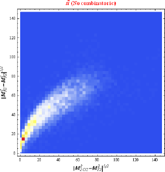
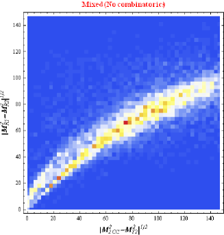
Since they both measure the same effect, namely, the impact of the relative constraint (7), we expect the two variables $\Delta M$ and $\Delta M_{R}$ to be correlated. This is illustrated in Fig. 27, where we compare $\Delta M(ab)$ and $\Delta M_{R}(ab)$ for background events (left panel) and signal events with the mixed event topology of Fig. 2(d) (right panel). The correlation is very evident and suggests that $\Delta M_{R}$ can be used in place of $\Delta M$. The advantage of using $\Delta M_{R}$ is convenience: in order to compute it, one needs to perform a single minimization (that of the variable $M_{2CX}$), while to construct $\Delta M$, one needs to minimize twice: once for $M_{T2}$ (or, equivalently, $M_{2XX}$) and then once for $M_{2CC}$. We have also noticed that our numerical minimization code finds the global minimum of $M_{2CX}$ more reliably than it finds the minimum of the doubly constrained variable $M_{2CC}$.

7 Conclusions and outlook

The search for “top partners,” like top squarks in SUSY, will be a key component of the LHC research program in the next run of the LHC. This is due to several reasons. First, particles which behave like top partners are theoretically well-motivated since they are ubiquitous in models that try to address the hierarchy problem. Second, the experimental limits on third generation partners are generally weaker, leaving room for improvement in the next run. Third, the signatures of top partner production typically resemble those of SM top production, a process which will continue to be under close scrutiny because of the intrinsic interest in the top in its own right.

The main goal of this paper was to tackle certain difficult cases for stop discovery and propose new ideas for improving the experimental sensitivity in the next LHC run. We considered stop signatures which led to an identical final state as the main irreducible top background. Of special interest to us were corners of parameter space which would evade easy detection by normal means, either due to small mass splittings, which lead to soft jets and leptons, or because the new physics signature involves real SM top quarks. Thus we considered the two decay topologies of Fig. 1, which led to the three types of signal events depicted in Fig. 2(b-d).

Given that the signal and background are so similar, discrimination is only possible if we take full advantage of subtle kinematic differences. This is why we focused on the recently proposed class of on-shell constrained variables ($M_{2XX}$, $M_{2CX}$, $M_{2XC}$, and $M_{2CC}$) Mahbubani:2012kx ; Cho:2014naa , which can be suitably defined with the background event topology of Fig. 3 in mind (see Appendix A). These variables have several useful properties which can be used for isolating the signal over the background:

• Existence of upper kinematic endpoints. While the background events obey the bounds (13-15), signal events may violate those bounds, depending on the new physics mass spectrum. Thus, by employing suitable high pass cuts on those variables, one can remove the majority of the background, leaving some fraction of the signal. In Sec. 3.1, we analyzed the relevant mass parameter space and classified the regions where given kinematic endpoints for signal events exceed those for the background. The “easy” regions, where the signal endpoints are significantly above the background endpoints, should be the first targets in the next LHC runs.

• Endpoint violation in the case of the “wrong” event topology. The on-shell kinematic variables were defined with a specific background event topology in mind. If the signal events have a different event topology, either because they are asymmetric (e.g., the mixed event topology of Fig. 2(d)), or because they contain more invisible particles (as in the case of pure Topology 2 in Fig. 2(c)), they may again violate the background endpoints, see Figs. 13 and 18. For concreteness, in this paper we only considered the two specific event topologies from Fig. 1, but in realistic models, there exist other well-motivated event topologies which would lead to the same final state. (A couple of such examples are shown in Fig. 28.) The multitude of possible stop decay modes increases the likelihood that the signal will include asymmetric events, which may manifest themselves through violations of the expected background endpoints.

  

  Figure 28: Two other possible decay topologies leading to the same final state as in Fig. 1.

• The existence of the hierarchy (16) between the various $M_{2\sqcup\sqcup}$ variables. We showed that the hierarchy is relatively mild in the case of symmetric events like the $t\bar{t}$ background and gets stronger as the events become more asymmetric (as in the mixed topology of Fig. 2(d)). This observation allows us to also target signal events which are below the background kinematic endpoints. We believe that the related variables $\Delta M$ and $\Delta M_{R}$ defined in (32) and (33) respectively, will be a useful addition to the experimenter’s arsenal of tools for new physics searches in missing energy events.

In spite of the advances proposed here, these searches remain extremely challenging. Detector effects, jet combinatorics issues due to ISR and FSR, and $b$-jet misidentification contribute to the degradation of the parton level significance. Nevertheless, we believe that the techniques presented here will prove useful in searches for top partners at the LHC.

In this paper, we have employed a simplified model approach as shown in Fig. 2 in order to best make contact with experimental efforts. Of course, when interpreting such simplified model experimental limits or discoveries in terms of some complete theory, one must compute both signal Beenakker:1997ut ; Beenakker:2010nq ; Beenakker:2011fu and background Cacciari:2011hy ; Czakon:2011xx ; Czakon:2012zr ; Czakon:2012pz production cross-sections and the relevant branching ratios Djouadi:2006bz to a high degree of precision.

The on-shell constrained variables are suitable generalizations of the stransverse mass variable, $M_{T2}$, which is being used extensively in experimental searches, and for which several public codes exist. In contrast, there is no public code which allows the computation of the $M_{2}$ variables. We are developing such a code for public release in the near future to facilitate the wider use of $M_{2}$ variables Cho:2015laa .

Appendix A The complete set of $M_{2}$ variables for the $t\bar{t}$ event topology

In this appendix, we collect the specific definitions of the fifteen $M_{2}$ variables used in this paper. We consider the three subsystems in Fig. 3 as applied to the $t\bar{t}$ background events of Fig. 2(a). We write the equations in terms of the measured 4-momenta of the $b$ and $\bar{b}$ quarks, $p_{b}$ and $p_{\bar{b}}$, and the measured 4-momenta of the lepton and antilepton, $p_{\ell^{-}}$ and $p_{\ell^{+}}$. The invisible neutrino 4-momenta will be denoted by $q_{1}$ and $q_{2}$, where we take “1” to refer to the decay chain initiated by a top quark and “2” to refer to the decay chain initiated by an anti-top. In each subsystem, the test mass $\tilde{m}$ is taken to be the corresponding true daughter mass.

In the $(ab)$ subsystem the daughter particles are the two neutrinos, with mass $\tilde{m}=0$. The definitions (8-12) imply

$$M_{2CC}^{2}(ab;\tilde{m}=0) \equiv \min_{\begin{subarray}{c}\vec{q}_{1},\vec{q}_{2}\\ q_{1}^{2}=q_{2}^{2}=\tilde{m}^{2}=0\\ \vec{q}_{1T}+\vec{q}_{2T}={\;/\!\!\!\!\vec{P}_{T}}\\ (p_{b}+p_{\ell^{+}}+q_{1})^{2}=(p_{\bar{b}}+p_{\ell^{-}}+q_{2})^{2}\\ (p_{\ell^{+}}+q_{1})^{2}=(p_{\ell^{-}}+q_{2})^{2}\end{subarray}}\left\{(p_{b}+p_{\ell^{+}}+q_{1})^{2}\right\},$$ (34)

$$M_{2CX}^{2}(ab;\tilde{m}=0) \equiv \min_{\begin{subarray}{c}\vec{q}_{1},\vec{q}_{2}\\ q_{1}^{2}=q_{2}^{2}=\tilde{m}^{2}=0\\ \vec{q}_{1T}+\vec{q}_{2T}={\;/\!\!\!\!\vec{P}_{T}}\\ (p_{b}+p_{\ell^{+}}+q_{1})^{2}=(p_{\bar{b}}+p_{\ell^{-}}+q_{2})^{2}\end{subarray}}\left\{(p_{b}+p_{\ell^{+}}+q_{1})^{2}\right\},$$ (35)

$$M_{2XC}^{2}(ab;\tilde{m}=0) \equiv \!\!\!\!\!\!\!\!\!\min_{\begin{subarray}{c}\vec{q}_{1},\vec{q}_{2}\\ q_{1}^{2}=q_{2}^{2}=\tilde{m}^{2}=0\\ \vec{q}_{1T}+\vec{q}_{2T}={\;/\!\!\!\!\vec{P}_{T}}\\ (p_{\ell^{+}}+q_{1})^{2}=(p_{\ell^{-}}+q_{2})^{2}\end{subarray}}\!\!\!\!\!\!\!\!\!\left\{\max\left[(p_{b}+p_{\ell^{+}}+q_{1})^{2}\;,(p_{\bar{b}}+p_{\ell^{-}}+q_{2})^{2}\right]\right\},~{}~{}~{}~{}$$ (36)

$$M_{2XX}^{2}(ab;\tilde{m}=0) \equiv \!\!\!\!\!\min_{\begin{subarray}{c}\vec{q}_{1},\vec{q}_{2}\\ q_{1}^{2}=q_{2}^{2}=\tilde{m}^{2}=0\\ \vec{q}_{1T}+\vec{q}_{2T}={\;/\!\!\!\!\vec{P}_{T}}\end{subarray}}\!\!\!\!\!\left\{\max\left[(p_{b}+p_{\ell^{+}}+q_{1})^{2}\;,(p_{\bar{b}}+p_{\ell^{-}}+q_{2})^{2}\right]\right\},$$ (37)

$$M_{T2}^{2}(ab;\tilde{m}=0) \equiv \!\!\!\!\!\!\!\min_{\begin{subarray}{c}\vec{q}_{1T},\vec{q}_{2T}\\ \vec{q}_{1T}+\vec{q}_{2T}={\;/\!\!\!\!\vec{P}_{T}}\end{subarray}}\!\!\!\!\!\!\!\left\{\max\left[M^{2}_{Tt}(\vec{q}_{1T},\tilde{m}=0),\;M^{2}_{T\bar{t}}(\vec{q}_{2T},\tilde{m}=0)\right]\right\}.$$ (38)

In the last equation $M_{Tt}$ ($M_{T\bar{t}}$) is the transverse mass of the hypothesized top quark (anti-top quark):

$$M^{2}_{Tt}(\vec{q}_{1T},\tilde{m}) \equiv (E_{Tb}+E_{T\ell^{+}}+E_{T1})^{2}-(\vec{p}_{Tb}+\vec{p}_{T\ell^{+}}+\vec{q}_{1T})^{2},$$ (39)

$$M^{2}_{T\bar{t}}(\vec{q}_{2T},\tilde{m}) \equiv (E_{T\bar{b}}+E_{T\ell^{-}}+E_{T2})^{2}-(\vec{p}_{T\bar{b}}+\vec{p}_{T\ell^{-}}+\vec{q}_{2T})^{2},$$ (40)

with the transverse energies defined as usual, e.g. $E_{Ti}=\sqrt{\tilde{m}^{2}+\vec{q}_{Ti}^{\,2}}$.

In the $(b)$ subsystem the daughter particles are again the massless neutrinos, but this time we minimize the masses of the hypothesized $W^{\pm}$ particles:

$$M_{2CC}^{2}(b;\tilde{m}=0) \equiv \min_{\begin{subarray}{c}\vec{q}_{1},\vec{q}_{2}\\ q_{1}^{2}=q_{2}^{2}=\tilde{m}^{2}=0\\ \vec{q}_{1T}+\vec{q}_{2T}={\;/\!\!\!\!\vec{P}_{T}}\\ (p_{b}+p_{\ell^{+}}+q_{1})^{2}=(p_{\bar{b}}+p_{\ell^{-}}+q_{2})^{2}\\ (p_{\ell^{+}}+q_{1})^{2}=(p_{\ell^{-}}+q_{2})^{2}\end{subarray}}\left\{(p_{\ell^{+}}+q_{1})^{2}\right\},$$ (41)

$$M_{2CX}^{2}(b;\tilde{m}=0) \equiv \min_{\begin{subarray}{c}\vec{q}_{1},\vec{q}_{2}\\ q_{1}^{2}=q_{2}^{2}=\tilde{m}^{2}=0\\ \vec{q}_{1T}+\vec{q}_{2T}={\;/\!\!\!\!\vec{P}_{T}}\\ (p_{\ell^{+}}+q_{1})^{2}=(p_{\ell^{-}}+q_{2})^{2}\end{subarray}}\left\{(p_{\ell^{+}}+q_{1})^{2}\right\},$$ (42)

$$M_{2XC}^{2}(b;\tilde{m}=0) \equiv \!\!\!\!\!\!\!\!\!\min_{\begin{subarray}{c}\vec{q}_{1},\vec{q}_{2}\\ q_{1}^{2}=q_{2}^{2}=\tilde{m}^{2}=0\\ \vec{q}_{1T}+\vec{q}_{2T}={\;/\!\!\!\!\vec{P}_{T}}\\ (p_{b}+p_{\ell^{+}}+q_{1})^{2}=(p_{\bar{b}}+p_{\ell^{-}}+q_{2})^{2}\end{subarray}}\!\!\!\!\!\!\!\!\!\left\{\max\left[(p_{\ell^{+}}+q_{1})^{2}\;,(p_{\ell^{-}}+q_{2})^{2}\right]\right\},~{}~{}~{}~{}$$ (43)

$$M_{2XX}^{2}(b;\tilde{m}=0) \equiv \min_{\begin{subarray}{c}\vec{q}_{1},\vec{q}_{2}\\ q_{1}^{2}=q_{2}^{2}=\tilde{m}^{2}=0\\ \vec{q}_{1T}+\vec{q}_{2T}={\;/\!\!\!\!\vec{P}_{T}}\end{subarray}}\left\{\max\left[(p_{\ell^{+}}+q_{1})^{2}\;,(p_{\ell^{-}}+q_{2})^{2}\right]\right\},$$ (44)

$$M_{T2}^{2}(b;\tilde{m}=0) \equiv \!\!\!\!\!\!\!\!\!\min_{\begin{subarray}{c}\vec{q}_{1T},\vec{q}_{2T}\\ \vec{q}_{1T}+\vec{q}_{2T}={\;/\!\!\!\!\vec{P}_{T}}\end{subarray}}\!\!\!\!\!\!\!\!\!\left\{\max\left[M^{2}_{TW^{+}}(\vec{q}_{1T},\tilde{m}=0),\;M^{2}_{TW^{-}}(\vec{q}_{2T},\tilde{m}=0)\right]\right\},~{}~{}~{}~{}$$ (45)

with

$$M^{2}_{TW^{+}}(\vec{q}_{1T},\tilde{m}) \equiv (E_{T\ell^{+}}+E_{T1})^{2}-(\vec{p}_{T\ell^{+}}+\vec{q}_{1T})^{2},$$ (46)

$$M^{2}_{TW^{-}}(\vec{q}_{2T},\tilde{m}) \equiv (E_{T\ell^{-}}+E_{T2})^{2}-(\vec{p}_{T\ell^{-}}+\vec{q}_{2T})^{2}.$$ (47)

Finally, consider the $(a)$ subsystem, in which the the parents are the top quarks, while the daughters are the $W^{\pm}$ bosons, with masses $\tilde{m}=m_{W}$. Denoting now the 4-momenta of the two hypothesized $W^{\pm}$ bosons with $q_{W^{+}}$ and $q_{W^{-}}$, we have

$$M_{2CC}^{2}(a;\tilde{m}=m_{W}) \equiv \min_{\begin{subarray}{c}\vec{q}_{W^{+}},\vec{q}_{W^{-}}\\ q_{W^{+}}^{2}=q_{W^{-}}^{2}=\tilde{m}^{2}=m_{W}^{2}\\ \vec{q}_{TW^{+}}+\vec{q}_{TW^{-}}={\;/\!\!\!\!\vec{P}_{T}}+\vec{p}_{T\ell^{+}}+\vec{p}_{T\ell^{-}}\\ (p_{b}+q_{W^{+}})^{2}=(p_{\bar{b}}+q_{W^{-}})^{2}\\ (q_{W^{+}}-p_{\ell^{+}})^{2}=(q_{W^{-}}-p_{\ell^{-}})^{2}\end{subarray}}\left\{(p_{b}+q_{W^{+}})^{2}\right\},$$ (48)

$$M_{2CX}^{2}(a;\tilde{m}=m_{W}) \equiv \min_{\begin{subarray}{c}\vec{q}_{W^{+}},\vec{q}_{W^{-}}\\ q_{W^{+}}^{2}=q_{W^{-}}^{2}=\tilde{m}^{2}=m_{W}^{2}\\ \vec{q}_{TW^{+}}+\vec{q}_{TW^{-}}={\;/\!\!\!\!\vec{P}_{T}}+\vec{p}_{T\ell^{+}}+\vec{p}_{T\ell^{-}}\\ (p_{b}+q_{W^{+}})^{2}=(p_{\bar{b}}+q_{W^{-}})^{2}\end{subarray}}\left\{(p_{b}+q_{W^{+}})^{2}\right\},$$ (49)

$$M_{2XC}^{2}(a;\tilde{m}=m_{W}) \equiv \!\!\!\!\!\!\!\!\!\!\!\!\min_{\begin{subarray}{c}\vec{q}_{W^{+}},\vec{q}_{W^{-}}\\ q_{W^{+}}^{2}=q_{W^{-}}^{2}=\tilde{m}^{2}=m_{W}^{2}\\ \vec{q}_{TW^{+}}+\vec{q}_{TW^{-}}={\;/\!\!\!\!\vec{P}_{T}}+\vec{p}_{T\ell^{+}}+\vec{p}_{T\ell^{-}}\\ (q_{W^{+}}-p_{\ell^{+}})^{2}=(q_{W^{-}}-p_{\ell^{-}})^{2}\end{subarray}}\!\!\!\!\!\!\!\!\!\left\{\max\left[(p_{b}+q_{W^{+}})^{2}\;,(p_{\bar{b}}+q_{W^{-}})^{2}\right]\right\},~{}~{}~{}~{}$$ (50)

$$M_{2XX}^{2}(a;\tilde{m}=m_{W}) \equiv \!\!\!\!\!\!\!\!\!\!\!\!\min_{\begin{subarray}{c}\vec{q}_{W^{+}},\vec{q}_{W^{-}}\\ q_{W^{+}}^{2}=q_{W^{-}}^{2}=\tilde{m}^{2}=m_{W}^{2}\\ \vec{q}_{TW^{+}}+\vec{q}_{TW^{-}}={\;/\!\!\!\!\vec{P}_{T}}+\vec{p}_{T\ell^{+}}+\vec{p}_{T\ell^{-}}\end{subarray}}\!\!\!\!\!\!\!\!\!\left\{\max\left[(p_{b}+q_{W^{+}})^{2}\;,(p_{\bar{b}}+q_{W^{-}})^{2}\right]\right\},$$ (51)

$$M_{T2}^{2}(a;\tilde{m}=m_{W}) \equiv \!\!\!\!\!\!\!\!\!\!\!\!\!\!\!\!\!\!\!\!\!\!\min_{\begin{subarray}{c}\vec{q}_{W^{+}},\vec{q}_{W^{-}}\\ \vec{q}_{TW^{+}}+\vec{q}_{TW^{-}}={\;/\!\!\!\!\vec{P}_{T}}+\vec{p}_{T\ell^{+}}+\vec{p}_{T\ell^{-}}\end{subarray}}\!\!\!\!\!\!\!\!\!\!\!\!\!\!\!\!\!\!\!\!\!\!\!\!\!\!\left\{\max\left[M^{2}_{Tt}(\vec{q}_{TW^{+}},m_{W}),\;M^{2}_{T\bar{t}}(\vec{q}_{TW^{-}},m_{W})\right]\right\},$$ (52)

where now the top quark transverse masses (39-40) are rewritten in terms of the $W^{\pm}$ boson momenta, $q_{W^{+}}$ and $q_{W^{-}}$, as

$$M^{2}_{Tt}(\vec{q}_{TW^{+}},\tilde{m}=m_{W}) \equiv (E_{Tb}+E_{TW^{+}})^{2}-(\vec{p}_{Tb}+\vec{q}_{TW^{+}})^{2},$$ (53)

$$M^{2}_{T\bar{t}}(\vec{q}_{TW^{-}},\tilde{m}=m_{W}) \equiv (E_{T\bar{b}}+E_{TW^{-}})^{2}-(\vec{p}_{T\bar{b}}+\vec{q}_{TW^{-}})^{2},$$ (54)

with $E_{TW^{\pm}}=\sqrt{m_{W}^{2}+\vec{q}_{TW^{\pm}}^{\,2}}$.