Many-body localization edge in the random-field Heisenberg chain

Abstract

We present a large scale exact diagonalization study of the one dimensional spin $1/2$ Heisenberg model in a random magnetic field. In order to access properties at varying energy densities across the entire spectrum for system sizes up to $L=22$ spins, we use a spectral transformation which can be applied in a massively parallel fashion. Our results allow for an energy-resolved interpretation of the many body localization transition including the existence of an extensive many-body mobility edge. The ergodic phase is well characterized by Gaussian orthogonal ensemble statistics, volume-law entanglement, and a full delocalization in the Hilbert space. Conversely, the localized regime displays Poisson statistics, area-law entanglement and non ergodicity in the Hilbert space where a true localization never occurs. We perform finite size scaling to extract the critical edge and exponent of the localization length divergence.

The interplay of disorder and interactions in quantum systems can lead to several intriguing phenomena, amongst which the so-called many-body localization has attracted a huge interest in recent years. Following precursors works Fleishman and Anderson (1980); Altshuler et al. (1997); Jacquod and Shepelyansky (1997); Georgeot and Shepelyansky (1998), perturbative calculations Gornyi et al. (2005); Basko et al. (2006) have established that the celebrated Anderson localization Anderson (1958) can survive interactions, and that for large enough disorder, many-body eigenstates can also “localize” (in a sense to be precised later) and form a new phase of matter commonly referred to as the many-body localized (MBL) phase.

The enormous boost of interest for this topic over the last years can probably be ascribed to the fact that the MBL phase challenges the very foundations of quantum statistical physics, leading to striking theoretical and experimental consequences Nandkishore and Huse ; Altman and Vosk . Several key features of the MBL phase can be highlighted as follows. It is non-ergodic, and breaks the eigenstate thermalization hypothesis (ETH) Deutsch (1991); Srednicki (1994); Rigol et al. (2008): a closed system in the MBL phase does not thermalize solely following its own dynamics. The possible presence of a many-body mobility edge (at a finite energy density in the spectrum) indicates that conductivity should vanish in a finite temperature range in a MBL system Gornyi et al. (2005); Basko et al. (2006). Coupling to an external bath will eventually destroy the properties of the MBL phase, but recent arguments show that it can survive and be detected using spectral signatures for weak bath-coupling Nandkishore et al. (2014). This leads to the suggestion that the MBL phase can be characterized experimentally, using e.g. controlled echo experiments on reasonably well-isolated systems with dipolar interactions Serbyn et al. (2014); Kwasigroch and Cooper (2014); Yao et al. ; Vasseur et al. . Another appealing aspect (with experimental consequences for self-correcting memories) is that MBL systems can sustain long-range, possibly topological, order in situations where equilibrated systems would not Huse et al. (2013); Bahri et al. ; Chandran et al. (2014a); Bauer and Nayak (2013); Vosk and Altman (2014). Finally, a striking phenomenological approach Huse et al. (2014) pinpoints that the MBL phase shares properties with integrable systems, with extensive local integrals of motion Serbyn et al. (2013); Ros et al. ; Chandran et al. (2014b), and that MBL eigenstates sustain low (area law) entanglement. This is in contrast with eigenstates at finite energy density in a generic equilibrated system, which have a large amount (volume law) of entanglement and which are believed to be well described within a random matrix theory approach.

Figure 1: Disorder ($h$) — Energy density ($\epsilon$) phase diagram of the disordered Heisenberg chain Eq. (1). The ergodic phase (dark region with a participation entropy volume law coefficient $a_{1}\simeq 1$) is separated from the localized regime (bright region with $a_{1}\ll 1$). Various symbols (see legend) show the energy-resolved MBL transition points extracted from finite size scaling performed over system sizes $L\in\{14,15,16,17,18,19,20,22\}$. Red squares correspond to a visual estimate of the boundary between volume and area law scaling of entanglement entropy $S_{E}$.

Going beyond perturbative approaches, direct numerical simulations of disordered quantum interacting systems provide a powerful framework to test MBL features in a variety of systems Oganesyan and Huse (2007); Pal and Huse (2010); Žnidarič et al. (2008); Canovi et al. (2011); Cuevas et al. (2012); Bauer and Nayak (2013); Serbyn et al. (2014); Kjäll et al. (2014); De Luca and Scardicchio (2013); Iyer et al. (2013); Pekker et al. (2014); Johri et al. ; Bardarson et al. (2012); Andraschko et al. (2014); Laumann et al. (2014); Vasseur et al. ; Hickey et al. ; Nanduri et al. (2014); Bar Lev and Reichman (2014). The MBL transition dealing with eigenstates at high(er) energy, ground-state methods are not well adapted. Most numerical studies use full exact diagonalization (ED) to obtain all eigenstates and energies and are limited to rather small Hilbert space sizes $\dim{\cal H}\sim 10^{4}$ .

In this Letter, we present an extensive numerical study of the periodic $S=\frac{1}{2}$ Heisenberg chain in a random magnetic field, governed by the Hamiltonian

$$H=\sum_{i\in[1,L]}{\bf S}_{i}\cdot{\bf S}_{i+1}-h_{i}S_{i}^{z},$$ (1)

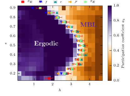
with $h_{i}$ drawn from a uniform distribution $[-h,h]$ (total magnetization $S^{z}$ is conserved). Model (1) has been used Pal and Huse (2010); Bauer and Nayak (2013); De Luca and Scardicchio (2013); Nanduri et al. (2014) as a prototype for the MBL transition in the “infinite-temperature” limit, where the full many-body spectrum (or a large fraction thereof) is considered for systems of maximum size $L\approx 16$. In this work, we instead use a shift-inverse ED approach and are able to reach eigenstates at arbitrary energy density for systems up to $L=22$ with very large Hilbert spaces ($\dim{{\cal H}_{L=22}}=705\,432$ in the $S^{z}=0$ sector). Our simulations unambiguously reveal the existence of an extensive many-body localization edge: the resulting phase diagram (disorder strength $h$ vs. energy density $\epsilon$, Fig. 1) is built on a careful finite size scaling analysis of numerous energy-resolved estimates. In particular the transition is captured using, e.g. spectral statistical correlations between nearby eigenstates, volume vs. area law of entanglement entropies and bipartite fluctuations, spin relaxation, localization properties in the Hilbert space, which all roughly agree within error bars. We also perform a scaling analysis close to the MBL transition.

Characterization of ergodic and localized regimes— Before presenting our numerics, we summarize the main differences between ergodic and localized phases, and the observables used to quantify them.

(i) Level statistics and eigenvectors similarity. A popular way to differentiate extended and localized regimes relies on studying spectral statistics using tools from random matrix theory Mehta (1991). In the ergodic regime, the statistical distribution of level spacings follows Wigner’s surmise of the Gaussian orthogonal ensemble (GOE), while a Poisson distribution is expected for localized states. It is convenient Oganesyan and Huse (2007) to consider the ratio of consecutive level spacings $r^{(n)}={\rm{min}}(\delta^{(n)},\delta^{(n+1)})/{\rm{max}}(\delta^{(n)},\delta^{(n+1)})$ with $\delta^{(n)}=E_{n}-E_{n-1}$ at a given eigen-energy $E_{n}$ to discriminate between the two phases, as its disorder average changes from ${{r}}_{\rm GOE}=0.5307(1)$ Atas et al. (2013) to ${{r}}_{\rm Poisson}=2\ln 2-1\simeq 0.3863$. This has been used in several works Oganesyan and Huse (2007); Pal and Huse (2010); Cuevas et al. (2012); Johri et al. ; Laumann et al. (2014); Bauer and Nayak (2013), averaging over a large part of the spectrum. Here, we compute ${{r}}$ in an energy-resolved way in order to locate the MBL edge (Fig. 2).

Quite interestingly, the GOE–Poisson transition can also be captured by correlations between nearby eigenstates. We expect eigenfunctions to be “similar” (“different”) in the ergodic (localized) regime. We quantify the degree of correlation by the Kullback-Leibler divergence (KLd) Kullback and Leibler (1951), defined by ${\rm KL}=\sum_{i=1}^{\dim{\cal H}}p_{i}\ln(p_{i}/q_{i})$, where $p_{i}=|\langle i|n\rangle|^{2}$ and $q_{i}=|\langle i|n^{\prime}\rangle|^{2}$ are the moduli squared of the wave functions coefficients of 2 nearby eigenstates $|n\rangle,|n^{\prime}\rangle$ expressed in the computational basis $\{|i\rangle\}$ (here $\{S^{z}\}$). The KLd displays different behavior in the two phases (Fig. 2): we find ${\rm{KL}}_{\rm GOE}=2$ , and ${\rm{KL}}_{\rm Poisson}\sim\ln(\dim{\cal H})$.

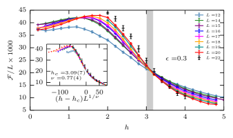
(ii) Entanglement entropy (EE). Beyond level statistics, EE provides a quantitative tool to characterize how information is spread from one part of the system to an other Nandkishore and Huse . In the ergodic regime satisfying the ETH, the reduced density matrix $\rho_{A}$ of a typical eigenstate is expected to be thermal, yielding a volume-law scaling (with the subsystem $A$ size) for the entanglement entropy $S^{E}=-{\rm Tr}\rho_{A}\ln\rho_{A}$. Conversely, localized eigenstates display a much smaller entanglement, expected to cross-over towards an area-law scaling Nandkishore and Huse ; Bauer and Nayak (2013) when the subsystem size exceeds the localization length. These different scalings of $S^{E}$ allow to distinguish both regimes (Fig. 3). In the same spirit, we expect bipartite fluctuations of the subsystem magnetization $S^{z}_{A}$ Song et al. (2012) $\mathcal{F}=\langle\left(S^{z}_{A}\right)^{2}\rangle-\langle S^{z}_{A}\rangle^{2}$ to exhibit similar scaling (Fig. 4).

(iii) Hilbert space localization. Another characterization of MBL relies on inverse participation ratios and associated participation entropies (PE), traditionally used in the context of single particle localization Bell (1972); Wegner (1980); Rodriguez et al. (2011) and recently for many-body physics Luitz et al. (2014a, b). Here the localization is studied in the Hilbert space (of dimension $\dim{\cal H}$) of spin configurations via the disorder average PEs ${S^{\text{P}}_{q}}$, defined for any eigenstate $|n\rangle$ represented in the $\{S^{z}\}$ basis by $S^{\text{P}}_{q}(|n\rangle)=\frac{1}{1-q}\ln\sum_{i}p_{i}^{q}$ [$S^{\text{P}}_{1}(|n\rangle)=-\sum_{i}p_{i}\ln p_{i}$]. We generically find eigenstates to be delocalized in both regimes with qualitatively different features. In the ergodic regime, we obtain a leading scaling $S^{\rm P}_{q}=a_{q}\ln({\dim{\cal H}})$ with $a_{q}\approx 1$ $\forall q$ (see color coding of $a_{1}$ in Fig. 1). In the localized phase, PE also grows with system size (Fig. 5), but much slower with $a_{q}\ll 1$, or $a_{q}=0$ within error bars and a slow log divergence $S^{\rm P}_{q}=l_{q}\ln(\ln{\dim{\cal H}})$, indicating a non-trivial multi-fractal behavior.

Numerical method — The complete diagonalization of the non-translation invariant Hamiltonian Eq. (1) is out of reach for system sizes $L\gtrsim 18$ spins. Therefore, we use an approach successful for the Anderson localization problem (see e.g. Ref. Rodriguez et al., 2011) and restrict ourselves to certain energy slices in the spectrum by using a shift-invert spectral transformation $(\mathbf{H}-E\mathbf{1})^{-1}$. In the transformed problem, it is easy to apply Krylov space methods Hernandez et al. (2005) to compute the eigenpairs closest to the shift energy $E$.

For each disorder realization, we first calculate the extremal eigenenergies $E_{0}$ and $E_{\text{max}}$ used to define the normalized energy target $\epsilon=(E-E_{\text{max}})/(E_{0}-E_{\text{max}})$ (we considered the $S^{z}=0$ sector of even-sized $L=12,14,16,18,20,22$ and $S^{z}=1$ sector of $L=15,17,19$). The shift-invert method, based on a massively parallel $LU$ decomposition Amestoy et al. (2001, 2006), is then used to calculate at least 50 eigenpairs with energy densities closest to the targets $\epsilon=\{0.05,0.1,\dots 0.95\}$. Note that this is a much more demanding computational task than for the Anderson problem, as the number of off-diagonal elements of $H$ scales with $L$. We use at least 1000 disorder realizations for each $L$ (except for $L=22$ where we accumulated between 50 and 250 samples). For each $\epsilon$, observables are calculated from the corresponding eigenvectors and averaged over target packets and disorder realizations for each value of the disorder strength $h$. As eigenvectors of the same disorder realization are correlated, we found it crucial Rodriguez et al. (2011) to bin quantities over all eigenstates of the same realization, and then compute the standard error over these bin averages, in order not to underestimate error bars. Investigating numerous quantities allows to check the consistency of our analysis and conclusions.

Figure 2: Adjacent gap ratio (top) and Kullback Leibler divergence (bottom) as a function of disorder strength in the spectrum center $\epsilon=0.5$. Insets: (top) data collapse used to extract the critical disorder strength $h_{c}$ and exponent $\nu$. The $h$ axis is transformed by $(h-h_{c})L^{1/\nu}$, (bottom) distribution of KLd in both phases.

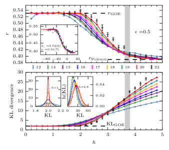
Results and finite size scaling analysis— We discuss the transition between GOE and Poisson statistics, first using the consecutive gap ratio ${\overline{r}}$, shown in Fig. 2 (top) for $\epsilon=0.5$. When varying the disorder strength $h$, we clearly see a crossing around $h_{c}\sim 3.7$ between the two limiting values. This crossing can be analyzed using a scaling form $g[L^{1/\nu}(h-h_{c})]$ which allows a collapse of the data onto a single universal curve (see inset), yielding $h_{c}=3.72(6)$ and $\nu=0.91(7)$ (see details of fitting procedure and error bars estimates in Sup. Mat.).

The above defined KLd, computed for two eigenstates randomly chosen at the same energy target $\epsilon$ and averaged over disordered samples, also displays a crossing between the two limit scalings ${\rm{KL}}_{\rm GOE}=2$ and ${\rm{KL}}_{\rm Poisson}\sim\ln(\dim{\cal H})$ (Fig. 2 bottom). A data collapse is very difficult to achieve for KL due to a large drift of the crossing points. Nevertheless, the distributions of KL plotted in insets, display markedly different features. The perfect gaussian distribution in the ergodic phase (at $h=1$) around the GOE mean value of 2 with a variance decreasing with $L$ provides strong evidence that the statistical behavior of the eigenstates is well described by GOE, extending its applicability beyond simple level statistics. In the MBL regime ($h=4.8$), the behavior is completely different as variance and mean both increase with $L$.

Figure 3: Entanglement entropy per site $S^{\text{E}}/L$ and its variance $\sigma_{E}$, as a function of system size $L$ for different disorder strengths in the middle of the spectrum (left) and in the upper part (right). The volume law scaling leading to a constant $S^{\text{E}}/L$ for weak disorder contrasts with the area law (signaled by a decreasing $S^{\text{E}}/L$) at larger disorder is very clear. Black line: $S^{\text{E}}/L$ for a random state Page (1993). Close to the transition, the prefactor of the volume law is expected to converge only for larger system sizes.

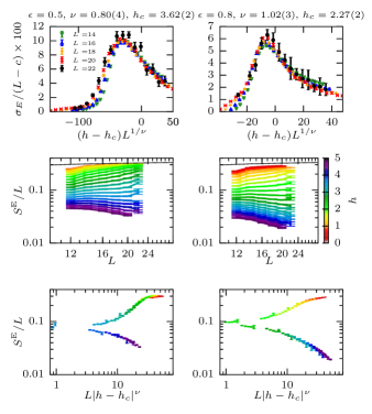
We now turn to the entanglement entropy for a real space bipartition at $L/2$ ($L$ even). Shown for two targets $\epsilon=0.5$ and $0.8$, the transition is signaled (Fig. 3) by a change in the EE scalings from volume law $S^{\rm E}/L\to{\rm constant}$ for $h<h_{c}$ to area-law with $S^{\rm E}/L\to 0$ for $h>h_{c}$. Assuming a volume law scaling at the critical point Grover , we perform a collapse of $S^{\rm E}/L$ to the form $g[L^{1/\nu}(h-h_{c})]$ (Fig. 3 bottom panel) giving estimates for the critical disorder $h_{c}$ and exponent $\nu$ consistent with other results (see Sup. Mat.). Furthermore, as recently argued Kjäll et al. (2014), the standard deviation of the entanglement entropy displays a maximum at the MBL transition. A scaling collapse of the form $\sigma_{E}=(L-c)g[L^{1/\nu}(h-h_{c})]$ (with $c$ an unknown parameter and the previous estimates of $\nu$ and $h_{c}$ from collapse of $S^{\rm E}/L$) works particularly well (top panel of Fig. 3).

Perhaps more accessible to experiments, bipartite fluctuations ${\cal F}$ of subsystem magnetization (taken here to be a half-chain $L/2$) have a similar behavior. Being simply the Curie constant of the subsystem, we also expect thermal extensivity (subextensive response) in the ergodic (localized) regime. This is clearly checked in Fig. 4 for $\epsilon=0.3$ where ${\cal F}/L$ has a crossing point at the disorder-induced MBL transition. A data collapse (inset of Fig. 4) is also possible for ${\cal F}/L=g[L^{1/\nu}(h-h_{c})])$, giving $h_{c}=3.09(7)$ and $\nu=0.77(4)$, consistent with estimates from other quantities (Fig. 1). Finally, we also performed an analysis of the dynamic fraction $f$ of an initial spin polarization Pal and Huse (2010), and obtained similar consistent scaling (see Supp. Mat. and Fig. 1).

Figure 4: Bipartite fluctuations of half-chain magnetization as a function of disorder strength at $\epsilon=0.3$. Inset: data collapse using the best estimates for the critical disorder strength $h_{c}=3.09(7)$ and $\nu=0.77(4)$.

Figure 5: Participation entropy as a function of $S_{0}^{P}=\ln(\text{dim}\mathcal{H})$ for $q=1,2$ and $\epsilon=0.4$. In the ergodic phase ($h=1.8$), $S_{q}^{P}$ grows linearly with $S_{0}^{P}$ while the linear scaling term vanishes within our error bars in the localized regime ($h=4.8$). Our fits (solid lines, see text) constrain $a_{q}\in[0,1]$ and yield a logarithmic scaling prefactor $l_{q}\approx 2(1)$ at $h=4.8$, consistent with a (slow) growth of $S_{q}^{P}$ with system size in the localized phase.

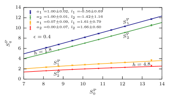
The disordered many-body system can be mapped onto a single particle problem on the complex graph spanned by the Hilbert space whose $\dim{\cal H}$ vertices are the basis states, which are connected by spin-flip terms in Eq. (1). The average coordinance of each node is $z\sim L$ and the random potential has a gaussian distribution of variance $\sigma_{h}\sim h\sqrt{L}$, meaning that the effective connectivity grows faster than the disorder strength. Using recent results on Anderson localization on Bethe lattices at large connectivity Biroli et al. (2010), we do not expect genuine Hilbert space localization at any finite disorder. This argument is corroborated by our numerical results for the PE $S_{q}^{\rm P}$ (Fig. 5) which are always found to increase with $S_{0}^{\rm P}\equiv\ln(\dim{\cal H})$, albeit much more slowly in the localized regime. Analysis of various fits of the form $S_{q}^{\rm P}=a_{q}S_{0}^{\rm P}+l_{q}\ln(S_{0}^{\rm P})+o(S_{0}^{\rm P})$ indicate that $a_{q}\simeq 1$ $\forall q$ in the ergodic regime (with possibly small negative $l_{q}$ corrections) as seen in the color scale of Fig. 1, in contrast to Anderson localization on the Bethe lattice De Luca et al. (2014). In the localized regime, we obtain essentially similar fit qualities with $a_{q}\ll 1$ (see typical numbers in Fig. 5), or $a_{q}=0$ and $l_{q}>0$ (the slow growth of $S_{q}^{\rm P}$ and our limited system sizes do not allow to separate these two possibilities).

Discussions and conclusions— Using various estimates for the MBL transition, our large-scale energy-resolved ED results indicate the existence of an extensive many-body mobility edge in the excitation spectrum (Fig. 1) of the random field Heisenberg chain. Furthermore, we show that the ergodic regime has full features of a metallic phase (with $a_{q}=1$ and GOE statistics for both energy levels and the wavefunction coefficients), and that the localized many-body states do not exhibit a true Hilbert-space localization for configuration spaces up to $\dim{\cal H}\sim 7\cdot 10^{5}$. Our detailed finite-size scaling analysis (Sup. Mat.) provides a consistent estimate of a characteristic length diverging as $|h-h_{c}|^{-\nu}$ with $\nu=0.8(3)$ through the full phase diagram. This estimate of the exponent $\nu$ appears to violate the Harris-Chayes Harris (1974); Chayes et al. (1986) criterion $\nu\geq 2/d$ (see also Ref. Kjäll et al. (2014)) within the system sizes used. This is quite intriguing given that for the same size range, the location of the critical point is consistent for all various estimates used (see Fig. 1). This opens new questions on the finite-size scaling and/or corrections to scaling at the MBL transition which may not follow Oganesyan and Huse (2007); Pal and Huse (2010) standard forms.

Besides these results for the particular model Eq. 1, we believe that the numerical techniques (massively parallel energy-resolved diagonalisation) and new indicators of the ergodic-localized transition (eigenstates correlations or bipartite fluctuations) introduced here will be useful in a large number of contexts related to MBL or ETH. In particular, the obtention of exact eigenvectors on fairly large systems will be crucial to quantify the effectiveness of encoding localized states as matrix product states, as recently advocated Friesdorf et al. ; Chandran et al. ; Pekker and Clark .

Acknowledgments — We thank G. Lemarié, F. Pollmann, B. Georgeot, O. Giraud for fruitful discussions, and CALMIP for generously providing access to the EOS supercomputer. We used the libraries PETSc, SLEPc Hernandez et al. (2005) and the MUMPS Amestoy et al. (2001, 2006) parallel solver for our calculations. This work was performed using HPC resources from GENCI (grant x2014050225) and CALMIP (grant 2014-P0677), and is supported by the French ANR program ANR-11-IS04-005-01.

Appendix A Supplementary material

A.1 Details on fitting procedures and estimates of critical exponents and fields

In order to estimate the value of the critical disorder strength $h_{c}$ and the critical exponent $\nu$, we have performed a systematic scaling analysis using the scaling ansatz $g[(h-h_{c})L^{1/\nu}]$ for the disorder averaged gap ratios ${r}$, the dynamical spin fraction ${f}$, the entanglement entropy per site $S_{\text{E}}/L$ and the bipartite fluctuations per site $\mathcal{F}/L$. We model the universal function $g$ in a window of size $2w$ centered at $h_{c}$ by a polynomial of degree three and have performed fits varying the size of the fit window and excluding system sizes smaller than $L_{\text{min}}$ for $L_{\text{min}}\in\{12,14,16\}$ in order to estimate the stability of our results. We have also tried to include drift terms in the universal function but concluded that they are not needed to obtain a very good fit quality. The results of our stability analysis is displayed in Figures 6 and 7, where we show the results of scaling fits for all quantities and fit windows. The scattering of the results can be understood as a measure of the true error bar.

Figure 6: Systematic analysis of the influence of fit windows in $h$ and $L$ on the critical disorder strength $h_{c}$. Only results for the targets $0.1$, 0.2, 0.3, 0.4, 0.5, 0.6, 0.7, 0.8 and 0.9 are shown and the symbols were slightly shifted in $\epsilon$ for better readability.

Figure 7: Systematic analysis of the influence of fit windows in $h$ and $L$ on the critical exponent $\nu$, the horizontal lines correspond to the mean value and the error bounds of our estimate for the critical exponent $\nu=0.8(3)$. Only results for the targets $0.1$, 0.2, 0.3, 0.4, 0.5, 0.6, 0.7, 0.8 and 0.9 are shown and the symbols were slightly shifted in $\epsilon$ for better readability.

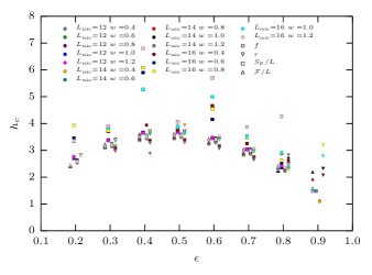
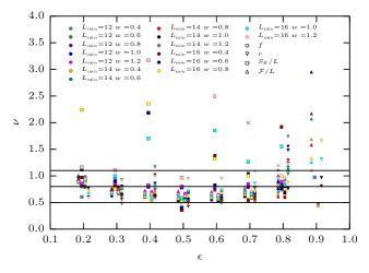
Generally, our results are all consistent and nearly all of the outliers stem from fits including only the largest system sizes $L\geq 16$, where the analysis starts to become difficult due to the reduced range in $L$. In particular, the analysis for the entanglement entropy per site is problematic in this case, as we only use even system sizes.

Additionally, at the low and high end of the spectrum, the density of states is very low, thus rendering the analysis of the gap ratios particularly problematic Oganesyan and Huse (2007).

Based on this stability analysis, we find that the fit window with $L_{\text{min}}=14$ (for the gap ratios, we use $L_{\text{min}}=15$) and $w=0.8$ seems to provide the most stable results and is therefore used for all results presented in the rest of this Letter. With the fixed fit window, we have performed a bootstrap analysis in order to estimate the statistical error of the fit parameters, in particular $h_{c}$ and $\nu$, indicated in the plots. Clearly, one has to keep in mind that on top of this error, there will be a systematic error that is of the order of the spread of the results in the stability analysis shown in this paragraph.

A.2 Dynamical spin fraction

Figure 8: ${f}$ as a function of disorder strength for different system sizes $L$ in the center of the spectrum $\epsilon=0.5$.

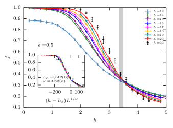
For completeness, we show here additional data for the dynamical spin fraction $f$, which has been introduced in Ref. Pal and Huse, 2010. This quantity gives a measure of how much memory of an initial spin density is lost after a long time evolution. It is $1$ (corresponding to no memory) in the ergodic phase and decays to zero in the localized phase.

It can be defined by introducing an initial spin density defined by the longest wavelength operator

$$M=\sum_{j\in[1,L]}S_{j}^{z}\exp(i2\pi j/L).$$ (2)

After evaluating the long time remainder of this spin density, one finds for the dynamic fraction for an eigenstate $|n\rangle$

$$f^{n}=1-\frac{\langle\,n\,|M^{\dagger}|n\rangle\langle\,n\,|M|n\rangle}{\langle\,n\,|M^{\dagger}M|n\rangle}.$$ (3)

Fig. 8 represents the disorder-average ${f}$ as a function of disorder strength for different system sizes $L$ in the spectrum center $\epsilon=0.5$, where a crossing point can be observed. Assuming a finite-size scaling of the form $g[(h-h_{c})L^{1/\nu}]$ allows to collapse all data (see inset), producing best-fit values of $\nu$ and $h_{c}$ (see inset) compatible with other estimates (see details of fitting procedure in first part of this Sup. Mat.).

References

- Fleishman and Anderson (1980) L. Fleishman and P. W. Anderson, Phys. Rev. B 21, 2366 (1980).
- Altshuler et al. (1997) B. L. Altshuler, Y. Gefen, A. Kamenev, and L. S. Levitov, Phys. Rev. Lett. 78, 2803 (1997).
- Jacquod and Shepelyansky (1997) P. Jacquod and D. L. Shepelyansky, Phys. Rev. Lett. 79, 1837 (1997).
- Georgeot and Shepelyansky (1998) B. Georgeot and D. L. Shepelyansky, Phys. Rev. Lett. 81, 5129 (1998).
- Gornyi et al. (2005) I. Gornyi, A. Mirlin, and D. Polyakov, Phys. Rev. Lett. 95, 206603 (2005).
- Basko et al. (2006) D. M. Basko, I. L. Aleiner, and B. L. Altshuler, Annals of Physics 321, 1126 (2006).
- Anderson (1958) P. W. Anderson, Phys. Rev. 109, 1492 (1958).
- (8) R. Nandkishore and D. A. Huse, arXiv:1404.0686 .
- (9) E. Altman and R. Vosk, arXiv:1408.2834 .
- Deutsch (1991) J. M. Deutsch, Phys. Rev. A 43, 2046 (1991).
- Srednicki (1994) M. Srednicki, Phys. Rev. E 50, 888 (1994).
- Rigol et al. (2008) M. Rigol, V. Dunjko, and M. Olshanii, Nature (London) 452, 854 (2008).
- Nandkishore et al. (2014) R. Nandkishore, S. Gopalakrishnan, and D. A. Huse, Phys. Rev. B 90, 064203 (2014).
- Serbyn et al. (2014) M. Serbyn, M. Knap, S. Gopalakrishnan, Z. Papić, N. Y. Yao, C. R. Laumann, D. A. Abanin, M. D. Lukin, and E. A. Demler, Phys. Rev. Lett. 113, 147204 (2014).
- Kwasigroch and Cooper (2014) M. P. Kwasigroch and N. R. Cooper, Phys. Rev. A 90, 021605 (2014).
- (16) N. Y. Yao, C. R. Laumann, S. Gopalakrishnan, M. Knap, M. Mueller, E. A. Demler, and M. D. Lukin, arXiv:1311.7151 .
- (17) R. Vasseur, S. A. Parameswaran, and J. E. Moore, arXiv:1407.4476 .
- Huse et al. (2013) D. A. Huse, R. Nandkishore, V. Oganesyan, A. Pal, and S. L. Sondhi, Phys. Rev. B 88, 014206 (2013).
- (19) Y. Bahri, R. Vosk, E. Altman, and A. Vishwanath, arXiv:1307.4092 .
- Chandran et al. (2014a) A. Chandran, V. Khemani, C. R. Laumann, and S. L. Sondhi, Phys. Rev. B 89, 144201 (2014a).
- Bauer and Nayak (2013) B. Bauer and C. Nayak, Journal of Statistical Mechanics: Theory and Experiment 2013, P09005 (2013).
- Vosk and Altman (2014) R. Vosk and E. Altman, Phys. Rev. Lett. 112, 217204 (2014).
- Huse et al. (2014) D. A. Huse, R. Nandkishore, and V. Oganesyan, Phys. Rev. B 90, 174202 (2014).
- Serbyn et al. (2013) M. Serbyn, Z. Papić, and D. A. Abanin, Phys. Rev. Lett. 111, 127201 (2013).
- (25) V. Ros, M. Müller, and A. Scardicchio, arXiv:1406.2175 .
- Chandran et al. (2014b) A. Chandran, I. H. Kim, G. Vidal, and D. A. Abanin, arXiv:1407.8480 (2014b).
- Oganesyan and Huse (2007) V. Oganesyan and D. A. Huse, Phys. Rev. B 75, 155111 (2007).
- Pal and Huse (2010) A. Pal and D. A. Huse, Phys. Rev. B 82, 174411 (2010).
- Žnidarič et al. (2008) M. Žnidarič, T. Prosen, and P. Prelovšek, Phys. Rev. B 77, 064426 (2008).
- Canovi et al. (2011) E. Canovi, D. Rossini, R. Fazio, G. E. Santoro, and A. Silva, Phys. Rev. B 83, 094431 (2011).
- Cuevas et al. (2012) E. Cuevas, M. Feigel’Man, L. Ioffe, and M. Mezard, Nature Communications 3, 1128 (2012).
- Kjäll et al. (2014) J. A. Kjäll, J. H. Bardarson, and F. Pollmann, Phys. Rev. Lett. 113, 107204 (2014).
- De Luca and Scardicchio (2013) A. De Luca and A. Scardicchio, EPL 101, 37003 (2013).
- Iyer et al. (2013) S. Iyer, V. Oganesyan, G. Refael, and D. A. Huse, Phys. Rev. B 87, 134202 (2013).
- Pekker et al. (2014) D. Pekker, G. Refael, E. Altman, E. Demler, and V. Oganesyan, Phys. Rev. X 4, 011052 (2014).
- (36) S. Johri, R. Nandkishore, and R. N. Bhatt, arXiv:1405.5515 .
- Bardarson et al. (2012) J. H. Bardarson, F. Pollmann, and J. E. Moore, Phys. Rev. Lett. 109, 017202 (2012).
- Andraschko et al. (2014) F. Andraschko, T. Enss, and J. Sirker, Phys. Rev. Lett. 113, 217201 (2014).
- Laumann et al. (2014) C. R. Laumann, A. Pal, and A. Scardicchio, Phys. Rev. Lett. 113, 200405 (2014).
- (40) J. M. Hickey, S. Genway, and J. P. Garrahan, arXiv:1405.5780 .
- Nanduri et al. (2014) A. Nanduri, H. Kim, and D. A. Huse, Phys. Rev. B 90, 064201 (2014).
- Bar Lev and Reichman (2014) Y. Bar Lev and D. R. Reichman, Phys. Rev. B 89, 220201 (2014).
- Note (1) We note that dynamics after a quench can be investigated on fairly large systems using methods that benefit from the low rise of entanglement in a MBL system Žnidarič et al. (2008); Bardarson et al. (2012); Andraschko et al. (2014).
- Mehta (1991) M. L. Mehta, Random matrices (Academic Press, Boston, New York, San Diego, 1991).
- Atas et al. (2013) Y. Y. Atas, E. Bogomolny, O. Giraud, and G. Roux, Phys. Rev. Lett. 110, 084101 (2013).
- Kullback and Leibler (1951) S. Kullback and R. A. Leibler, Ann. Math. Statist. 22, 79 (1951).
- Note (2) We found this numerically for eigenvectors of random matrices in the GOE ensemble, inspiring an analytical proof (O. Giraud, private communication).
- Song et al. (2012) H. F. Song, S. Rachel, C. Flindt, I. Klich, N. Laflorencie, and K. Le Hur, Phys. Rev. B 85, 035409 (2012).
- Bell (1972) R. J. Bell, Rep. Prog. Phys. 35, 1315 (1972).
- Wegner (1980) F. Wegner, Z Physik B 36, 209 (1980).
- Rodriguez et al. (2011) A. Rodriguez, L. J. Vasquez, K. Slevin, and R. A. Römer, Phys. Rev. B 84, 134209 (2011).
- Luitz et al. (2014a) D. J. Luitz, F. Alet, and N. Laflorencie, Phys. Rev. Lett. 112, 057203 (2014a).
- Luitz et al. (2014b) D. J. Luitz, N. Laflorencie, and F. Alet, Journal of Statistical Mechanics: Theory and Experiment 2014, P08007 (2014b).
- Hernandez et al. (2005) V. Hernandez, J. E. Roman, and V. Vidal, ACM Trans. Math. Software 31, 351 (2005).
- Amestoy et al. (2001) P. R. Amestoy, I. S. Duff, J. Koster, and J.-Y. L’Excellent, SIAM J. Matrix Anal. Appl. 23, 15 (2001).
- Amestoy et al. (2006) P. R. Amestoy, A. Guermouche, J.-Y. L’Excellent, and S. Pralet, Parallel Computing 32, 136 (2006).
- Page (1993) D. N. Page, Phys. Rev. Lett. 71, 1291 (1993).
- (58) T. Grover, arXiv:1405.1471 .
- Biroli et al. (2010) G. Biroli, G. Semerjian, and M. Tarzia, Progress of Theoretical Physics Supplement 184, 187 (2010).
- De Luca et al. (2014) A. De Luca, B. Altshuler, V. Kravtsov, and A. Scardicchio, Phys. Rev. Lett. 113, 046806 (2014).
- Note (3) We cannot exclude a different multifractal behavior very close to the transition.
- Harris (1974) A. B. Harris, Journal of Physics C: Solid State Physics 7, 1671 (1974).
- Chayes et al. (1986) J. T. Chayes, L. Chayes, D. S. Fisher, and T. Spencer, Phys. Rev. Lett. 57, 2999 (1986).
- (64) M. Friesdorf, A. H. Werner, W. Brown, V. B. Scholz, and J. Eisert, arXiv:1409.1252 .
- (65) A. Chandran, J. Carrasquilla, I. H. Kim, D. A. Abanin, and G. Vidal, arXiv:1410.0687 .
- (66) D. Pekker and B. K. Clark, arXiv:1410.2224 .