Ends of unimodular random manifolds

1. Introduction

A unimodular random $d$-manifold, or URM, is a random element $(M,p)$ of the space $\mathcal{M}^{d}$ of all pointed (complete, connected) Riemannian $d$-manifolds, whose law $\nu$ is a ‘unimodular’ probability measure on $\mathcal{M}^{d}$, see Definition 1. Informally, the unimodularity means that for a each fixed manifold $M$, the basepoints $p\in M$ are distributed with respect to the Riemannian volume of $M$. As explained in detail in [2], see also §1.1 below, URMs simultaneously generalize finite volume manifolds, their regular covers, randomly chosen leaves in measured foliations, and invariant random subgroups of the isometry groups of Riemannian manifolds. In this short paper, we describe the topology of the space of ends of a URM.

An end of a Riemannian manifold $M$ is called finite volume if it has a finite volume neighborhood; otherwise, it is infinite volume. The infinite volume ends of $M$ form a closed subset $\mathcal{E}_{\infty}(M)\subset\mathcal{E}(M)$ of the space of all ends. See §2.

Theorem 1.1.

If $(M,p)$ is a URM, then the following hold almost surely:

1. either $|\mathcal{E}_{\infty}(M)|=0,1,2$ or $\mathcal{E}_{\infty}(M)$ is a Cantor set,

2. if $M$ has a finite volume end, every infinite volume end of $M$ is a limit of finite volume ends,

3. setting the dimension $d=2$, if $M$ is a surface with genus $g(M)>0$, every infinite volume end of $M$ has infinite genus.

Note that the topology of a finite volume end of a Riemannian manifold can be completely arbitrary. However, if $S$ is a surface with bounded curvature, it is well-known that every finite volume end of $S$ is isolated and has a neighborhood homeomorphic to an open annulus (Lemma 2.2). Using the classification of infinite type surfaces, see §2, Theorem 1.1 implies the following:

Corollary 1.2.

Suppose $(S,p)$ is an orientable unimodular random surface with bounded curvature. Then almost surely, either

1. $S$ has finite volume and finite topological type,

2. $S$ has infinite volume and is homeomorphic to one of the following 12 surfaces: the cylinder, the plane, one of the four surfaces in Figure 1, or a surface obtained by puncturing one of these six surfaces at a locally finite set of points that intersects all end neighborhoods.

Furthermore, all these topological types can be realized by such a URS.

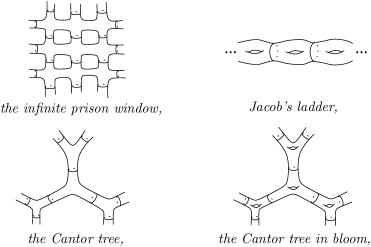
Figure 1. The Cantor tree is the boundary of a regular neighborhood of a 3-valent tree properly embedded in $\mathbb{R}^{3}$. In the spring, genus blooms near each of its vertices. The infinite prison window is also homeomorphic to the Loch Ness monster of [15] and the one-ended Jacob’s ladder.

There is a natural extension of Corollary 1.2 for non-orientable surfaces: the conclusion is that $S$ is almost surely either finite volume, one of the four surfaces of Figure 1 with sequences of non-orientable loops (and possibly punctures) exiting all its ends, or a cylinder or plane with both punctures and non-orientable loops exiting its ends. This can be proved with the same techniques as Corollary 1.2, but we will only consider orientable surfaces here for simplicity.

1.1. Motivation, definitions and applications

As mentioned above, let $\mathcal{M}^{d}$ be the space of all complete, connected, pointed Riemannian $d$-manifolds $(M,p)$, taken up to pointed isometry. We regard $\mathcal{M}^{d}$ in the smooth topology, where two pointed manifolds are close if their metrics are $C^{\infty}$-close on large diffeomorphic neighborhoods of their base points. See [2] for details. Similarly, let $\mathcal{M}^{d}_{2}$ be the space of all doubly pointed Riemannian manifolds $(M,p,q)$, taken up to doubly pointed isometry and considered in the appropriate smooth topology.

Definition 1.

A Borel probability measure $\nu$ on $\mathcal{M}^{d}$ is unimodular if and only if for every nonnegative Borel function $f:\mathcal{M}^{d}_{2}\longrightarrow\mathbb{R}$ we have

(1) $$\int_{(M,p)\in\mathcal{M}^{d}}\int_{q\in M}f(M,p,q)\,dvol\,d\nu=\int_{(M,p)\in\mathcal{M}^{d}}\int_{q\in M}f(M,q,p)\,dvol\,d\nu.$$

A unimodular random $d$-manifold (or surface, when $d=2$) is a random pointed manifold $(M,p)$ whose law is a unimodular probability measure on $\mathcal{M}^{d}$.

Equation 1 is usually called the mass transport principle, or MTP. It has its roots in foliations, but the setting in which we use it is motivated by graph theory, see Aldous-Lyons [4] and [8, 7, 17]. As an example of a unimodular measure, suppose $M$ is a finite volume Riemannian surface, and let $\mu_{M}$ be the measure on $\mathcal{M}^{d}$ obtained by pushing forward the Riemannian measure $vol$ under the map

$$M\longrightarrow\mathcal{M}^{d},\ \ \ p\longmapsto(M,p).$$

Then both sides of the MTP are equal to the integral of $f(M,p,q)$ over $(p,q)\in M\times M$, so the measure $\mu_{M}$ is unimodular, [2].

For a more general example, let $X$ be a foliated space, a separable metrizable space $X$ that is a union of ‘leaves’ that fit together locally as the horizontal factors in a product $\mathbb{R}^{d}\times Z$ for some transversal space $Z$. Suppose $X$ is Riemannian, i.e. the leaves all have Riemannian metrics, and these metrics vary smoothly in the transverse direction, see [2, §3]. There is then a leaf map

$$X\longrightarrow\mathcal{M}^{d},\ \ x\longmapsto(L_{x},x),$$

where $L_{x}$ is the leaf of $X$ through $x$. Let $\mu$ be a completely invariant probability measure on $X$: a measure obtained by integrating the Riemannian measures on the leaves of $X$ against some invariant transverse measure, see [10]. The push forward of $\mu$ under the leaf map is a unimodular measure on $\mathcal{M}^{d}$. See [2] for details.

Combining this discussion with Theorem 1.1, we get:

Theorem 1.3 (Generic leaves).

Whenever $X$ is a Riemannian foliated space with a completely invariant probability measure $\mu$, the leaf through $\mu$-almost every point $x\in X$ satisfies the conclusions (1) – (3) of Theorem 1.1.

There is a large amount of literature available concerning generic leaves of Riemannian foliated spaces, see for instance the papers by Cantwell–Conlon [11, 13, 12], Ghys [15] and Álvarez López–Candel [6], and also [5, 9, 18, 23] and [10, Chapter 3]. At least when $X$ is compact, parts (1) and (3) of Theorem 1.3 follow from Ghys’s 1995 work [15] on foliations endowed with harmonic measures, which generalize completely invariant measures. Ghys also uses classification of surfaces to prove the harmonic foliated version of Corollary 1.2.

We doubt that Theorem 1.3 is very surprising to those working in the field, but what is interesting to us is that its proof (even together with the translation from foliations to URMs in [2]) is extremely simple. In some sense, the MTP captures exactly the recurrence property necessary to prove these ‘if it happens somewhere, it happens everywhere’ statements efficiently.

Another way to construct unimodular measures on $\mathcal{M}^{d}$ is through quotients by invariant random subgroups. If $G$ is a locally compact group, let $\mathrm{Sub}_{G}$ be the space of closed subgroups of $G$ endowed with the Chabauty topology, see [1, Section 2].

Definition 2.

An invariant random subgroup (IRS) of $G$ is a random closed subgroup whose law is a conjugation invariant probability measure on $\mathrm{Sub}_{G}$.

A simple example is the IRS whose law is the unique $G$-invariant probability measure $\nu_{\Gamma}$ on the conjugacy class of a lattice $\Gamma<G$; more involved examples are given in [1, Section 12]. IRSs were first studied by Abért-Glasner-Virág [3] for discrete $G$, see also Vershik [22], and were introduced to Lie groups in [1].

In [2, §2.2], it is shown that when $X$ is a complete Riemannian manifold and $G<\mathrm{Isom}(X)$ is a subgroup such that either

1. $G$ is unimodular and act transitively on $X$, or

2. $G$ acts freely and properly discontinuously, and $G\backslash X$ has finite volume,

then any IRS $\Gamma<G$ that acts freely and properly discontinuously gives a unimodular random manifold $M=\Gamma\backslash X$, where the base point is the projection of a fixed point in $X$ in case (1), and is the projection of a randomly chosen point from a fundamental domain for the action $G\circlearrowright X$ in case (2).

All the conclusions of Theorem 1.1 then hold for these IRS quotients. So in particular, setting $G=\mathrm{PSL}_{2}\mathbb{R}$ and $X=\mathbb{H}^{2}$, we get the following, which was our initial motivation for writing this paper and was explained in the survey [20].

Corollary 1.4 (Topology of IRS quotients).

Suppose that $\Gamma$ is a discrete, torsion free IRS of $\mathrm{PSL}_{2}\mathbb{R}$. Then almost surely, the quotient $S=\Gamma\backslash\mathbb{H}^{2}$ is either finite type or is homeomorphic to one of the 12 surfaces that appear in Theorem 1.2.

Actually, only 11 surfaces appear: IRSs of $\mathrm{PSL}_{2}\mathbb{R}$ are concentrated on subgroups with full limit set, by [1, Proposition 11.3], so cannot be cyclic.

Note that any normal subgroup $H$ of a group $G$ can be considered as an IRS. So, by (2) above, any regular cover $\hat{S}$ of a (say, closed) orientable surface $S$ can be considered as a unimodular random surface, after fixing a Riemannian metric on $S$ and randomly choosing a base point for $\hat{S}$ as above. In this special case, Theorem 1.1 (1) is the classical theorem of Hopf [19] on ends of groups, and the corresponding special case of Corollary 1.2 was noticed by Grigorchuk [16].

1.2. Acknowledgements

We would like to thank Miklos Abert for helpful conversations. The first author was partially supported by NSF grant DMS 1611851.

2. Ends, bounded curvature and the proof of Corollary 1.2

Suppose that $X$ is a topological space admitting a countable cover by compact sets, e.g. any locally compact, separable space. The space of ends ${\mathcal{E}}(X)$ is then defined as the inverse limit of the system of complements of compact subsets of $X$. It is a compact, totally disconnected topological space.

More concretely, one can construct ${\mathcal{E}}(X)$ as follows. Choose a nested sequence of compact subsets $K_{1}\subset K_{2}\subset\ldots$ in $X$ such that $X=\bigcup_{i}K_{i}$. A point in ${\mathcal{E}}(X)$ is determined by a sequence $(C_{i})$, where each $C_{i}$ is a component of $X\setminus K_{i}$ and $C_{i+1}\subset C_{i}$. Moreover, for every $i$ and complementary component $C_{i}$ we get a map ${\mathcal{E}}(C_{i})\to{\mathcal{E}}(X)$, and the images of these maps are a basis for the topology.

If $X$ is an orientable surface, one can take the $K_{i}$ to be subsurfaces and define the genus of an end $(C_{i})$ as the limit of the genus of the $C_{i}$. This is either zero or infinity, and the set of ends with infinite genus is a closed set. In fact, a surface is completely determined by the genus and topology of its ends; this was originally proven by B. Kerékjártó, but a modern proof is given by I. Richards in [21]:

Theorem 2.1 (Classification of noncompact surfaces).

Suppose that $S$ and $T$ are orientable surfaces with the same genus and that there is a homeomorphism

$$\phi:{\mathcal{E}}(S)\to{\mathcal{E}}(T)$$

such that for all $\xi\in{\mathcal{E}}(S),$ the genera of $\xi$ and $\phi(\xi)$ are the same. Then $S$ and $T$ are homeomorphic.

As mentioned in the introduction, the classification of surfaces combines with Theorem 1.1 to give a classification of topological types of unimodular random surfaces of bounded curvature. The key lemma is the following:

Lemma 2.2 (Finite volume ends).

Suppose that $S$ is a complete Riemannian surface with bounded Gaussian curvatures. Then every finite volume end of $S$ has a neighborhood homeomorphic to an open annulus, and so is isolated in $\mathcal{E}(X)$.

Proof.

This is a well-known corollary of the ‘Good Choppings’ theorem of Cheeger–Gromov [14]. We may assume that $S$ itself has finite volume, by arbitrarily replacing the complement of a finite volume end neighborhood with something compact.

By [14, Theorem 0.5], $S$ is a nested union of compact subsurfaces $S_{1},S_{2},\ldots$ that are disjoint except along their boundaries, such that the boundary curves $\partial S_{i}$ have length tending to zero and uniformly bounded geodesic curvatures $\kappa$. As $S$ has finite volume, we have $\mathrm{vol}(S_{i+1}\setminus S_{i})\to 0$, and since curvature is bounded,

$$\chi(S_{i+1}\setminus S_{i})=\int_{S_{i+1}\setminus S_{i}}K\,dvol\,-\,\int_{\partial S_{i}}\kappa\,ds\to 0.$$

So for large $i$, we have that $S_{i+1}\setminus S_{i}$ is a union of annuli, and the lemma follows. ∎

To prove Corollary 1.2, then, note that if $S$ is any bounded curvature surface satisfying the conclusion of Theorem 1.1, then either $S$ has finite volume,

1. $S$ has genus zero and $\mathcal{E}(S)$ consists of either $1$ or $2$ genus zero ends,

2. $S$ has infinite genus and $\mathcal{E}(S)$ consists of either $1$ or $2$ infinite genus ends,

3. $\mathcal{E}(S)$ is a Cantor set, all of genus $0$ ends,

4. $\mathcal{E}(S)$ is a Cantor set, all of genus $\infty$ ends,

or $\mathcal{E}(S)$ is as described in one of the four cases above, except with isolated genus $0$ ends accumulating on to all the previously described ends. By classification of surfaces, this means that $S$ is as described in Theorem 1.2.

To realize all the listed topological types, we recall from [2], see also §1.1, that any regular cover of a finite volume surface can be regarded as a URS. The listed surfaces are all clearly homeomorphic to such covers.

3. The proof of Theorem 1.1

Throughout this section, let $\nu$ be a unimodular measure on $\mathcal{M}^{d}$. For clarity, we will work directly with $\nu$ here rather than referencing a $\nu$-random element of $\mathcal{M}^{d}$. We will prove the three assertions of Theorem 1.1 in turn. Each is a quick application of the mass transport principle (see Definition 1).

First, we want to show that for $\nu$-a.e. $(M,p)$, we have that $|\mathcal{E}_{\infty}(M)|=0,1,2$ or $\mathcal{E}_{\infty}(M)$ is a Cantor set. As $\mathcal{E}_{\infty}(M)$ is compact and totally disconnected, it suffices to show that it is perfect. In other words, we claim:

Lemma 3.1.

The following holds for $\nu$-a.e. $(M,p)\in\mathcal{M}^{d}$: if $M$ has an infinite volume end that is isolated in $\mathcal{E}_{\infty}(M)$, then $|\mathcal{E}_{\infty}(M)|\leq 2$.

Proof.

Throughout the proof, we can assume that $\nu$ is concentrated on infinite volume manifolds. If a pointed manifold $(M,p)$ has at least three infinite volume ends, one of which is isolated in $\mathcal{E}_{\infty}(M)$, then there are integers $r,V>0$ such that

1. $M\setminus B_{M}(p,r)$ has at least three infinite volume connected components,

2. some component of $M\setminus B_{M}(p,r)$ has a single infinite volume end,

3. the volume of $B_{M}(p,2r)$ is at most $V$.

So, it suffices to show that for each $r,V$, it is $\nu$-almost never the case that (1) – (3) hold. Define a function $f:\mathcal{M}^{d}_{2}\longrightarrow\{0,1\}$ by setting $f(M,p,q)=1$ if conditions (1) – (3) are satisfied for $(M,p)$ and if $q$ lies in one of the components from (2).

Claim 3.2.

This function $f$ is Borel.

Proof.

For each $A>0$, the condition that $M\setminus B_{M}(p,r)$ has at least three components with volume bigger than $A$, one of which contains $q$, is an open condition on $(M,p,q)\in\mathcal{M}^{d}$. So requiring (1) and (2), and also that $q$ lies in an infinite volume component of $M\setminus B_{M}(p,r)$, is an intersection of open conditions, and hence is Borel. Condition (3), that $B_{M}(p,2r)\leq V$, is closed.

Similarly, for any $R>r$, the condition that the component of $M\setminus B_{M}(p,r)$ containing $q$ contains at least two components of $M\setminus B_{M}(p,R)$ with infinite volume is Borel. Therefore, the condition $f(M,p,q)=1$ is the complement of a countable union of Borel conditions, and therefore is Borel. ∎

Claim 3.3.

If $(M,q)\in\mathcal{M}^{d}$, then $\mathrm{vol}\{p\in M\ |\ f(M,p,q)=1\}\leq V$.

Proof.

It suffices to show that $B(p_{1},r)\cap B(p_{2},r)\neq\emptyset$ whenever $f(M,p_{i},q)=1$; since then after fixing $p_{1}$, we always have $p_{2}\in B(p_{1},2r)$, so the volume estimate follows from condition (3). So, suppose the balls $B(p_{1},r)$ and $B(p_{2},r)$ are disjoint, and that $q$ is contained in components $C_{i}$ of their complements. Then either

1. $B(p_{2},r)$ separates $q$ from $p_{1}$, in which case there can only be two infinite volume components of $M\setminus B(p_{2},r)$, as in Figure 2 (a), or

2. $B(p_{2},r)$ does not separate $q$ from $p_{1}$, in which case either $C_{1}$ or $C_{2}$ has more than one infinite volume end, as in Figure 2 (b) and (c).

In both cases, though, this is a contradiction. ∎

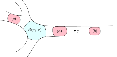
Figure 2. Here, (a), (b) and (c) indicate possible positions for $B(p_{2},r)$, relative to $B(p_{1},r)$.

The mass transport principle (MTP), see Definition 1, now states:

$$\int_{(M,q)\in\mathcal{M}^{d}}\int_{p\in M}f(M,p,q)\,dvol\,d\nu=\int_{(M,q)\in\mathcal{M}^{d}}\int_{p\in M}f(M,q,p)\,dvol\,d\nu.$$

By Claim 3.3, the inner integral on the left side of the MTP is always at most $V$, so the left side of the MTP is at most $V$. On the other hand, if $(M,q)\in\mathcal{M}^{d}$ satisfies (1) – (3), the inner integral on the right side of the MTP is clearly infinite. So, conditions (1) – (3) are $\nu$-almost never satisfied, which proves Lemma 3.1.∎

We now verify the second part of Theorem 1.1.

Lemma 3.4.

The following holds for $\nu$-a.e. $(M,p)\in\mathcal{M}^{d}$: if $M$ has a finite volume end then every infinite volume end of $M$ is a limit of finite volume ends.

Proof.

The proof is similar to that of Lemma 3.1, and we assume that the reader has understood its proof in what follows. Fixing $r,v,V>0$, the function $f:\mathcal{M}^{d}_{2}\longrightarrow\{0,1\}$ we input in the MTP is defined by setting $f(M,p,q)=1$ when

1. $q$ belongs to an infinite-volume connected component of $M\setminus B_{M}(p,r)$ that has no finite volume ends,

2. some unbounded component of $M\setminus B_{M}(p,r)$ has volume at most $v$,

3. $vol\,B_{M}(p,r)>v$, and $vol\,B_{M}(p,2r)\leq V$.

Using arguments similar to those in Claim 3.2, it is easy to show that $f$ is Borel. It suffices, then, to show that for fixed $(M,q)$, the volume of the set of all $p\in M$ for which (1) – (3) are satisfied is at most $V$, for then the lemma follows from the MTP in the same way that Lemma 3.1 did.

This also works the same way that it did in Claim 3.3. Bearing condition (3) in mind, we only have to show that if $f(M,p_{1},q)=f(M,p_{2},q)=1$ then $B_{M}(p_{1},r)\cap B_{M}(p_{2},r)\neq\emptyset$. Assume they are disjoint, and let $C_{1},C_{2}$ be the complementary components containing $q$. We now break into two cases.

1. $B_{M}(p_{2},r)\subset C_{1}$. In this case, any unbounded, finite volume component $K\subset M\setminus B_{M}(p_{2},r)$ with must contain $B_{M}(p_{1},r)$, since otherwise it is contained in $C_{2}$, which by (1) has no finite volume ends. Choosing $K$ so that $vol\,K\leq v$, this contradicts that $vol\,B_{M}(p_{1},r)>v$.

2. $B_{M}(p_{2},r)\not\subset C_{1}$. Suppose that $K\subset M\setminus B_{M}(p_{1},r)$ is an unbounded component with volume at most $v$. By volume considerations, $B_{M}(p_{2},r)$ is not contained in $K$. Hence, $K$ and $C_{1}$ are both contained in $C_{2}$, which is a contradiction since $C_{2}$ has no finite volume ends.∎

Finally, we set the dimension $d=2$, and prove the third part of Theorem 1.1.

Lemma 3.5.

The following holds for $\nu$-a.e. $(M,p)\in\mathcal{M}^{2}$: if $M$ has an infinite volume end of genus zero, then $M$ has genus zero.

Proof.

The proof is again similar to that of Lemma 3.1 and one should understand the proofs above before reading further. Fixing $r,V>0$, set $f(M,p,q)=1$ if

1. $q$ is contained in a component of $M\setminus B_{M}(p,r)$ that is infinite volume and has genus zero,

2. $B_{M}(p,r)$ contains a subsurface with positive genus

3. $vol\,B_{M}(p,2r)\leq V$.

The proof that $f$ is Borel is similar to that of Claim 3.2. It is easy to see that whenever $f(M,p_{1},q)=f(M,p_{2},q)=1$ then $B_{M}(p_{1},r)\cap B_{M}(p_{2},r)\neq\emptyset$, for if $C_{1},C_{2}$ are the complementary components containing $q$, then conditions (1) and (2) imply that neither $B_{M}(p_{1},r)\subset C_{2}$ nor $B_{M}(p_{2},r)\subset C_{1}$. As before, this implies that the set of all $p$ such that $f(M,p,q)=1$ has volume at most $V$, and the proof concludes using the MTP in the same way as it does in Lemma 3.1. ∎

References

- [1] Miklós Abért, Nicolas Bergeron, Ian Biringer, Tsachik Gelander, Nikolay Nikolov, Jean Raimbault, and Iddo Samet. On the growth of -invariants for sequences of lattices in Lie groups. arXiv:1210.2961, 2012.
- [2] Miklós Abért and Ian Biringer. Unimodular measures on the space of all Riemannian manifolds. https://arxiv.org/abs/1606.03360, 2016.
- [3] Miklós Abért, Yair Glasner, and Bálint Virág. Kesten’s theorem for invariant random subgroups. arXiv:1201.3399, 2012.
- [4] David Aldous and Russell Lyons. Processes on unimodular random networks. Electron. J. Probab., 12:no. 54, 1454–1508, 2007.
- [5] Jesús A. Álvarez López and Alberto Candel. Turbulent relations. 2012.
- [6] Jesús A. Álvarez López and Alberto Candel. Generic coarse geometry of leaves. 2014.
- [7] I. Benjamini, R. Lyons, Y. Peres, and O. Schramm. Group-invariant percolation on graphs. Geom. Funct. Anal., 9(1):29–66, 1999.
- [8] Itai Benjamini and Oded Schramm. Recurrence of distributional limits of finite planar graphs. Electron. J. Probab., 6:no. 23, 13 pp. (electronic), 2001.
- [9] Miguel Bermúdez and Gilbert Hector. Laminations hyperfinies et revêtements. Ergodic Theory Dynam. Systems, 26(2):305–339, 2006.
- [10] Alberto Candel and Lawrence Conlon. Foliations. II, volume 60 of Graduate Studies in Mathematics. American Mathematical Society, Providence, RI, 2003.
- [11] John Cantwell and Lawrence Conlon. Endsets of leaves. Topology, 21(4):333–352, 1982.
- [12] John Cantwell and Lawrence Conlon. Generic leaves. Comment. Math. Helv., 73(2):306–336, 1998.
- [13] John Cantwell and Lawrence Conlon. Endsets of exceptional leaves; a theorem of G. Duminy. In Foliations: geometry and dynamics (Warsaw, 2000), pages 225–261. World Sci. Publ., River Edge, NJ, 2002.
- [14] Jeff Cheeger and Mikhael Gromov. Chopping Riemannian manifolds. In Differential geometry, volume 52 of Pitman Monogr. Surveys Pure Appl. Math., pages 85–94. Longman Sci. Tech., Harlow, 1991.
- [15] Étienne Ghys. Topologie des feuilles génériques. Ann. of Math. (2), 141(2):387–422, 1995.
- [16] R. I. Grigorchuk. Topological and metric types of surfaces that regularly cover a closed surface. Izv. Akad. Nauk SSSR Ser. Mat., 53(3):498–536, 671, 1989.
- [17] Olle Häggström. Infinite clusters in dependent automorphism invariant percolation on trees. Ann. Probab., 25(3):1423–1436, 1997.
- [18] Gilbert Hector, Shigenori Matsumoto, and Gaël Meigniez. Ends of leaves of Lie foliations. J. Math. Soc. Japan, 57(3):753–779, 2005.
- [19] Heinz Hopf. Enden offener Räume und unendliche diskontinuierliche Gruppen. Comment. Math. Helv., 16:81–100, 1944.
- [20] Jean Raimbault. Géométrie et topologie des variétés hyperboliques de grand volume. Séminaire de Théorie spectrale et géométrie (Grenoble), 31, 2012-2014.
- [21] Ian Richards. On the classification of noncompact surfaces. Trans. Amer. Math. Soc., 106:259–269, 1963.
- [22] Anatolii Moiseevich Vershik. Totally nonfree actions and the infinite symmetric group. Moscow Mathematical Journal, 12(1):193–212, 2012.
- [23] Paweł Walczak. Dynamics of foliations, groups and pseudogroups, volume 64 of Instytut Matematyczny Polskiej Akademii Nauk. Monografie Matematyczne (New Series) [Mathematics Institute of the Polish Academy of Sciences. Mathematical Monographs (New Series)]. Birkhäuser Verlag, Basel, 2004.