Multivariate Response and Parsimony for Gaussian Cluster-Weighted Models

Abstract

A family of parsimonious Gaussian cluster-weighted models is presented. This family concerns a multivariate extension to cluster-weighted modelling that can account for correlations between multivariate responses. Parsimony is attained by constraining parts of an eigen-decomposition imposed on the component covariance matrices. A sufficient condition for identifiability is provided and an expectation-maximization algorithm is presented for parameter estimation. Model performance is investigated on both synthetic and classical real data sets and compared with some popular approaches. Finally, accounting for linear dependencies in the presence of a linear regression structure is shown to offer better performance, vis-à-vis clustering, over existing methodologies.

1 Introduction

Mixture models have seen increasing use over the decade or two, with many important applications in clustering and classification (examples include: Hennig and Liao, 2013, Lee and McLachlan, 2013, Andrews and McNicholas, 2014, Biernacki and Lourme, 2014, Browne and McNicholas, 2014b, Bouveyron and Brunet-Saumard, 2014, Lin et al., 2014, Franczak et al., 2015, Wei and McNicholas, 2015, Anderlucci and Viroli, 2015, O’Hagan et al., 2016, and McNicholas, 2016). Arguably, the most famous model-based clustering methodology is the Gaussian parsimonious clustering models (GPCM) family (Celeux and Govaert, 1995), which is supported by the mclust (Fraley and Raftery, 2002; Fraley et al., 2012), mixture (Browne and McNicholas, 2015), and Rmixmod (Lebret et al., 2015) packages for R (R Core Team, 2015). However, such models do not typically account for dependencies via covariates. When there is a clear regression relationship between some variables, important insight can be gained by accounting for functional dependencies between those variables. For such data, traditional model-based clustering methods that fail to incorporate such a relationship may not perform as well.

Some popular mixture-based methodologies that deal with regression data are finite mixtures of regression (FMR; DeSarbo and Cron, 1988) and finite mixtures of regression with concomitant variables (FMRC; Wedel, 2002), supported by the flexmix (Leisch, 2004; Grün and Leisch, 2008) package for R. FMR only model the distribution of the response given the covariates, whereas FMRC also model the mixing weights of the components as a multinomial logistic model of some concomitant variables (which are often the covariate variables). However, these methodologies do not explicitly use the distribution of the covariates for clustering, i.e., the assignment of data points to clusters does not directly utilize any information from the distribution of the covariates. Recently, finite mixtures of seemingly unrelated linear regressions have also been proposed (Galimberti et al., 2015).

A flexible framework for density estimation and clustering of data with local functional dependencies is represented by the cluster-weighted model (CWM; Gershenfeld, 1997), also called the saturated mixture regression model by Wedel (2002). CWMs were first investigated in a general statistical mixture framework by Ingrassia et al. (2012). The same paper presented theoretical and numerical properties, and discussed the performance of the model under both Gaussian and $t$-distributional assumptions (see also Ingrassia et al., 2014). As opposed to FMR and FMRC, CWMs allow for assignment dependence (cf. Hennig, 2000), i.e., the assignment of an observation to a cluster is also dependent on the distribution of the covariates. In such models, the component covariate distributions can be distinct; for a discussion about the difference between FMR, FMRC, and CWMs from a geometrical point of view, see Ingrassia and Punzo (2016). Some extensions of this methodology have dealt with non-linear local relationships (Punzo, 2014), high dimensional covariates (Subedi et al., 2013, 2015), and various response types (Ingrassia et al., 2015; Punzo and Ingrassia, 2013, 2015).

In this paper, a family of parsimonious Gaussian CWMs is presented. It concerns multivariate response, while CWMs have so far only dealt with univariate response. Note that parsimony is vital in real data applications and this is the first time that CWMs are being used with eigen-decomposed covariance structures. Regarding multivariate response in the FMR and FMRC framework, using multivariate response is possible in flexmix but the package currently does not account for correlated response variables, i.e., these models assume independence between the response variables. FMR models that deal with correlated response variables have been recently proposed (Soffritti and Galimberti, 2011; Galimberti and Soffritti, 2013), but these models do not decompose the covariance structure nor do they use information from the distribution of the covariates. Furthermore, these papers do not investigate FMRC models that deal with correlated responses. Families of eigen-decomposed parsimonious FMR and FMRC models that can account for correlated response variables have been recently proposed (eFMR and eFMRC; Dang and McNicholas, 2015); however, these models do not take into account the distribution of the covariates.

For the proposed multivariate response CWM, parsimonious models are developed by constraining parts of an eigen-decomposition imposed on the component covariance matrices of both the responses and the covariates. This family of parsimonious models is referred to as the eigen-decomposed multivariate response CWM (eMCWM). The Bayesian information criterion (BIC; Schwarz, 1978) and the integrated completed likelihood (ICL; Biernacki et al., 2000) are considered for model selection on this family. Comparisons to FMR, FMRC, eFMR, eFMRC, and GPCMs are made. Note that, hereafter, FMR and FMRC models as implemented in flexmix will simply be referred to as the FMR and FMRC models, respectively.

The remainder of the paper is organized as follows. In Section 2, basic ideas on CWMs are summarized. In Section 3, we recall an eigen-decomposition of a covariance matrix. Identifiability is treated in Section 4. An expectation-maximization (EM) algorithm for maximum likelihood parameter estimation is presented in Section 5. Moreover, issues of model selection, algorithm initialization, convergence criterion, and performance assessment are also discussed. In Section 6, results of numerical studies based on both real and simulated data are presented. Finally, in Section 7, some conclusions and ideas for future research are discussed.

2 Cluster-weighted models

Multivariate correlated responses can be conveniently accounted for in a CWM framework. Let $\boldsymbol{X}$ and $\boldsymbol{Y}$ be random vectors defined on $\Omega$ with joint probability distribution $p(\boldsymbol{x},\boldsymbol{y})$. Here, the response vector $\boldsymbol{Y}$ has values in $\mathbb{R}^{d}$ and the vector of covariates $\boldsymbol{X}$ has values in $\mathbb{R}^{p}$. Let $\Omega$ be partitioned into $G$ disjoint groups, such that $\Omega=\Omega_{1}\cup\cdots\cup\Omega_{G}$. Then, in a CWM framework, the joint probability $p(\boldsymbol{x},\boldsymbol{y})$ can be decomposed as

$$p(\boldsymbol{x},\boldsymbol{y})=\sum^{G}_{g=1}p(\boldsymbol{y}|\boldsymbol{x},\Omega_{g})p(\boldsymbol{x}|\Omega_{g})\pi_{g},$$ (1)

where $p(\boldsymbol{y}|\boldsymbol{x},\Omega_{g})$ is the conditional density of the multivariate response $\boldsymbol{Y}$ given the covariates $\boldsymbol{X}$ and $\Omega_{g}$, $p(\boldsymbol{X}|\Omega_{g})$ is the probability density of $\boldsymbol{X}$ given $\Omega_{g}$, and $\pi_{g}=p(\Omega_{g})$ are the mixing weights, where $\pi_{g}>0$ and $\sum^{G}_{g=1}\pi_{g}=1$, $g=1,\ldots,G$. Here, $\boldsymbol{X}|\Omega_{g}$ is assumed to be normally distributed with mean $\boldsymbol{\mu}_{\boldsymbol{X}g}$ and covariance matrix $\boldsymbol{\Sigma}_{\boldsymbol{X}g}$, and $\boldsymbol{Y}|(\boldsymbol{X}=\boldsymbol{x},\Omega_{g})$ is assumed to be normally distributed with conditional mean $\boldsymbol{\mu}_{\boldsymbol{Y}}\left(\boldsymbol{x}|\boldsymbol{B}_{g}\right)$, given by some linear transformation of $\boldsymbol{X}$, and covariance matrix $\boldsymbol{\Sigma}_{\boldsymbol{Y}g}$, $g=1,\ldots,G$. Here, $\boldsymbol{\mu}_{\boldsymbol{Y}}\left(\boldsymbol{x}|\boldsymbol{B}_{g}\right)=\boldsymbol{B}^{\prime}_{g}\boldsymbol{x}^{*}$ is used where $\boldsymbol{B}_{g}\in\mathbb{R}^{(1+p)\times d}$ and $\boldsymbol{x}^{*}=\left(1,\boldsymbol{x}^{\prime}\right)^{\prime}$. Hence, $\boldsymbol{Y}$ ($\boldsymbol{X}$) is a matrix of $N$ observations on $d$ ($p+1$) response variables while $\boldsymbol{B}$ for a specific component $g$ is a $p+1$ by $d$ matrix of regression coefficients with one column for each response variable. Then, model (1) can be rewritten as

$$p\left(\boldsymbol{x},\boldsymbol{y}|\boldsymbol{\vartheta}\right)=\sum^{G}_{g=1}\phi_{d}\left(\boldsymbol{y}|\boldsymbol{x},\boldsymbol{\mu}_{\boldsymbol{Y}}(\boldsymbol{x}|\boldsymbol{B}_{g}),\boldsymbol{\Sigma}_{\boldsymbol{Y}g}\right)\phi_{p}\left(\boldsymbol{x}|\boldsymbol{\mu}_{\boldsymbol{X}g},\boldsymbol{\Sigma}_{\boldsymbol{X}g}\right)\pi_{g},$$ (2)

where $\phi_{d}$ ($\phi_{p}$) represents the density of a $d$-variate ($p$-variate) Gaussian random vector and $\boldsymbol{\vartheta}$ denotes the set of all parameters.

3 Parsimonious Models

For a single $q\times q$ covariance matrix, the number of free parameters increases quadratically with the dimensionality $q$. In model-based clustering, parsimony is usually necessary for real applications. Parsimony can be introduced by constraining parts of a particular decomposition of a covariance matrix (Celeux and Govaert, 1995; McNicholas et al., 2010; Punzo et al., 2016). An eigen-decomposition of such a matrix (cf. Celeux and Govaert, 1995) yields

$$\boldsymbol{\Sigma}_{g}=\lambda_{g}\boldsymbol{\Gamma}_{g}\boldsymbol{\Delta}_{g}\boldsymbol{\Gamma}_{g}^{\prime},$$

for $g=1,\ldots,G$, where $\lambda_{g}=\left|\boldsymbol{\Sigma}_{g}\right|^{1/q}$ is a constant, $\boldsymbol{\Delta}_{g}$ is a diagonal matrix with entries (sorted in decreasing order) proportional to the eigenvalues of $\boldsymbol{\Sigma}_{g}$ with the constraint $|\boldsymbol{\Delta}_{g}|=1$, and $\boldsymbol{\Gamma}_{g}$ is a $q\times q$ orthogonal matrix of the eigenvectors (ordered according to the eigenvalues) of $\boldsymbol{\Sigma}_{g}$. Geometrically, $\lambda_{g}$ determines the volume, $\boldsymbol{\Delta}_{g}$ the shape, and $\boldsymbol{\Gamma}_{g}$ the orientation of the $g$th component. By constraining $\lambda_{g}$, $\boldsymbol{\Gamma}_{g}$, and $\boldsymbol{\Delta}_{g}$ to be equal or variable across groups, a family of fourteen models (Table 1) is obtained. This family can be further split into three subfamilies. Here, the EII and VII models belong to the spherical family, the models with an axis-aligned orientation belong to the diagonal family, while the rest of the models belong to the general family.

Table 1: Geometric interpretation and the number of free parameters in the eigen-decomposed covariance structures.

Model	Volume	Shape	Orientation	$\boldsymbol{\Sigma}_{g}$	Free Cov. Parameters
EII	Equal	Spherical	-	$\lambda\boldsymbol{I}$	1
VII	Variable	Spherical	-	$\lambda_{g}\boldsymbol{I}$	$G$
EEI	Equal	Equal	Axis-Aligned	$\lambda\boldsymbol{\Delta}$	$q$
VEI	Variable	Equal	Axis-Aligned	$\lambda_{g}\boldsymbol{\Delta}$	$G+q-1$
EVI	Equal	Variable	Axis-Aligned	$\lambda\boldsymbol{\Delta}_{g}$	$Gq-(G-1)$
VVI	Variable	Variable	Axis-Aligned	$\lambda_{g}\boldsymbol{\Delta}_{g}$	$Gq$
EEE	Equal	Equal	Equal	$\lambda\boldsymbol{\Gamma}\boldsymbol{\Delta}\boldsymbol{\Gamma}^{\prime}$	$q\left(q+1\right)/2$
VEE	Variable	Equal	Equal	$\lambda_{g}\boldsymbol{\Gamma}\boldsymbol{\Delta}\boldsymbol{\Gamma}^{\prime}$	$q(q+1)/2+(G-1)$
EVE	Equal	Variable	Equal	$\lambda\boldsymbol{\Gamma}\boldsymbol{\Delta}_{g}\boldsymbol{\Gamma}^{\prime}$	$q(q+1)/2+(G-1)(q-1)$
EEV	Equal	Equal	Variable	$\lambda\boldsymbol{\Gamma}_{g}\boldsymbol{\Delta}\boldsymbol{\Gamma}_{g}^{\prime}$	$Gq(q+1)/2-(G-1)q$
VVE	Variable	Variable	Equal	$\lambda_{g}\boldsymbol{\Gamma}\boldsymbol{\Delta}_{g}\boldsymbol{\Gamma}^{\prime}$	$q(q+1)/2+(G-1)q$
VEV	Variable	Equal	Variable	$\lambda_{g}\boldsymbol{\Gamma}_{g}\boldsymbol{\Delta}\boldsymbol{\Gamma}_{g}^{\prime}$	$Gq(q+1)/2-(G-1)(q-1)$
EVV	Equal	Variable	Variable	$\lambda\boldsymbol{\Gamma}_{g}\boldsymbol{\Delta}_{g}\boldsymbol{\Gamma}_{g}^{\prime}$	$Gq(q+1)/2-(G-1)$
VVV	Variable	Variable	Variable	$\lambda_{g}\boldsymbol{\Gamma}_{g}\boldsymbol{\Delta}_{g}\boldsymbol{\Gamma}_{g}^{\prime}$	$Gq\left(q+1\right)/2$

Here, the covariance matrices $\boldsymbol{\Sigma}_{\boldsymbol{X}g}$ and $\boldsymbol{\Sigma}_{\boldsymbol{Y}g}$ in (2) are decomposed. Constraining $\lambda_{g}$, $\boldsymbol{\Gamma}_{g}$, and $\boldsymbol{\Delta}_{g}$ on these decompositions in Equation (2) leads to 14 different covariance structures for both $\boldsymbol{X}$ and $\boldsymbol{Y}$, resulting in a total of $14\times 14=196$ models. This is the eMCWM family. Note that for the purposes of notation, an eMCWM with a VEV covariance structure for $\boldsymbol{Y}|\boldsymbol{X}=\boldsymbol{x}$ and an EII covariance structure for $\boldsymbol{X}$ will be denoted as a VEV-EII model.

4 Identifiability

Identifiability is important for parameter inference and for the usual asymptotic theory to hold for maximum likelihood estimation of the model parameters (cf. Section 5). Proof of the identifiability of univariate and multivariate finite Gaussian mixture distributions is provided by Teicher (1963) and Yakowitz and Spragins (1968), respectively, while general conditions for identifiability of mixtures of linear models can be found in Hennig (2000). Proof of the identifiability of the generalized linear Gaussian CWM has recently been provided by Ingrassia et al. (2015). Here, identification conditions are provided for the multivariate response (Gaussian) CWM defined in (2).

Generally speaking, identifiability for mixture models can be defined as follows. Consider a parametric class of density (probability) functions $\mathcal{F}=\left\{f(\boldsymbol{z}|\boldsymbol{\psi})\,:\,\boldsymbol{z}\in\mathcal{Z}\,,\,\boldsymbol{\psi}\in\boldsymbol{\Psi}\right\}$. Then, the class of finite mixtures of functions in $\mathcal{F}$ is

$$\mathcal{H} =\biggl{\{}h(\boldsymbol{z}|\boldsymbol{\vartheta})\,:\,h(\boldsymbol{z}|\boldsymbol{\vartheta})=\sum_{g=1}^{G}f(\boldsymbol{z}|\boldsymbol{\psi}_{g})\pi_{g},\,\mbox{ with }\,\pi_{g}>0\,\mbox{ and }\,\sum_{g=1}^{G}\pi_{g}=1,$$

$$\qquad f(\cdot|\boldsymbol{\psi}_{g})\in\mathcal{F},g=1,\ldots,G,\boldsymbol{\psi}_{g}\neq\boldsymbol{\psi}_{j}\mbox{ for }g\neq j,\,G\in\mathbb{N},\,\boldsymbol{z}\in\mathcal{Z}\,,\,\boldsymbol{\vartheta}\in\boldsymbol{\varTheta}\biggr{\}}.$$

This class is identifiable if for any two members

$$h(\boldsymbol{z}|\boldsymbol{\vartheta})=\sum_{g=1}^{G}f(\boldsymbol{z}|\boldsymbol{\psi}_{g})\pi_{g}\quad\mbox{and}\quad h(\boldsymbol{z}|\widetilde{\boldsymbol{\vartheta}})=\sum_{s=1}^{\widetilde{G}}f(\boldsymbol{z}|\widetilde{\boldsymbol{\psi}}_{s})\widetilde{\pi}_{s}$$

of $\mathcal{H}$, $h(\boldsymbol{z}|\boldsymbol{\vartheta})=h(\boldsymbol{z}|\widetilde{\boldsymbol{\vartheta}})$ implies that $G=\widetilde{G}$, and for each $g\in\{1,\ldots,G\}$ there exists $s\in\{1,\ldots,G\}$ such that $\pi_{g}=\widetilde{\pi}_{s}$ and $\boldsymbol{\psi}_{g}=\widetilde{\boldsymbol{\psi}}_{s}$.

In Theorem 1, a sufficient identification condition is provided for the most general eMCWM (i.e., the VVV-VVV model). In particular, a sufficient condition for the identifiability of the class $\mathcal{C}$ is established where

$$\mathcal{C} =\biggl{\{}p(\boldsymbol{x},\boldsymbol{y}|\boldsymbol{\vartheta})\,:\,p(\boldsymbol{x},\boldsymbol{y}|\boldsymbol{\vartheta})=\sum^{G}_{g=1}\phi_{d}\left(\boldsymbol{y}|\boldsymbol{x},\boldsymbol{\mu}_{\boldsymbol{Y}}\left(\boldsymbol{x}|\boldsymbol{B}_{g}\right),\boldsymbol{\Sigma}_{\boldsymbol{Y}g}\right)\phi_{p}(\boldsymbol{x}|\boldsymbol{\mu}_{\boldsymbol{X}g},\boldsymbol{\Sigma}_{\boldsymbol{X}g})\pi_{g},\biggr{.}$$

$$\qquad\biggl{.}\text{ with }\pi_{g}>0,\sum_{g=1}^{G}\pi_{g}=1,\,(\boldsymbol{B}_{g},\boldsymbol{\Sigma}_{\boldsymbol{Y}g})\neq(\boldsymbol{B}_{j},\boldsymbol{\Sigma}_{\boldsymbol{Y}j})\mbox{ for }g\neq j,\,\left(\boldsymbol{x},\boldsymbol{y}\right)\in\mathbb{R}^{p+d}\,,\,\biggr{.}$$

$$\qquad\biggl{.}\boldsymbol{\vartheta}=\{\boldsymbol{B}_{g},\boldsymbol{\Sigma}_{\boldsymbol{Y}g},\boldsymbol{\mu}_{\boldsymbol{X}g},\boldsymbol{\Sigma}_{\boldsymbol{X}g},\pi_{g};g=1,\ldots,G\}\in\boldsymbol{\varTheta},G\in\mathbb{N}\,\biggr{\}}.$$ (3)

In the following theorem, a sufficient condition for $\mathcal{C}$ to be identifiable in $\mathcal{X}\times\mathbb{R}^{d}$ is provided, where $\mathcal{X}\subseteq\mathbb{R}^{p}$ is a set having probability one according to the multivariate Gaussian density $\phi_{p}$.

In other words, this proves that the class $\mathcal{C}$ is identifiable for almost all $\boldsymbol{x}\in\mathbb{R}^{p}$ and for all $\boldsymbol{y}\in\mathbb{R}^{d}$.

Theorem 1.

Let $\mathcal{C}$ be the class defined in (3) and assume that there exists a set $\mathcal{X}\subseteq\mathbb{R}^{p}$ having probability equal to one according to the $p$-variate Gaussian distribution such that the mixture of regression models

$$\sum_{g=1}^{G}\phi_{d}\left(\boldsymbol{y}|\boldsymbol{x},\boldsymbol{\mu}_{\boldsymbol{Y}}\left(\boldsymbol{x}|\boldsymbol{B}_{g}\right),\boldsymbol{\Sigma}_{\boldsymbol{Y}g}\right)\alpha_{g}\left(\boldsymbol{x}\right),\quad\boldsymbol{y}\in\mathbb{R}^{d},$$ (4)

is identifiable for each fixed $\boldsymbol{x}\in\mathcal{X}$, where $\alpha_{1}(\boldsymbol{x}),\ldots,\alpha_{G}(\boldsymbol{x})$ are positive weights summing to one for each $\boldsymbol{x}\in\mathcal{X}$. Then, the class $\mathcal{C}$ is identifiable in $\mathcal{X}\times\mathbb{R}^{d}$.

Proof.

The proof is given in Appendix A. ∎

5 Inference

5.1 Parameter Estimation for eMCWM

Parameter estimation, via the EM algorithm of Dempster et al. (1977), is described here for the unconstrained VVV-VVV model from the eMCWM family. Details on alternative algorithms to find maximum likelihood estimates of a mixture distribution can be found in Böhning (1995, 2003). Let $\mathcal{S}=\left\{(\boldsymbol{x}_{1},\boldsymbol{y}_{1}),\ldots,(\boldsymbol{x}_{N},\boldsymbol{y}_{N})\right\}$ be a sample of $N$ independent observations from model (2). Then, the incomplete-data likelihood function is

$$L\left(\boldsymbol{\vartheta}|\mathcal{S}\right)=\prod_{i=1}^{N}p(\boldsymbol{x}_{i},\boldsymbol{y}_{i}|\boldsymbol{\vartheta})=\prod_{i=1}^{N}\left[\sum_{g=1}^{G}\phi_{d}(\boldsymbol{y}_{i}|\boldsymbol{\mu}_{\boldsymbol{Y}}(\boldsymbol{x}_{i}|\boldsymbol{B}_{g}),\boldsymbol{\Sigma}_{\boldsymbol{Y}g})\phi_{p}(\boldsymbol{x}_{i}|\boldsymbol{\mu}_{\boldsymbol{X}g},\boldsymbol{\Sigma}_{\boldsymbol{X}g})\pi_{g}\right].$$

Note that $\mathcal{S}$ is considered incomplete in the context of the EM algorithm. The complete-data are $\mathcal{S}_{\text{c}}=\left\{(\boldsymbol{x}_{1},\boldsymbol{y}_{1},\boldsymbol{z}_{1}),\ldots,(\boldsymbol{x}_{N},\boldsymbol{y}_{N},\boldsymbol{z}_{N})\right\}$, where the missing variable $\boldsymbol{z}_{i}$ is the component label vector such that $z_{ig}$ = 1 if $(\boldsymbol{x}_{i},\boldsymbol{y}_{i})$ belongs to the $g$th component and $z_{ig}=0$ otherwise. Now, the corresponding complete-data likelihood is

$$L_{c}\left(\boldsymbol{\vartheta}|\mathcal{S}_{\text{c}}\right)=\prod_{i=1}^{N}\prod_{g=1}^{G}[\phi_{d}(\boldsymbol{y}_{i}|\boldsymbol{\mu}_{\boldsymbol{Y}}(\boldsymbol{x}_{i}|\boldsymbol{B}_{g}),\boldsymbol{\Sigma}_{\boldsymbol{Y}g})\phi_{p}(\boldsymbol{x}_{i}|\boldsymbol{\mu}_{\boldsymbol{X}g},\boldsymbol{\Sigma}_{\boldsymbol{X}g})\pi_{g}]^{z_{ig}}.$$

The complete-data log-likelihood function can be decomposed as

$$l_{c}\left(\boldsymbol{\vartheta}|\mathcal{S}_{\text{c}}\right)=\sum_{i=1}^{N}\sum_{g=1}^{G}z_{ig}\left[\log\phi_{d}(\boldsymbol{y}_{i}|\boldsymbol{\mu}_{\boldsymbol{Y}}(\boldsymbol{x}_{i}|\boldsymbol{B}_{g}),\boldsymbol{\Sigma}_{\boldsymbol{Y}g})+\log\phi_{p}(\boldsymbol{x}_{i}|\boldsymbol{\mu}_{\boldsymbol{X}g},\boldsymbol{\Sigma}_{\boldsymbol{X}g})+\log\pi_{g}\right].$$

The E-step involves calculating the expected complete-data log-likelihood

$$Q\left(\boldsymbol{\vartheta}|\boldsymbol{\vartheta}^{(k)}\right) =\mathbb{E}_{\boldsymbol{\vartheta}^{(k)}}\left\{l_{c}\left(\boldsymbol{\vartheta}|\mathcal{S_{\text{c}}}\right)\right\}$$

$$=\sum_{i=1}^{N}\sum_{g=1}^{G}\hat{z}_{ig}^{(k)}\left[Q_{1}\left(\boldsymbol{B}_{g},\boldsymbol{\Sigma}_{\boldsymbol{Y}g}|\boldsymbol{\vartheta}^{(k)}\right)+Q_{2}\left(\boldsymbol{\mu}_{\boldsymbol{X}g},\boldsymbol{\Sigma}_{\boldsymbol{X}g}|\boldsymbol{\vartheta}^{(k)}\right)+\log\pi_{g}^{(k)}\right],$$

where

$$\hat{z}_{ig}^{(k)}=\mathbb{E}_{\boldsymbol{\vartheta}^{(k)}}\{Z_{ig}|\boldsymbol{x}_{i},\boldsymbol{y}_{i}\}=\frac{\phi_{d}(\boldsymbol{y}_{i}|\boldsymbol{\mu}_{\boldsymbol{Y}}(\boldsymbol{x}_{i}|\boldsymbol{B}_{g}^{(k)}),\boldsymbol{\Sigma}_{\boldsymbol{Y}g}^{(k)})\phi_{p}(\boldsymbol{x}_{i}|\boldsymbol{\mu}_{\boldsymbol{X}g}^{(k)},\boldsymbol{\Sigma}_{\boldsymbol{X}g}^{(k)})\pi_{g}^{(k)}}{\displaystyle\sum_{j=1}^{G}\phi_{d}(\boldsymbol{y}_{i}|\boldsymbol{\mu}_{\boldsymbol{Y}}(\boldsymbol{x}_{i}|\boldsymbol{B}_{j}^{(k)}),\boldsymbol{\Sigma}_{\boldsymbol{Y}j}^{(k)})\phi_{p}(\boldsymbol{x}_{i}|\boldsymbol{\mu}_{\boldsymbol{X}j}^{(k)},\boldsymbol{\Sigma}_{\boldsymbol{X}j}^{(k)})\pi_{j}^{(k)}}$$

provides the current value of $z_{ig}$ on the $k^{\text{th}}$-iteration and

$$Q_{1}\left(\boldsymbol{B}_{g},\boldsymbol{\Sigma}_{\boldsymbol{Y}g}|\boldsymbol{\vartheta}^{(k)}\right) =\frac{1}{2}\left[-d\log\left(2\pi\right)-\log|\boldsymbol{\Sigma}_{\boldsymbol{Y}g}^{(k)}|-\left(\boldsymbol{y}_{i}-\boldsymbol{B}^{{}^{\prime}(k)}_{g}\boldsymbol{x}_{i}^{*}\right)^{\prime}\boldsymbol{\Sigma}_{\boldsymbol{Y}g}^{(k)(-1)}(\boldsymbol{y}_{i}-\boldsymbol{B}^{{}^{\prime}(k)}_{g}\boldsymbol{x}_{i}^{*})\right],$$

$$Q_{2}\left(\boldsymbol{\mu}_{\boldsymbol{X}g},\boldsymbol{\Sigma}_{\boldsymbol{X}g}|\boldsymbol{\vartheta}^{(k)}\right) =\frac{1}{2}\left[-p\log\left(2\pi\right)-\log|\boldsymbol{\Sigma}_{\boldsymbol{X}g}^{(k)}|-\left(\boldsymbol{x}_{i}-\boldsymbol{\mu}_{\boldsymbol{X}g}^{(k)}\right)^{\prime}\boldsymbol{\Sigma}_{\boldsymbol{X}g}^{(k)(-1)}\left(\boldsymbol{x}_{i}-\boldsymbol{\mu}_{\boldsymbol{X}g}^{(k)}\right)\right].$$

The M-step on the $(k+1)^{\text{th}}$ iteration of the EM algorithm involves the maximization of the conditional expectation of the complete-data log-likelihood with respect to $\boldsymbol{\vartheta}$. The update for $\pi_{g}^{(k+1)}$ is

$$\hat{\pi}_{g}^{(k+1)}=\frac{1}{N}\sum_{i=1}^{N}\hat{z}_{ig}^{(k)}.$$ (5)

The updates for $\boldsymbol{\mu}_{\boldsymbol{X}g}^{(k+1)}$ and $\boldsymbol{\Sigma}_{\boldsymbol{X}g}^{(k+1)}$, $g=1,\ldots,G$, are

$$\hat{\boldsymbol{\mu}}_{\boldsymbol{X}g}^{(k+1)} =\frac{\sum_{i=1}^{N}\hat{z}_{ig}^{(k)}\boldsymbol{x}_{i}}{\sum_{i=1}^{N}\hat{z}_{ig}^{(k)}},$$ (6)

$$\hat{\boldsymbol{\Sigma}}_{\boldsymbol{X}g}^{(k+1)} =\frac{\sum_{i=1}^{N}\hat{z}_{ig}^{(k)}\left(\boldsymbol{x}_{i}-\hat{\boldsymbol{\mu}}_{\boldsymbol{X}g}^{(k+1)}\right)\left(\boldsymbol{x}_{i}-\hat{\boldsymbol{\mu}}_{\boldsymbol{X}g}^{(k+1)}\right)^{\prime}}{\sum_{i=1}^{N}\hat{z}_{ig}^{(k)}}.$$ (7)

These closed form updates can also be found in McLachlan and Peel (2000). The updates for $\boldsymbol{B}_{g}^{(k+1)}$ and $\boldsymbol{\Sigma}_{\boldsymbol{Y}g}^{(k+1)}$ (see Appendix B for details), $g=1,\ldots,G$, are

$$\hat{\boldsymbol{B}}_{g}^{(k+1)^{\prime}}=\left(\sum_{i=1}^{N}\hat{z}_{ig}^{(k)}\boldsymbol{y}_{i}\boldsymbol{x}_{i}^{*^{\prime}}\right)\left({\sum_{i=1}^{N}\hat{z}_{ig}^{(k)}\boldsymbol{x}_{i}^{*}\boldsymbol{x}_{i}^{*^{\prime}}}\right)^{-1}$$ (8)

when ${\sum_{i=1}^{N}\hat{z}_{ig}^{(k)}\boldsymbol{x}_{i}^{*}\boldsymbol{x}_{i}^{*^{\prime}}}$ is non-singular, and

$$\hat{\boldsymbol{\Sigma}}_{\boldsymbol{Y}g}^{(k+1)}=\frac{\sum_{i=1}^{N}\hat{z}_{ig}^{(k)}\left(\boldsymbol{y}_{i}-\hat{\boldsymbol{B}}^{(k+1)^{\prime}}_{g}\boldsymbol{x}_{i}^{*}\right)\left(\boldsymbol{y}_{i}-\hat{\boldsymbol{B}}^{(k+1)^{\prime}}_{g}\boldsymbol{x}_{i}^{*}\right)^{\prime}}{\sum_{i=1}^{N}\hat{z}_{ig}^{(k)}},$$ (9)

respectively. Equations (5) through (9) are the parameter updates for the VVV-VVV model of the eMCWM family. For the other models of this family, the M-step updates vary only with respect to the component covariance matrices $\boldsymbol{\Sigma}_{\boldsymbol{X}g}$ and $\boldsymbol{\Sigma}_{\boldsymbol{Y}g}$; these updates are similar to those of the GPCM family of Celeux and Govaert (1995).

5.2 Model Selection

For choosing the “best” fitted model among a family of models, a likelihood-based model selection criterion is conventionally used, and the BIC is the most popular for Gaussian mixture models. Even though mixture models generally do not satisfy the regularity conditions for the asymptotic approximation used in the development of the BIC (Keribin, 1998, 2000), it has performed well in practice and has been used extensively since the work of Dasgupta and Raftery (1998) and Fraley and Raftery (2002). The BIC can be calculated as

$$\text{BIC}=2l(\hat{\boldsymbol{\vartheta}})-m\log{N},$$

where $l(\hat{\boldsymbol{\vartheta}})$ is the incomplete-data log-likelihood at the maximum likelihood estimates and $m$ is the number of free parameters. The ICL is another commonly used information criterion that additionally makes use of the estimated mean entropy, i.e., it takes into account the uncertainty of the classification of an observation to a component and can be computed as

$$\text{ICL}\approx\mbox{BIC}+\sum_{i=1}^{N}\sum_{g=1}^{G}\mbox{MAP}(\hat{z}_{ig})\log{\hat{z}_{ig}}.$$

Here, $\mbox{MAP}(\hat{z}_{ig})$ is the maximum a posteriori probability and equals 1 if $\mbox{max}_{h}(\hat{z}_{ih})$, $h=1,\ldots,G$, occurs at component $h=g$, and 0 otherwise.

5.3 Initialization

The EM algorithm is noted to be heavily dependent on starting values (Baudry and Celeux, 2015). Singularities and convergence to local maxima are well documented, and Gaussian mixture models are known to have unbounded likelihood surfaces (Titterington et al., 1985). Constraining eigenvalues can alleviate some of these issues (Ingrassia and Rocci, 2007; Browne et al., 2013), as can employing deterministic annealing (Zhou and Lange, 2010). Initializing the EM algorithm multiple times using $k$-means (MacQueen, 1967; Hartigan and Wong, 1979) or random initializations and choosing the initial values of $z_{ig}$ from the run picked using the highest log-likelihood value can also help.

Here, the EM algorithm is initialized as follows. The EEE-EEE model is run 10 times for each $G$: 9 times using a random initialization for the $z_{ig}$, and once with a $k$-means initialization. Note that, for the $k$-means initialization, the initial $\tau_{ig}$ are selected from the best $k$-means clustering results from ten random starting values for the $k$-means algorithm as implemented in R. From these models, the model with the highest log-likelihood value is chosen; then, the associated $\mbox{MAP}(\hat{z}_{ig})$ is used to initialize the families of models. In our simulations, this procedure performed well.

5.4 Convergence Criterion

A common criterion to stop the EM algorithm is when the difference between the log-likelihood values on consecutive iterations is less than some $\epsilon$. Here, the Aitken stopping criterion (Aitken, 1926) is used to determine convergence. Use of the aforementioned lack of progress criterion can result in the EM converging earlier than with the Aitken stopping criterion, resulting in estimates that might not be as close to the maximum likelihood estimates (McNicholas et al., 2010). At each iteration of the EM algorithm, the Aitken acceleration procedure is used to compute an estimated asymptotic value. Based on this, a decision can be made regarding whether or not the algorithm has reached convergence, i.e., whether or not the log-likelihood is sufficiently close to its estimated asymptotic value. See Böhning et al. (1994), Lindsay (1995), and McNicholas et al. (2010) for details.

5.5 Performance Assessment

The adjusted Rand index (ARI; Hubert and Arabie, 1985) can be used to judge performance of a model relative to the true classification (when known). The predicted group memberships at the maximum likelihood estimates of the model parameters are given by $\mbox{MAP}(\hat{z}_{ig})$.The Rand index (RI) can be used to compare these partitions (Rand, 1971). These predicted classifications from the best fitted model can be cross-tabulated against the true (known) group memberships. Now, defining agreements based on pairwise comparisons as the observations that should be in the same group and are, plus those that should not be in the same group and are not, the Rand index is calculated as the number of agreements over the total number of pairs. The RI takes a value between 0 and 1 (the latter indicative of perfect agreement). However, the RI has a positive expected value under random assignment, which leads to difficulty in interpreting small RI values.

The ARI calculates the agreement between true and predicted classification by correcting the RI to account for chance. Hence, an ARI of 1 corresponds to perfect clustering whereas an ARI of 0 implies that the results are no better than would be obtained by chance. Furthermore, the ARI can be negative and such values are indicative of classification that is worse than would be expected by random assignment. The reader is advised to consult Steinley (2004) for discussion and further details about the ARI.

6 Experiments and Illustrations

The eMCWM family is implemented in R. Simulations are presented to illustrate parameter recovery for a host of different models. Clustering performance of the eMCWM family is compared to that of FMR, FMRC, eFMR, eFMRC, and GPCMs on benchmark data. Although the objective was to develop a mixture model that can incorporate linear dependencies on covariates, the models’ performance is also compared to the GPCM family as implemented in the mixture package. Note that GPCMs are constructed on different assumptions and are not meant to account for regression structures. However, GPCMs remain the most commonly used models in the literature for model-based clustering and, hence, a comparison to these models is relevant. As mentioned earlier, these models are supported by the mclust, mixture, and Rmixmod packages. In particular, mixture makes use of a majorization-minimization algorithm for the EVE and VVE models (Browne and McNicholas, 2014a), which works better in higher dimensions than the Flury procedure (Flury and Gautschi, 1986) used in Rmixmod. Note that, for the M-step for the different covariance structures in Table 1, the mixture package (Browne and McNicholas, 2015) is used. The eMCWM family is also compared to the eFMR and eFMRC families of Dang and McNicholas (2015). The flexmix FMR and FMRC algorithms allow for specification of a user-defined initialization matrix; thus, all algorithms run on a specific data sample are initialized with the same set of $\mbox{MAP}(\hat{\tau}_{ig})$ values to facilitate comparison of the performance of the algorithms from the same starting values (Section 5.3). The performance of the eMCWM family is illustrated on artificial and real data sets in Sections 6.1 and 6.2, respectively.

6.1 Analyses on Simulated Data

6.1.1 Simulation 1

Here, data of size $N=250$ and with $p=d=2$ are generated from a two-component VEE-VII model (Figure 1). The data set will be referred to as Simulation 1 hereafter. A two-component mixture is simulated with the sample sizes for each group sampled from a binomial distribution with success probability 0.35. The responses are generated using a VEE covariance structure and the covariates using a VII covariance structure. Covariates are generated from a bivariate Gaussian distribution with mean $\boldsymbol{\mu}_{\boldsymbol{X}1}=(3,2.5)^{\prime}$ and $\boldsymbol{\mu}_{\boldsymbol{X}2}=(1.1,-4)^{\prime}$ for components 1 and 2, respectively. The covariance matrices of the covariates for the two groups are $\bigl{(}\begin{smallmatrix}1&0\\ 0&1\end{smallmatrix}\bigr{)}$ and $\bigl{(}\begin{smallmatrix}0.5&0\\ 0&0.5\end{smallmatrix}\bigr{)}$, respectively. Under the VII decomposition, this corresponds to $\lambda_{\boldsymbol{X}1}=1$ and $\lambda_{\boldsymbol{X}2}=0.5$ for component 1 and component 2, respectively. The regression coefficient matrices used for the two groups are $\bigl{(}\begin{smallmatrix}2&-0.5&-1\\ -2&1.5&2\end{smallmatrix}\bigr{)}^{\prime}$ and $\bigl{(}\begin{smallmatrix}0&2.2&-1\\ 1&2&1.5\end{smallmatrix}\bigr{)}^{\prime}$, respectively. Lastly, the error matrices for the two groups using a VEE covariance structure are $\bigl{(}\begin{smallmatrix}0.92&0.56\\ 0.56&1.40\end{smallmatrix}\bigr{)}$ and $\bigl{(}\begin{smallmatrix}1.725&1.050\\ 1.050&2.625\end{smallmatrix}\bigr{)}$, respectively. This corresponds to $\lambda_{\boldsymbol{Y}1}=0.8$, $\lambda_{\boldsymbol{Y}2}=1.5$, and $\boldsymbol{\Gamma}_{\boldsymbol{Y}1}\boldsymbol{\Delta}_{\boldsymbol{Y}1}\boldsymbol{\Gamma}_{\boldsymbol{Y}1}^{\prime}=\boldsymbol{\Gamma}_{\boldsymbol{Y}2}\boldsymbol{\Delta}_{\boldsymbol{Y}2}\boldsymbol{\Gamma}_{\boldsymbol{Y}2}^{\prime}=\bigl{(}\begin{smallmatrix}1.15&0.70\\ 0.70&1.75\end{smallmatrix}\bigr{)}$.

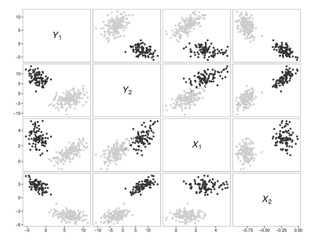
Figure 1: Scatter plots showing an example of a generated data set for Simulation 1.

One hundred samples are generated. The eMCWM family is run using all 196 models for $G\in\{1,\ldots,4\}$, resulting in a total of 784 models for each sample. Both the BIC and the ICL chose the same model each time. The VEE-VII model is chosen 91 out of 100 times. The selected model fit the correct number of components and resulted in perfect classification 99 out of 100 times (with one misclassification on the remaining sample). True and estimated parameters for the two-component VEE-VII model are reported in Table 2. Clearly, the parameter estimates are close to the true values.

Table 2: True parameter values along with mean and standard deviations of the parameter estimates (rounded off to two decimals) for the VEE-VII model from the 100 runs for Simulation 1.

Parameter	True values	Mean estimates	Standard deviations
$\pi_{1}$	0.35	0.35	0.03
$\pi_{2}$	0.65	0.65	0.03
$\boldsymbol{\mu}_{\boldsymbol{X}1}$	$(3,2.5)^{\prime}$	$(2.99,2.51)^{\prime}$	$(0.10,0.13)^{\prime}$
$\boldsymbol{\mu}_{\boldsymbol{X}2}$	$(1.1,-4)^{\prime}$	$(1.09,-4.00)^{\prime}$	$(0.05,0.05)^{\prime}$
$\lambda_{\boldsymbol{X}1}$	1	0.98	0.11
$\lambda_{\boldsymbol{X}2}$	0.5	0.50	0.04
$\boldsymbol{B}^{\prime}_{1}$	$\begin{pmatrix}2&-0.5&-1\\ -2&1.5&2\end{pmatrix}$	$\begin{pmatrix}1.97&-0.49&-1.00\\ -1.99&1.52&1.97\end{pmatrix}$	$\begin{pmatrix}0.49&0.11&0.12\\ 0.58&0.14&0.13\end{pmatrix}$
$\boldsymbol{B}^{\prime}_{2}$	$\begin{pmatrix}0&2.2&-1\\ 1&2&1.5\end{pmatrix}$	$\begin{pmatrix}-0.07&2.18&-1.02\\ 1.09&1.98&1.52\end{pmatrix}$	$\begin{pmatrix}0.68&0.15&0.15\\ 0.79&0.20&0.18\end{pmatrix}$
$\boldsymbol{\Sigma}_{\boldsymbol{Y}1}$	$\begin{pmatrix}0.92&0.56\\ 0.56&1.40\\ \end{pmatrix}$	$\begin{pmatrix}0.91&0.54\\ 0.54&1.37\\ \end{pmatrix}$	$\begin{pmatrix}0.12&0.10\\ 0.10&0.18\\ \end{pmatrix}$
$\boldsymbol{\Sigma}_{\boldsymbol{Y}2}$	$\begin{pmatrix}1.73&1.05\\ 1.05&2.63\\ \end{pmatrix}$	$\begin{pmatrix}1.67&1.00\\ 1.00&2.53\\ \end{pmatrix}$	$\begin{pmatrix}0.15&0.13\\ 0.13&0.26\\ \end{pmatrix}$

6.1.2 Simulation 2

A two-component mixture is simulated with $450$ observations with two-dimensional Gaussian responses and three-dimensional Gaussian covariates. The VVV covariance structure is used to simulate the data for both the responses and the covariates (Figure 2). The sample sizes for each group are sampled from a binomial distribution with success probability 0.40. As in Simulation 1, 100 samples are generated. The eMCWM family is again run for $G\in\{1,\ldots,4\}$. Both the BIC and the ICL chose the same model (and two components) each time. True and estimated parameters for the two-component VVV-VVV model are given in Table 3. Clearly, the parameter estimates are close on average to the true parameters. As compared to Simulation 1, where the generating model was selected by the model selection criteria in a majority of runs, more parsimonious models are usually picked here as opposed to the VVV-VVV model (which is selected only fifteen times out of one hundred). The estimated ARI values for the selected models range between 0.94 and 1.00 with a median (mean) value of 0.98 (0.98) over the 100 runs.

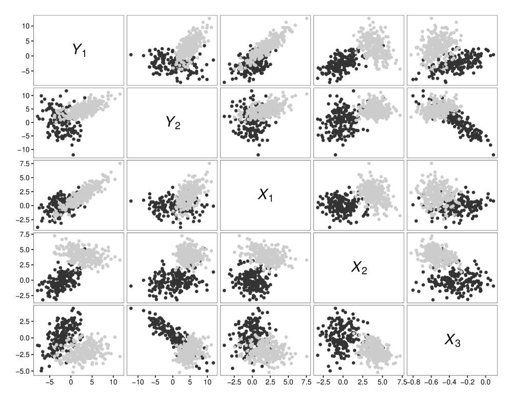
Figure 2: Scatter plots showing an example of a generated data set for Simulation 2.

Table 3: True parameter values along with mean and standard deviations of the parameter estimates (rounded off to two decimals) for the VVV-VVV model from the 100 runs for Simulation 2.

Parameter	True values	Mean estimates	Standard deviations
$\pi_{1}$	0.40	0.40	0.02
$\pi_{2}$	0.60	0.60	0.02
$\boldsymbol{\mu}_{\boldsymbol{X}1}$	$(0,0,0)^{\prime}$	$(-0.00,-0.01,-0.00)^{\prime}$	$(0.09,0.10,0.12)^{\prime}$
$\boldsymbol{\mu}_{\boldsymbol{X}2}$	$(2,4,-2)^{\prime}$	$(2.00,4.00,-2.00)^{\prime}$	$(0.09,0.05,0.06)^{\prime}$
$\boldsymbol{\Sigma}_{\boldsymbol{X}1}$	$\begin{pmatrix}1.72&-0.18&0.27\\ -0.18&1.89&0.27\\ 0.27&0.27&2.89\end{pmatrix}$	$\begin{pmatrix}1.70&-0.15&0.27\\ -0.15&1.88&0.27\\ 0.27&0.27&2.90\end{pmatrix}$	$\begin{pmatrix}0.19&0.17&0.16\\ 0.17&0.23&0.17\\ 0.16&0.17&0.29\end{pmatrix}$
$\boldsymbol{\Sigma}_{\boldsymbol{X}2}$	$\begin{pmatrix}2.33&-0.52&-0.06\\ -0.52&0.88&-0.34\\ -0.06&-0.34&1.04\end{pmatrix}$	$\begin{pmatrix}2.35&-0.52&-0.08\\ -0.52&0.88&-0.34\\ -0.08&-0.34&1.03\end{pmatrix}$	$\begin{pmatrix}0.21&0.10&0.11\\ 0.10&0.07&0.06\\ 0.11&0.06&0.09\end{pmatrix}$
$\boldsymbol{B}^{\prime}_{1}$	$\begin{pmatrix}-2&0.75&1&0.5\\ 1&0.5&1&-2\end{pmatrix}$	$\begin{pmatrix}-2.00&0.74&1.00&0.49\\ 0.99&0.49&1.00&-2.00\end{pmatrix}$	$\begin{pmatrix}0.09&0.07&0.06&0.06\\ 0.09&0.08&0.07&0.06\end{pmatrix}$
$\boldsymbol{B}^{\prime}_{2}$	$\begin{pmatrix}0.5&1.75&0.25&1\\ 1&1&1&1\end{pmatrix}$	$\begin{pmatrix}0.51&1.75&0.24&1.00\\ 1.03&1.00&1.00&1.00\end{pmatrix}$	$\begin{pmatrix}0.25&0.03&0.06&0.05\\ 0.38&0.05&0.09&0.08\end{pmatrix}$
$\boldsymbol{\Sigma}_{\boldsymbol{Y}1}$	$\begin{pmatrix}1.34&0.47\\ 0.47&1.66\\ \end{pmatrix}$	$\begin{pmatrix}1.32&0.47\\ 0.47&1.63\end{pmatrix}$	$\begin{pmatrix}0.13&0.11\\ 0.11&0.17\end{pmatrix}$
$\boldsymbol{\Sigma}_{\boldsymbol{Y}2}$	$\begin{pmatrix}0.50&0.04\\ 0.04&1.50\end{pmatrix}$	$\begin{pmatrix}0.50&0.03\\ 0.03&1.47\end{pmatrix}$	$\begin{pmatrix}0.04&0.06\\ 0.06&0.14\end{pmatrix}$

6.1.3 Simulation 3

Parameter recovery is also illustrated on higher dimensional data generated from an EEE-EEE model. One hundred samples of a two-component mixture model are simulated with nine-dimensional covariates and ten-dimensional responses. Group sample sizes are sampled from a binomial distribution with success probability 0.3 and an overall sample size of 1000. Covariates for the first component are simulated from a nine-dimensional Gaussian distribution with zero mean. Covariates for the second component are simulated with mean $(1,2,-1,-2,0,0,1,2,-1)^{\prime}$. The ten by ten matrix of regression coefficients for the two groups is simulated using a standard Gaussian distribution and fixed for all 100 runs (see Appendix C for the coefficient values). The common covariance matrix for the covariates is generated using

$$\begin{pmatrix}1.00&0.80&0.60\\ 0.80&1.20&0.40\\ 0.60&0.40&0.80\end{pmatrix}\otimes\boldsymbol{I}_{3},$$

where $\boldsymbol{I}_{3}$ denotes a 3-dimensional identity diagonal matrix. Similarly, the common covariance matrix for the responses is generated using

$$\begin{pmatrix}1.50&0.60\\ 0.60&2.00\end{pmatrix}\otimes\boldsymbol{I}_{5},$$

where $\boldsymbol{I}_{5}$ denotes a 5-dimensional identity diagonal matrix. The recovered parameter estimates for the EEE-EEE model are found to be close on average to the generating parameters. Due to space constraints and the high dimensionality, the Frobenius norms of the biases of the parameter estimates from the EEE-EEE models are reported in Table 4, similar to Murray et al. (2014).

Note that while the purpose of this simulation is to investigate parameter estimation in higher dimensions, clustering performance is also evaluated. Two-, three-, and four-component models were selected 46, 29, and 25 times, respectively. Interestingly, selection of the three- and four-component models seem to result from spurious clusters. Spurious clusters are well known in the mixture modelling literature (Ingrassia, 2004; Ingrassia and Rocci, 2007) and are commonly associated with low variance of a mixture component, leading to a spike in the log-likelihood (McLachlan and Peel, 2000; Ingrassia, 2004; Ingrassia and Rocci, 2007). In this simulation, the above is true for every run where a two-component model was not selected in the current simulation by the BIC. Such cases have been dealt with by imposing bounds on the eigenvalues of the covariance matrix of interest during parameter estimation (Ingrassia, 2004; Browne et al., 2013). This, in effect, imposes a bound on the variance along the principal axes. Here, a simple post-hoc procedure is implemented. If either of the covariates or responses covariance matrices for a model possess any eigenvalues less than a conservative bound, $\epsilon=10^{-20}$, that model is removed from the results. This procedure has the effect of disregarding all models with spurious clusters in our simulation. As a result, a two-component model is selected all 100 times; specifically, the EEE-EEE (EEE-VEE) model was selected 99 (1) times. The estimated ARI values for the selected models range between 0.996 and 1.00 with a median (mean) value of 1.00 (1.00).

Table 4: Frobenius norms of the biases of the parameter estimates (rounded off to two decimals) for the EEE-EEE model from the 100 runs for Simulation 3.

Parameter	$\|\text{Bias}\|$
$\pi_{1}$	0.00
$\pi_{2}$	0.00
$\boldsymbol{\mu}_{\boldsymbol{X}1}$	0.01
$\boldsymbol{\mu}_{\boldsymbol{X}2}$	0.01
$\boldsymbol{\Sigma}_{\boldsymbol{X}1}=\boldsymbol{\Sigma}_{\boldsymbol{X}2}$	0.03
$\boldsymbol{B}^{\prime}_{1}$	0.13
$\boldsymbol{B}^{\prime}_{2}$	0.11
$\boldsymbol{\Sigma}_{\boldsymbol{Y}1}=\boldsymbol{\Sigma}_{\boldsymbol{Y}2}$	0.12

6.2 Analysis of Real Data Sets

6.2.1 Australian Institute of Sports Data

The Australian Institute of Sports (AIS) data (Cook and Weisberg, 1994) contains measurements on 202 athletes (100 female and 102 male) and is available in the R package sn (Azzalini, 2013). A subset of seven variables that has recently been used in the mixtures of regression literature (Soffritti and Galimberti, 2011) is analyzed here: red cell count ($\mathsf{RCC}$), white cell count ($\mathsf{WCC}$), plasma ferritin concentration ($\mathsf{PFC}$), body mass index, sum of skin folds, body fat percentage, and lean body mass. The blood composition variables ($\mathsf{RCC}$, $\mathsf{WCC}$, and $\mathsf{PFC}$) are selected as the response variables with the biometrical variables being the predictors. All algorithms are run for $G\in\{1,\ldots,4\}$. Table 5 summarizes the results from running the eMCWM, eFMR, eFMRC, FMR, FMRC, and mixture GPCM algorithms.

Table 5: Comparison of the performance of the models applied to the AIS data.

Algorithm	Model	$G$	ARI	Parameters
eMCWM	VVI-VVE	2	0.92	59
eFMR	VI	1	0	18
eFMRC	VI	1	0	18
FMR		1	0	18
FMRC		1	0	18
mixture	EVE	3	0.60	63

*Note that, for a one-component model, the family comprises three covariance structures: VI (diagonal with different entries), EI (diagonal with same entries), and VV (full covariance matrix).

Both the BIC and the ICL chose a two-component model with the VVI and VVE covariance structures for the response and covariates, respectively. This model yielded an ARI of 0.92. The estimated classification for the chosen eMCWM model is in Table 6. Note that the difference between the chosen eMCWM model and the model with the second best BIC value is small ($\approx$ 0.3 BIC points). This latter model (VEI-VVE; 57 degrees of freedom) picked two components and resulted in an ARI of 0.87. The chosen (one-component) model from the eFMR and eFMRC families did not perform well, and neither did the FMR and FMRC models. The mixture software, on the other hand, selected a three-component solution but the estimated classification does not reconcile as well with the known grouping.

Table 6: Cross-tabulation of true and estimated classifications for two methods applied to the AIS data.

	eMCWM			mixture
	1	2		1	2	3
Female	99	1		83	14	3
Male	3	99		0	86	16

6.2.2 Iris Data

The algorithms are also run on the famous Iris data set (Anderson, 1935; Fisher, 1936). This data set, available in the datasets package as part of R, provides measurements on sepal length and width as well as petal length and width for 50 flowers from each of three species of Iris: setosa, versicolor, and virginica. The width measurements are taken to be the response variables with the other variables as the covariates. The algorithms are run for $G\in\{1,\ldots,4\}$ (Table 7). The selected eMCWM model is a three-component model with an ARI of 0.90 (Table 8). Note that the difference between the chosen eMCWM model and the model with the second best BIC value is $\approx$ 1.25 BIC points. This latter model selected a two-component model (VVV-VVV; 29 degrees of freedom) with an ARI of 0.57. This model put datapoints from versicolor and virginica together in one group. The model with the second best BIC value is the model that the ICL chose: a two-component VVV model with an ARI of 0.57.

Table 7: Comparison of the performance of the models applied to the Iris data.

Algorithm	Model	$G$	ARI	Parameters
eMCWM	VEV-VEV	3	0.90	40
eFMR	VEI	2	0.14	16
eFMRC	VVI	2	0.45	19
FMR		2	0.19	17
FMRC		2	0.45	19
mixture	VEV	2	0.57	26

The eFMR and FMR models resulted in two-component models yielding poor ARI values. A two-component VVI model is selected from the eFMRC family with an ARI of 0.45. This model clusters setosa and virginica perfectly with observations from versicolor assigned to the other two clusters. Because the flexmix FMRC algorithm is, in essence, a VVI model, unsurprisingly, it also chose a two-component model with an ARI of 0.45. The GPCM family as implemented in mixture picked a two-component model (ARI=0.57) with the data points from versicolor and virginica pooled together in one group (Table 8).

Table 8: Cross-tabulation of true and estimated classifications for three methods applied to the Iris data.

	eMCWM				mixture			eFMRC
	1	2	3		1	2		1	2
setosa	50				50			50
versicolor		45	5			50		31	19
virginica			50			50			50

6.2.3 Crabs Data

The crabs data set contains five morphological measurements on each of 50 crabs representing both sexes and colours (blue and orange) of the species Leptograpsus variegatus. These data were originally introduced in Campbell and Mahon (1974) and are available as part of the MASS package (Venables and Ripley, 2002) for R. The data are famous for having highly correlated measurements on width of frontal region just anterior to frontal tebercles ($\mathsf{FL}$), width of posterior region ($\mathsf{RW}$), carapace length ($\mathsf{CL}$), carapace width ($\mathsf{CW}$), and body depth ($\mathsf{BD}$). The variables $\mathsf{CW}$, $\mathsf{FL}$, and $\mathsf{RW}$ reflect width measurements and are taken to be the response variables, with $\mathsf{CL}$ and $\mathsf{BD}$ as the predictor variables. Based on the two binary variables, sex and colour, there are four known classes within these data. The algorithms are run for $G\in\{1,\ldots,9\}$ and the results are summarized in Table 9. The selected eMCWM model is a four-component model with an ARI of 0.82 (Table 10). Note that the difference between the chosen eMCWM model and the model with the second best BIC value is $\approx$ 0.6 BIC points. This latter model (EEE-EEE; 56 degrees of freedom) also picked a four-component model, with an ARI of 0.84.

Table 9: Comparison of the performance of the models applied to the crabs data.

Algorithm	Model	$G$	ARI	Parameters
eMCWM	EEE-EVE	4	0.82	59
eFMR	VVI	2	0.40	25
eFMRC	EEE	4	0.83	51
FMR		2	0.40	25
FMRC		3	0.69	42
mixture	EEV	4	0.78	68

The chosen eFMR model is a two-component VVI model with an ARI of 0.40. Because the VVI model assumes independence between the response variables, it is equivalent to the flexmix FMR model; thus, unsurprisingly, the chosen FMR model is a two-component model with an ARI of 0.40 (Table 10). Note that the estimated classification from the selected two-component eFMR model leads to good separation between the sexes of the crabs. If the class membership agreement is estimated based only on the sexes of the crabs, an ARI of 0.81 is achieved. The selected FMRC model fit three components (Table 10) with an ARI of 0.69. It basically pools together the blue males and blue females while putting the orange males and females in different clusters. eFMRC picked a four-component model with an ARI of 0.83. mixture picked a four-component model (Table 10) with an ARI of 0.78. Note that, even though the ARIs achieved from the selected eMCWM, eFMRC, and mixture models are close, the mixture model estimates more parameters than the models that utilize linear dependencies between variables. Also, note that the performance of the eFMRC model should not be surprising. Recall that, in an FMRC model, $\pi_{g}(\boldsymbol{x})$ are modelled by a multinomial logit model (DeSarbo and Cron, 1988). Anderson (1972) noted that this multinomial condition is satisfied if the covariate densities $p(\boldsymbol{x})$ are assumed to be multivariate Gaussian with the same covariance matrices, i.e., the EEE model for the covariates (cf. Ingrassia et al., 2012). Hence, the eFMRC EEE model should give similar clustering results to the eMCWM EEE-EEE model. As pointed out above, these four-component models yield ARI values of 0.83 and 0.84, respectively.

Table 10: Cross-tabulation of true and estimated classifications for four methods applied to the crabs data.

	eMCWM					eFMRC					mixture					eFMR
	1	2	3	4		1	2	3	4		1	2	3	4		1	2
BM	39	11				39	11				38	12				46	4
BF		50					50					49		1		4	46
OM			50					50					50			50
OF			4	46				3	47				5	45		2	48

“B”, “O”, “M”, and “F” refer to blue, orange, male, and female, respectively.

7 Discussion

A novel family of cluster-weighted models called the eMCWM family is presented. These models can account for heterogeneous regression data with multivariate correlated responses. The distribution of the covariates is also explicitly incorporated in the likelihood, which to the authors’ knowledge is also novel in multivariate response regression methodologies. This allows for separate imposition of an eigen-decomposed structure on the component covariance matrices of both the responses and the covariates. Hence, eMCWM can handle data where $\boldsymbol{X}$ and $\boldsymbol{Y}|\boldsymbol{x}$ might have different covariance structures. For this family, identification conditions are also provided.

The eMCWM family is parsimonious. Note that the completely unconstrained GPCM model (VVV) fits the same number of parameters as the completely unconstrained eMCWM model (VVV-VVV). The family’s performance is investigated on simulated and real benchmark data, where the BIC and the ICL are in agreement with each other for all but the iris data. More generally, the eMCWM performed better in comparison to the FMR and FMRC models because it explicitly uses the distribution of the covariates. Not using that information led to estimated clusters (from the eFMR and eFMRC as well as the flexmix FMR and FMRC models) that did not agree with the observed grouping of the data. In comparison to the GPCMs, taking into account the regression structure by use of linear dependencies aided in better clustering performance on some benchmark data sets. As implemented in flexmix, FMR only models the distribution of the (assumed independent) $\boldsymbol{Y}|\boldsymbol{x}$, while FMRC models both the distribution of (assumed independent) $\boldsymbol{Y}|\boldsymbol{x}$ and a logistic model of the covariates, respectively. GPCMs and their analogues for other distributions (e.g., Andrews and McNicholas, 2012; Punzo and McNicholas, 2015; Vrbik and McNicholas, 2014; Dang et al., 2015) do not account for linear dependencies and rely on modelling the data directly with an appropriate distribution. However, the eMCWM family models both linear dependencies and the distribution of the covariates. This results in better clustering performance when a clear regression relationship exists between the variables. Numerically, the EM algorithm is stable. However, to prevent fitting small components with low generalized variance (determinant of the covariance matrix) for the eMCWM family, the component sizes are computed before each M-step and a preset minimum size of the clusters is used (cf. McLachlan and Peel, 2000; Celeux and Diebolt, 1988; Grün and Leisch, 2008).

The framework presented lends itself to a straightforward extension to model-based classification (e.g., McNicholas, 2010; Andrews et al., 2011) and discriminant analysis (Hastie and Tibshirani, 1996). In the case of the eMCWM family, each response variable is currently regressed individually on a common set of predictor variables. This can be extended to take advantage of correlations between the response variables to improve predictive accuracy, in the fashion of the ‘curds and whey’ method (Breiman and Friedman, 1997). Here, the Gaussian distribution is used for both the distribution of the covariates and the response for the eMCWM family. For heavier tailed data, mixtures of more robust distributions, such as the multivariate $t$ distribution (Andrews and McNicholas, 2012) or the multivariate power exponential distribution (that can also model lighter tailed data) (Dang et al., 2015) may be employed. The use of continuous distributions may be restrictive and more work needs to be done to incorporate mixed type data for both responses and covariates (see Punzo and Ingrassia, 2015, for the univariate case $d=p=1$).

Conflict of Interest

The authors have declared no conflict of interest.

Appendix

Appendix A Proof of Theorem 1

Proof.

The proof builds upon results given in Hennig (2000) and Ingrassia et al. (2015). Consider the class of models defined in (3). The equality

$$\sum^{G}_{g=1}\phi_{d}(\boldsymbol{y}|\boldsymbol{x},\boldsymbol{\mu}_{\boldsymbol{Y}}(\boldsymbol{x}|\boldsymbol{B}_{g}),\boldsymbol{\Sigma}_{\boldsymbol{Y}g})\phi_{p}(\boldsymbol{x}|\boldsymbol{\mu}_{\boldsymbol{X}g},\boldsymbol{\Sigma}_{\boldsymbol{X}g})\pi_{g}=\sum^{\widetilde{G}}_{s=1}\phi_{d}(\boldsymbol{y}|\boldsymbol{x},\boldsymbol{\mu}_{\boldsymbol{Y}}(\boldsymbol{x}|\widetilde{\boldsymbol{B}}_{s}),\widetilde{\boldsymbol{\Sigma}}_{\boldsymbol{Y}s})\phi_{p}(\boldsymbol{x}|\widetilde{\boldsymbol{\mu}}_{\boldsymbol{X}s},\widetilde{\boldsymbol{\Sigma}}_{\boldsymbol{X}s})\widetilde{\pi}_{s}$$ (10)

will be proven to hold for almost all $\boldsymbol{x}\in\mathbb{R}^{p}$ and for all $\boldsymbol{y}\in\mathbb{R}^{d}$ if and only if $G=\widetilde{G}$, and for each $g\in\{1,\ldots,G\}$, there exists $s\in\{1,\ldots,G\}$ such that $\boldsymbol{B}_{g}=\widetilde{\boldsymbol{B}}_{s}$, $\boldsymbol{\mu}_{\boldsymbol{X}g}=\widetilde{\boldsymbol{\mu}}_{\boldsymbol{X}s}$, $\boldsymbol{\Sigma}_{\boldsymbol{X}g}=\widetilde{\boldsymbol{\Sigma}}_{\boldsymbol{X}s}$, $\boldsymbol{\mu}_{\boldsymbol{Y}g}=\widetilde{\boldsymbol{\mu}}_{\boldsymbol{Y}s}$, $\boldsymbol{\Sigma}_{\boldsymbol{Y}g}=\widetilde{\boldsymbol{\Sigma}}_{\boldsymbol{Y}s}$, and $\pi_{g}=\widetilde{\pi}_{s}$.

Integrating each side of (10) over $\mathbb{R}^{d}$ yields

$$\sum^{G}_{g=1}\phi_{p}(\boldsymbol{x}|\boldsymbol{\mu}_{\boldsymbol{X}g},\boldsymbol{\Sigma}_{\boldsymbol{X}g})\pi_{g}=\sum^{\widetilde{G}}_{s=1}\phi_{p}(\boldsymbol{x}|\widetilde{\boldsymbol{\mu}}_{\boldsymbol{X}s},\widetilde{\boldsymbol{\Sigma}}_{\boldsymbol{X}s})\widetilde{\pi}_{s}.$$ (11)

Let

$$p(\boldsymbol{x}|\boldsymbol{\mu}_{\boldsymbol{X}},\boldsymbol{\Sigma}_{\boldsymbol{X}},\boldsymbol{\pi})=\sum^{G}_{g=1}\phi_{p}(\boldsymbol{x}|\boldsymbol{\mu}_{\boldsymbol{X}g},\boldsymbol{\Sigma}_{\boldsymbol{X}g})\pi_{g}$$

and

$$p(\boldsymbol{x}|\widetilde{\boldsymbol{\mu}}_{\boldsymbol{X}},\widetilde{\boldsymbol{\Sigma}}_{\boldsymbol{X}},\widetilde{\boldsymbol{\pi}})=\sum^{\widetilde{G}}_{s=1}\phi_{p}(\boldsymbol{x}|\widetilde{\boldsymbol{\mu}}_{\boldsymbol{X}s},\widetilde{\boldsymbol{\Sigma}}_{\boldsymbol{X}s})\widetilde{\pi}_{s},$$

where $\boldsymbol{\mu}_{\boldsymbol{X}}=\left\{\boldsymbol{\mu}_{\boldsymbol{X}g};\,g=1,\ldots,G\right\}$, $\boldsymbol{\Sigma}_{\boldsymbol{X}}=\left\{\boldsymbol{\Sigma}_{\boldsymbol{X}g};\,g=1,\ldots,G\right\}$, and $\boldsymbol{\pi}=\{\pi_{g};\,g=1,\ldots,G\}$. Analogous notation applies for $\widetilde{\boldsymbol{\mu}}_{\boldsymbol{X}},\widetilde{\boldsymbol{\Sigma}}_{\boldsymbol{X}}$, and $\widetilde{\boldsymbol{\pi}}$. Based on Bayes’ theorem,

$$p(\Omega_{g}|\boldsymbol{x},\boldsymbol{\mu}_{\boldsymbol{X}},\boldsymbol{\Sigma}_{\boldsymbol{X}},\boldsymbol{\pi})=\frac{\phi_{p}(\boldsymbol{x}|\boldsymbol{\mu}_{\boldsymbol{X}g},\boldsymbol{\Sigma}_{\boldsymbol{X}g})\pi_{g}}{p(\boldsymbol{x}|\boldsymbol{\mu}_{\boldsymbol{X}},\boldsymbol{\Sigma}_{\boldsymbol{X}},\boldsymbol{\pi})},$$ (12)

for $g=1,\ldots,G$. Then, model (2) can be rewritten as

$$p(\boldsymbol{x},\boldsymbol{y}|\boldsymbol{\vartheta}) =p(\boldsymbol{x}|\boldsymbol{\mu}_{\boldsymbol{X}},\boldsymbol{\Sigma}_{\boldsymbol{X}},\boldsymbol{\pi})\sum^{G}_{g=1}\phi_{d}(\boldsymbol{y}|\boldsymbol{x},\boldsymbol{\mu}_{\boldsymbol{Y}}(\boldsymbol{x}|\boldsymbol{B}_{g}),\boldsymbol{\Sigma}_{\boldsymbol{Y}g})p(\Omega_{g}|\boldsymbol{x},\boldsymbol{\mu}_{\boldsymbol{X}},\boldsymbol{\Sigma}_{\boldsymbol{X}},\boldsymbol{\pi})$$

$$=p(\boldsymbol{x}|\boldsymbol{\mu}_{\boldsymbol{X}},\boldsymbol{\Sigma}_{\boldsymbol{X}},\boldsymbol{\pi})p(\boldsymbol{y}|\boldsymbol{x},\boldsymbol{\vartheta}),$$ (13)

where

$$p(\boldsymbol{y}|\boldsymbol{x},\boldsymbol{\vartheta})=\sum^{G}_{g=1}\phi_{d}(\boldsymbol{y}|\boldsymbol{x},\boldsymbol{\mu}_{\boldsymbol{Y}}(\boldsymbol{x}|\boldsymbol{B}_{g}),\boldsymbol{\Sigma}_{\boldsymbol{Y}g})p(\Omega_{g}|\boldsymbol{x},\boldsymbol{\mu}_{\boldsymbol{X}},\boldsymbol{\Sigma}_{\boldsymbol{X}},\boldsymbol{\pi}),\quad\boldsymbol{y}\in\mathbb{R}^{d}.$$ (14)

Now, the class of models defined by (14) for almost all $\boldsymbol{x}\in\mathbb{R}^{p}$, if the equality

$$\sum^{G}_{g=1}\phi_{d}(\boldsymbol{y}|\boldsymbol{x},\boldsymbol{\mu}_{\boldsymbol{Y}}(\boldsymbol{x}|\boldsymbol{B}_{g}),\boldsymbol{\Sigma}_{\boldsymbol{Y}g})p(\Omega_{g}|\boldsymbol{x},\boldsymbol{\mu}_{\boldsymbol{X}},\boldsymbol{\Sigma}_{\boldsymbol{X}},\boldsymbol{\pi})=\sum^{\widetilde{G}}_{s=1}\phi_{d}(\boldsymbol{y}|\boldsymbol{x},\boldsymbol{\mu}_{\boldsymbol{Y}}(\boldsymbol{x}|\widetilde{\boldsymbol{B}}_{s}),\widetilde{\boldsymbol{\Sigma}}_{\boldsymbol{Y}s})p(\Omega_{s}|\boldsymbol{x},\widetilde{\boldsymbol{\mu}}_{\boldsymbol{X}},\widetilde{\boldsymbol{\Sigma}}_{\boldsymbol{X}},\widetilde{\boldsymbol{\pi}})$$

implies $G=\widetilde{G}$, and for each $g\in\{1,\ldots,G\}$, there exists $s\in\{1,\ldots,G\}$ such that $\boldsymbol{B}_{g}=\widetilde{\boldsymbol{B}}_{s}$, $\boldsymbol{\Sigma}_{\boldsymbol{Y}g}=\widetilde{\boldsymbol{\Sigma}}_{\boldsymbol{Y}s}$, $\boldsymbol{\mu}_{\boldsymbol{X}g}=\widetilde{\boldsymbol{\mu}}_{\boldsymbol{X}s}$, $\boldsymbol{\Sigma}_{\boldsymbol{X}g}=\widetilde{\boldsymbol{\Sigma}}_{\boldsymbol{X}s}$, and $\pi_{g}=\widetilde{\pi}_{s}$.

Recall from Section 2 that the expected value $\boldsymbol{\mu}_{\boldsymbol{Y}}$ of $Y|\Omega_{g}$ is related to the covariates $\boldsymbol{X}$ through the relation $\boldsymbol{\mu}_{\boldsymbol{Y}}=\boldsymbol{B}^{\prime}_{g}\boldsymbol{x}^{*}$, $g=1,\ldots,G$. Let

$$\mathcal{X} =\Bigl{\{}\boldsymbol{x}\in\mathbb{R}^{p}:\mbox{ for each }g,j\in\{1,\ldots,G\},\text{ and }s,t\in\{1,\ldots,\widetilde{G}\}:\Bigr{.}$$

$$\qquad\Bigl{.}\boldsymbol{B}^{\prime}_{g}\boldsymbol{x}^{*}=\boldsymbol{B}^{\prime}_{j}\boldsymbol{x}^{*}\ \Rightarrow\ \boldsymbol{B}_{g}=\boldsymbol{B}_{j},\Bigr{.}$$

$$\qquad\Bigl{.}\boldsymbol{B}^{\prime}_{g}\boldsymbol{x}^{*}=\widetilde{\boldsymbol{B}}^{\prime}_{s}\boldsymbol{x}^{*}\ \Rightarrow\ \boldsymbol{B}_{g}=\widetilde{\boldsymbol{B}}_{s},\Bigr{.}$$

$$\qquad\Bigl{.}\widetilde{\boldsymbol{B}}^{\prime}_{s}\boldsymbol{x}^{*}=\widetilde{\boldsymbol{B}}^{\prime}_{t}\boldsymbol{x}^{*}\ \Rightarrow\ \widetilde{\boldsymbol{B}}_{s}=\widetilde{\boldsymbol{B}}_{t}\Bigr{\}}.$$

According to (3), $(\boldsymbol{B}_{g},\boldsymbol{\Sigma}_{\boldsymbol{Y}g})\neq(\boldsymbol{B}_{j},\boldsymbol{\Sigma}_{\boldsymbol{Y}j})$, $g\neq j$; thus, it follows that the quantities $(\boldsymbol{B}^{\prime}_{g}\boldsymbol{x}^{*},\boldsymbol{\Sigma}_{\boldsymbol{Y}g})$, $g=1,\ldots,G$, are pairwise distinct for all $\boldsymbol{x}\in\mathcal{X}$ (indeed, the complement of $\mathcal{X}$, i.e., $\mathbb{R}^{p}\setminus\mathcal{X}$, is formed by a finite set of hyperplanes of $\mathbb{R}^{p}$ and, thus, $\mathbb{R}^{p}\setminus\mathcal{X}$ has null measure).

For any fixed $\boldsymbol{x}\in\mathcal{X}$, according to (12), $\{p(\Omega_{1}|\boldsymbol{x},\boldsymbol{\mu}_{\boldsymbol{X}},\boldsymbol{\Sigma}_{\boldsymbol{X}},\boldsymbol{\pi}),\ldots,p(\Omega_{G}|\boldsymbol{x},\boldsymbol{\mu}_{\boldsymbol{X}},\boldsymbol{\Sigma}_{\boldsymbol{X}},\boldsymbol{\pi})\}$ and $\{p(\Omega_{1}|\boldsymbol{x},\widetilde{\boldsymbol{\mu}}_{\boldsymbol{X}},\widetilde{\boldsymbol{\Sigma}}_{\boldsymbol{X}},\widetilde{\boldsymbol{\pi}}),\ldots,p(\Omega_{\widetilde{G}}|\boldsymbol{x},\widetilde{\boldsymbol{\mu}}_{\boldsymbol{X}},\widetilde{\boldsymbol{\Sigma}}_{\boldsymbol{X}},\widetilde{\boldsymbol{\pi}})\}$ are sets of positive numbers summing to one. It follows that, for each $\boldsymbol{x}\in\mathcal{X}$, the density $p(\boldsymbol{y}|\boldsymbol{x},\boldsymbol{\vartheta})$ given in (14) is a mixture of distributions of kind (4) and then it is identifiable, due to the assumptions of the theorem. Thus, $G=\widetilde{G}$ and there exists $s\in\{1,\ldots,G\}$ such that

$$\boldsymbol{B}_{g}=\widetilde{\boldsymbol{B}}_{s},\quad\boldsymbol{\Sigma}_{\boldsymbol{Y}g}=\widetilde{\boldsymbol{\Sigma}}_{\boldsymbol{Y}s}\quad\text{and}\quad p(\Omega_{g}|\boldsymbol{x},\boldsymbol{\mu}_{\boldsymbol{X}},\boldsymbol{\Sigma}_{\boldsymbol{X}},\boldsymbol{\pi})=p(\Omega_{s}|\boldsymbol{x},\widetilde{\boldsymbol{\mu}}_{\boldsymbol{X}},\widetilde{\boldsymbol{\Sigma}}_{\boldsymbol{X}},\widetilde{\boldsymbol{\pi}}).$$ (15)

Moreover, because $p(\Omega_{g}|\boldsymbol{x},\boldsymbol{\mu}_{\boldsymbol{X}},\boldsymbol{\Sigma}_{\boldsymbol{X}},\boldsymbol{\pi})$ and $p(\Omega_{s}|\boldsymbol{x},\widetilde{\boldsymbol{\mu}}_{\boldsymbol{X}},\widetilde{\boldsymbol{\Sigma}}_{\boldsymbol{X}},\widetilde{\boldsymbol{\pi}})$ are defined according to (12), from (15) and (11), we get:

$$\pi_{g} =\int_{\mathcal{X}}\pi_{g}\phi_{p}(\boldsymbol{x}|\boldsymbol{\mu}_{\boldsymbol{X}g},\boldsymbol{\Sigma}_{\boldsymbol{X}g})d\boldsymbol{x}$$

$$=\int_{\mathcal{X}}\frac{\pi_{g}\phi_{p}(\boldsymbol{x}|\boldsymbol{\mu}_{\boldsymbol{X}g},\boldsymbol{\Sigma}_{\boldsymbol{X}g})}{\sum^{G}_{g=1}\phi_{p}(\boldsymbol{x}|\boldsymbol{\mu}_{\boldsymbol{X}g},\boldsymbol{\Sigma}_{\boldsymbol{X}g})\pi_{g}}\left(\sum^{G}_{g=1}\phi_{p}(\boldsymbol{x}|\boldsymbol{\mu}_{\boldsymbol{X}g},\boldsymbol{\Sigma}_{\boldsymbol{X}g})\pi_{g}\right)d\boldsymbol{x}$$

$$=\int_{\mathcal{X}}p(\Omega_{g}|\boldsymbol{x},\boldsymbol{\mu}_{\boldsymbol{X}},\boldsymbol{\Sigma}_{\boldsymbol{X}},\boldsymbol{\pi})\left(\sum^{\widetilde{G}}_{s=1}\phi_{p}(\boldsymbol{x}|\widetilde{\boldsymbol{\mu}}_{\boldsymbol{X}s},\widetilde{\boldsymbol{\Sigma}}_{s})\widetilde{\pi}_{s}\right)d\boldsymbol{x}$$

$$=\int_{\mathcal{X}}p(\Omega_{s}|\boldsymbol{x},\boldsymbol{\mu}_{\boldsymbol{X}},\boldsymbol{\Sigma}_{\boldsymbol{X}},\boldsymbol{\pi})\left(\sum^{\widetilde{G}}_{s=1}\phi_{p}(\boldsymbol{x}|\widetilde{\boldsymbol{\mu}}_{\boldsymbol{X}s},\widetilde{\boldsymbol{\Sigma}}_{\boldsymbol{X}s})\widetilde{\pi}_{s}\right)d\boldsymbol{x}$$

$$=\int_{\mathcal{X}}\frac{\widetilde{\pi}_{s}\phi_{p}(\boldsymbol{x}|\widetilde{\boldsymbol{\mu}}_{\boldsymbol{X}s},\widetilde{\boldsymbol{\Sigma}}_{\boldsymbol{X}s})}{\sum^{\widetilde{G}}_{t=1}\phi_{p}(\boldsymbol{x}|\widetilde{\boldsymbol{\mu}}_{\boldsymbol{X}t},\widetilde{\boldsymbol{\Sigma}}_{\boldsymbol{X}t})\widetilde{\pi}_{t}}\left(\sum^{\widetilde{G}}_{s=1}\phi_{p}(\boldsymbol{x}|\widetilde{\boldsymbol{\mu}}_{\boldsymbol{X}s},\widetilde{\boldsymbol{\Sigma}}_{\boldsymbol{X}s})\widetilde{\pi}_{s}\right)d\boldsymbol{x}$$

$$=\int_{\mathcal{X}}\widetilde{\pi}_{s}\phi_{p}(\boldsymbol{x}|\widetilde{\boldsymbol{\mu}}_{\boldsymbol{X}s},\widetilde{\boldsymbol{\Sigma}}_{\boldsymbol{X}s})d\boldsymbol{x}=\widetilde{\pi}_{s}.$$

Moreover,

$$\phi_{p}(\boldsymbol{x}|\boldsymbol{\mu}_{\boldsymbol{X}g},\boldsymbol{\Sigma}_{g}) =\frac{p(\Omega_{g}|\boldsymbol{x},\boldsymbol{\mu}_{\boldsymbol{X}g},\boldsymbol{\Sigma}_{\boldsymbol{X}g},\boldsymbol{\pi})}{\pi_{g}}\sum^{G}_{g=1}\phi_{p}(\boldsymbol{x}|\boldsymbol{\mu}_{\boldsymbol{X}g},\boldsymbol{\Sigma}_{\boldsymbol{X}g})\pi_{g}$$

$$=\frac{p(\Omega_{s}|\boldsymbol{x},\widetilde{\boldsymbol{\mu}}_{\boldsymbol{X}},\widetilde{\boldsymbol{\Sigma}}_{\boldsymbol{X}},\widetilde{\boldsymbol{\pi}})}{\widetilde{\pi}_{s}}\sum^{\widetilde{G}}_{s=1}\phi_{p}(\boldsymbol{x}|\widetilde{\boldsymbol{\mu}}_{\boldsymbol{X}s},\widetilde{\boldsymbol{\Sigma}}_{\boldsymbol{X}s})\widetilde{\pi}_{s}=\phi_{p}(\boldsymbol{x}|\widetilde{\boldsymbol{\mu}}_{\boldsymbol{X}s},\widetilde{\boldsymbol{\Sigma}}_{\boldsymbol{X}s}).$$

From the identifiability of Gaussian distributions, again for the same pair $(g,s)$ in (15), it follows that

$$\quad\boldsymbol{\mu}_{\boldsymbol{X}g}=\widetilde{\boldsymbol{\mu}}_{\boldsymbol{X}s}\quad\text{and}\quad\boldsymbol{\Sigma}_{\boldsymbol{X}g}=\widetilde{\boldsymbol{\Sigma}}_{\boldsymbol{X}s},$$

and this completes the proof. ∎

Appendix B M-step

Derivation of $\hat{\boldsymbol{B}}_{g}^{(k+1)}$:

For the estimate of the regression coefficients $\hat{\boldsymbol{B}}_{g}^{(k+1)}$, $g=1,\ldots,G$:

$$\sum_{i=1}^{N}\sum_{g=1}^{G}\hat{z}_{ig}^{(k)}\frac{\partial Q_{1}\left(\boldsymbol{B}_{g},\boldsymbol{\Sigma}_{\boldsymbol{Y}g}|\boldsymbol{\vartheta}^{(k)}\right)}{\partial\boldsymbol{B}^{\prime}_{g}}=\boldsymbol{0}^{\prime},$$

which implies

$$\frac{\partial\left\{\displaystyle\sum_{i=1}^{N}\sum_{g=1}^{G}\frac{-\hat{z}_{ig}^{(k)}}{2}\left[\left(\boldsymbol{y}_{i}-\boldsymbol{B}^{\prime}_{g}\boldsymbol{x}_{i}^{*}\right)^{\prime}\boldsymbol{\Sigma}_{\boldsymbol{Y}g}^{-1}\left(\boldsymbol{y}_{i}-\boldsymbol{B}^{\prime}_{g}\boldsymbol{x}_{i}^{*}\right)\right]\right\}}{\partial\boldsymbol{B}^{\prime}_{g}}=\boldsymbol{0}^{\prime},$$

yielding

$$\frac{\partial\left[\displaystyle\sum_{i=1}^{N}\sum_{g=1}^{G}\frac{-\hat{z}_{ig}^{(k)}}{2}\left(-\boldsymbol{y}^{\prime}_{i}\boldsymbol{\Sigma}_{\boldsymbol{Y}g}^{-1}\boldsymbol{B}^{\prime}_{g}\boldsymbol{x}_{i}^{*}-\boldsymbol{x}_{i}^{*^{\prime}}\boldsymbol{B}_{g}\boldsymbol{\Sigma}_{\boldsymbol{Y}g}^{-1}\boldsymbol{y}_{i}+\boldsymbol{x}_{i}^{*^{\prime}}\boldsymbol{B}_{g}\boldsymbol{\Sigma}_{\boldsymbol{Y}g}^{-1}\boldsymbol{B}^{\prime}_{g}\boldsymbol{x}_{i}^{*}\right)\right]}{\partial\boldsymbol{B}^{\prime}_{g}}=\boldsymbol{0}^{\prime}.$$

Using properties of trace and transpose, we get

$$\frac{\partial\left\{\displaystyle\sum_{i=1}^{N}\sum_{g=1}^{G}\frac{\hat{z}_{ig}^{(k)}}{2}\left[\mbox{tr}\left(\boldsymbol{y}^{\prime}_{i}\boldsymbol{\Sigma}_{\boldsymbol{Y}g}^{-1}\boldsymbol{B}^{\prime}_{g}\boldsymbol{x}_{i}^{*}\right)+\mbox{tr}\left(\boldsymbol{x}_{i}^{*^{\prime}}\boldsymbol{B}_{g}\boldsymbol{\Sigma}_{\boldsymbol{Y}g}^{-1}\boldsymbol{y}_{i}\right)-\mbox{tr}\left(\boldsymbol{x}_{i}^{*^{\prime}}\boldsymbol{B}_{g}\boldsymbol{\Sigma}_{\boldsymbol{Y}g}^{-1}\boldsymbol{B}^{\prime}_{g}\boldsymbol{x}_{i}^{*}\right)\right]\right\}}{\partial\boldsymbol{B}^{\prime}_{g}} =\boldsymbol{0}^{\prime}$$

$$\frac{\partial\left\{\displaystyle\sum_{i=1}^{N}\sum_{g=1}^{G}\frac{\hat{z}_{ig}^{(k)}}{2}\left[\mbox{tr}\left(\boldsymbol{B}^{\prime}_{g}\boldsymbol{x}_{i}^{*}\boldsymbol{y}^{\prime}_{i}\boldsymbol{\Sigma}_{\boldsymbol{Y}g}^{-1}\right)+\mbox{tr}\left(\left(\boldsymbol{\Sigma}_{\boldsymbol{Y}g}^{-1}\boldsymbol{y}_{i}\boldsymbol{x}_{i}^{*^{\prime}}\right)^{\prime}\boldsymbol{B}^{\prime}_{g}\right)-\mbox{tr}\left(\boldsymbol{B}^{\prime}_{g}\boldsymbol{x}_{i}^{*}\boldsymbol{x}_{i}^{*^{\prime}}\boldsymbol{B}_{g}\boldsymbol{\Sigma}_{\boldsymbol{Y}g}^{-1}\right)\right]\right\}}{\partial\boldsymbol{B}^{\prime}_{g}} =\boldsymbol{0}^{\prime}.$$

Taking the derivative, we obtain

$$\sum_{i=1}^{N}\frac{\hat{z}_{ig}^{(k)}}{2}\left\{\boldsymbol{\Sigma}_{\boldsymbol{Y}g}^{-1}\boldsymbol{y}_{i}\boldsymbol{x}_{i}^{*^{\prime}}+\boldsymbol{\Sigma}_{\boldsymbol{Y}g}^{-1}\boldsymbol{y}_{i}\boldsymbol{x}_{i}^{*^{\prime}}-\left[\left(\boldsymbol{\Sigma}_{\boldsymbol{Y}g}^{-1}\right)^{\prime}\boldsymbol{B}^{\prime}_{g}\boldsymbol{x}_{i}^{*}\boldsymbol{x}_{i}^{*^{\prime}}+\boldsymbol{\Sigma}_{\boldsymbol{Y}g}^{-1}\boldsymbol{B}^{\prime}_{g}\boldsymbol{x}_{i}^{*}\boldsymbol{x}_{i}^{*^{\prime}}\right]\right\} =\boldsymbol{0}^{\prime},$$

and finally

$$\hat{\boldsymbol{B}}_{g}^{(k+1)^{\prime}} =\left(\sum_{i=1}^{N}\hat{z}_{ig}^{(k)}\boldsymbol{y}_{i}\boldsymbol{x}_{i}^{*^{\prime}}\right)\left({\sum_{i=1}^{N}\hat{z}_{ig}^{(k)}\boldsymbol{x}_{i}^{*}\boldsymbol{x}_{i}^{*^{\prime}}}\right)^{-1}.$$

Derivation of $\hat{\boldsymbol{\Sigma}}_{\boldsymbol{Y}g}^{(k+1)}$:

For the estimate of the covariance matrix $\hat{\boldsymbol{\Sigma}}_{\boldsymbol{Y}g}^{(k+1)}$, $g=1,\ldots,G$:

$$\sum_{i=1}^{N}\hat{z}_{ig}^{(k)}\frac{\partial Q_{1}\left(\boldsymbol{B}^{(k+1)}_{g},\boldsymbol{\Sigma}_{\boldsymbol{Y}g}|\boldsymbol{\vartheta}^{(k)}\right)}{\partial\boldsymbol{\Sigma}^{-1}_{\boldsymbol{Y}g}}=\boldsymbol{0}^{\prime},$$

leading to

$$\frac{\partial\left\{\displaystyle\sum_{i=1}^{N}\sum_{g=1}^{G}\frac{\hat{z}_{ig}^{(k)}}{2}\left[\log|\boldsymbol{\Sigma}_{\boldsymbol{Y}g}^{-1}|-\mbox{tr}\left(\left(\boldsymbol{y}_{i}-\boldsymbol{B}^{(k+1)^{\prime}}_{g}\boldsymbol{x}_{i}^{*}\right)^{\prime}\boldsymbol{\Sigma}_{\boldsymbol{Y}g}^{-1}\left(\boldsymbol{y}_{i}-\boldsymbol{B}^{(k+1)^{\prime}}_{g}\boldsymbol{x}_{i}^{*}\right)\right)\right]\right\}}{\partial\boldsymbol{\Sigma}^{-1}_{\boldsymbol{Y}g}} =\boldsymbol{0}^{\prime},$$

$$\frac{\partial\left\{\displaystyle\sum_{i=1}^{N}\sum_{g=1}^{G}\frac{\hat{z}_{ig}^{(k)}}{2}\left[\log|\boldsymbol{\Sigma}_{\boldsymbol{Y}g}^{-1}|-\mbox{tr}\left(\boldsymbol{\Sigma}_{\boldsymbol{Y}g}^{-1}\left(\boldsymbol{y}_{i}-\boldsymbol{B}^{(k+1)^{\prime}}_{g}\boldsymbol{x}_{i}^{*}\right)\left(\boldsymbol{y}_{i}-\boldsymbol{B}^{(k+1)^{\prime}}_{g}\boldsymbol{x}_{i}^{*}\right)^{\prime}\right)\right]\right\}}{\partial\boldsymbol{\Sigma}^{-1}_{\boldsymbol{Y}g}} =\boldsymbol{0}^{\prime}.$$

Taking the derivative, we get

$$\sum_{i=1}^{N}\frac{\hat{z}_{ig}^{(k)}}{2}\left\{\left(\boldsymbol{\Sigma}_{\boldsymbol{Y}g}^{-1}\right)^{-1^{\prime}}-\left[\left(\boldsymbol{y}_{i}-\boldsymbol{B}^{(k+1)^{\prime}}_{g}\boldsymbol{x}_{i}^{*}\right)\left(\boldsymbol{y}_{i}-\boldsymbol{B}^{(k+1)^{\prime}}_{g}\boldsymbol{x}_{i}^{*}\right)^{\prime}\right]^{\prime}\right\}=\boldsymbol{0}^{\prime},$$

and this results in

$$\hat{\boldsymbol{\Sigma}}_{\boldsymbol{Y}g}^{(k+1)}=\frac{\displaystyle\sum_{i=1}^{N}\hat{z}_{ig}^{(k)}\left(\boldsymbol{y}_{i}-\hat{\boldsymbol{B}}_{g}^{(k+1)^{\prime}}\boldsymbol{x}_{i}^{*}\right)\left(\boldsymbol{y}_{i}-\hat{\boldsymbol{B}}_{g}^{(k+1)^{\prime}}\boldsymbol{x}_{i}^{*}\right)^{\prime}}{\displaystyle\sum_{i=1}^{N}\hat{z}_{ig}^{(k)}}.$$

Appendix C Regression Coefficients for Simulation 3

Regression coefficients used to generate data for group 1 for Simulation 3:

$$\begin{pmatrix}[r]-0.63&0.18&-0.84&1.60&0.33&-0.82&0.49&0.74&0.58&-0.31\\ 1.51&0.39&-0.62&-2.21&1.12&-0.04&-0.02&0.94&0.82&0.59\\ 0.92&0.78&0.07&-1.99&0.62&-0.06&-0.16&-1.47&-0.48&0.42\\ 1.36&-0.10&0.39&-0.05&-1.38&-0.41&-0.39&-0.06&1.10&0.76\\ -0.16&-0.25&0.70&0.56&-0.69&-0.71&0.36&0.77&-0.11&0.88\\ 0.40&-0.61&0.34&-1.13&1.43&1.98&-0.37&-1.04&0.57&-0.14\\ 2.40&-0.04&0.69&0.03&-0.74&0.19&-1.80&1.47&0.15&2.17\\ 0.48&-0.71&0.61&-0.93&-1.25&0.29&-0.44&0.00&0.07&-0.59\\ -0.57&-0.14&1.18&-1.52&0.59&0.33&1.06&-0.30&0.37&0.27\\ -0.54&1.21&1.16&0.70&1.59&0.56&-1.28&-0.57&-1.22&-0.47\\ \end{pmatrix}$$

Regression coefficients used to generate data for group 2 for Simulation 3:

$$\begin{pmatrix}[r]-0.62&0.04&-0.91&0.16&-0.65&1.77&0.72&0.91&0.38&1.68\\ -0.64&-0.46&1.43&-0.65&-0.21&-0.39&-0.32&-0.28&0.49&-0.18\\ -0.51&1.34&-0.21&-0.18&-0.10&0.71&-0.07&-0.04&-0.68&-0.32\\ 0.06&-0.59&0.53&-1.52&0.31&-1.54&-0.30&-0.53&-0.65&-0.06\\ -1.91&1.18&-1.66&-0.46&-1.12&-0.75&2.09&0.02&-1.29&-1.64\\ 0.45&-0.02&-0.32&-0.93&-1.49&-1.08&1.00&-0.62&-1.38&1.87\\ 0.43&-0.24&1.06&0.89&-0.62&2.21&-0.26&-1.42&-0.14&0.21\\ 2.31&0.11&0.46&-0.08&-0.33&-0.03&0.79&2.08&1.03&1.21\\ -1.23&0.98&0.22&-1.47&0.52&-0.16&1.46&-0.77&-0.43&-0.93\\ -0.18&0.40&-0.73&0.83&-1.21&-1.05&1.44&-1.02&0.41&-0.38\\ \end{pmatrix}$$

References

- Aitken (1926) Aitken, A. C. (1926). On Bernoulli’s numerical solution of algebraic equations. In Proceedings of the Royal Society of Edinburgh, volume 46, pages 289–305.
- Anderlucci and Viroli (2015) Anderlucci, L. and Viroli, C. (2015). Covariance pattern mixture models for multivariate longitudinal data. The Annals of Applied Statistics 9(2), 777–800.
- Anderson (1935) Anderson, E. (1935). The irises of the Gaspé peninsula. Bulletin of the American Iris Society, 59, 2–5.
- Anderson (1972) Anderson, J. A. (1972). Separate sample logistic discrimination. Biometrika, 59(1), 19–35.
- Andrews and McNicholas (2012) Andrews, J. L. and McNicholas, P. D. (2012). Model-based clustering, classification, and discriminant analysis via mixtures of multivariate -distributions. Statistics and Computing, 22(5), 1021–1029.
- Andrews and McNicholas (2014) Andrews, J. L. and McNicholas, P. D. (2014). Variable selection for clustering and classification. Journal of Classification 31(2), 136–153.
- Andrews et al. (2011) Andrews, J. L., McNicholas, P. D., and Subedi, S. (2011). Model-based classification via mixtures of multivariate -distributions. Computational Statistics and Data Analysis, 55(1), 520–529.
- Azzalini (2013) Azzalini, A. (2013). sn: The skew-normal and skew- distributions. R package version 0.4-18.
- Baudry and Celeux (2015) Baudry, J.-P. and Celeux, G. (2015). EM for mixtures. Statistics and Computing, 25(4), 713–726.
- Biernacki and Lourme (2014) Biernacki, C. and Lourme, A. (2014). Stable and visualizable Gaussian parsimonious clustering models. Statistics and Computing, 24(6), 953–969.
- Biernacki et al. (2000) Biernacki, C., Celeux, G., and Govaert, G. (2000). Assessing a mixture model for clustering with the integrated completed likelihood. IEEE Transactions on Pattern Analysis and Machine Intelligence, 22(7), 719–725.
- Böhning (1995) Böhning, D. (1995). A review of reliable algorithms for the semi-parametric maximum likelihood estimator of a mixture distribution. Journal of Statistical Planning and Inference, 47, 5–28.
- Böhning (2000) Böhning, D. (2000). Computer-Assisted Analysis of Mixtures and Applications: Meta-analysis, Disease Mapping and Others. Chapman & Hall/CRC, London.
- Böhning (2003) Böhning, D. (2003). The EM algorithm with gradient function update for discrete mixtures with known (fixed) number of components. Statistics and Computing, 13(3), 257–265.
- Böhning et al. (1994) Böhning, D., Dietz, E., Schaub, R., Schlattmann, P., and Lindsay, B. G. (1994). The distribution of the likelihood ratio for mixtures of densities from the one-parameter exponential family. Annals of the Institute of Statistical Mathematics, 46(2), 373–388.
- Bouveyron and Brunet-Saumard (2014) Bouveyron, C. and Brunet-Saumard, C. (2014). Model-based clustering of high-dimensional data: A review. Computational Statistics and Data Analysis, 71, 52–78.
- Breiman and Friedman (1997) Breiman, L. and Friedman, J. H. (1997). Predicting multivariate responses in multiple linear regression. Journal of the Royal Statistical Society: Series B, 59(1), 3–54.
- Browne and McNicholas (2014a) Browne, R. P. and McNicholas, P. D. (2014a). Estimating common principal components in high dimensions. Advances in Data Analysis and Classification, 8(2), 217–226.
- Browne and McNicholas (2014b) Browne, R. P. and P. D. McNicholas (2014b). Orthogonal Stiefel manifold optimization for eigen-decomposed covariance parameter estimation in mixture models. Statistics and Computing, 24(2), 203–210.
- Browne and McNicholas (2015) Browne, R. P. and McNicholas, P. D. (2015). mixture: Mixture Models for Clustering and Classification. R package version 1.1.
- Browne et al. (2013) Browne, R. P., Subedi, S., and McNicholas, P. D. (2013). Constrained optimization for a subset of the Gaussian parsimonious clustering models. arXiv preprint arXiv:1306.5824.
- Campbell and Mahon (1974) Campbell, N. A. and Mahon, R. J. (1974). A multivariate study of variation in two species of rock crab of the genus Leptograpsus. Australian Journal of Zoology, 22(3), 417–425.
- Celeux and Diebolt (1988) Celeux, G. and Diebolt, J. (1988). A random imputation principle: the stochastic EM algorithm. In Rapports de Recherche 901. INRIA.
- Celeux and Govaert (1995) Celeux, G. and Govaert, G. (1995). Gaussian parsimonious clustering models. Pattern Recognition, 28(5), 781–793.
- Cook and Weisberg (1994) Cook, R. D. and Weisberg, S. (1994). An Introduction to Regression Graphics. John Wiley & Sons.
- Dang and McNicholas (2015) Dang, U. J. and McNicholas, P. D. (2015). Families of parsimonious finite mixtures of regression models. In I. Morlini, T. Minerva, and M. Vichi, editors, Advances in Statistical Models for Data Analysis, Studies in Classification, Data Analysis and Knowledge Organization, pages 73–84. Springer International Publishing, Switzerland.
- Dang et al. (2015) Dang, U. J., Browne, R. P., and McNicholas, P. D. (2015). Mixtures of multivariate power exponential distributions. Biometrics, 71(4), 1081–1089.
- Dasgupta and Raftery (1998) Dasgupta, A. and Raftery, A. E. (1998). Detecting features in spatial point processes with clutter via model-based clustering. Journal of the American Statistical Association, 93(441), 294–302.
- Dempster et al. (1977) Dempster, A., Laird, N., and Rubin, D. (1977). Maximum likelihood from incomplete data via the EM algorithm. Journal of the Royal Statistical Society: Series B, 39(1), 1–38.
- DeSarbo and Cron (1988) DeSarbo, W. S. and Cron, W. L. (1988). A maximum likelihood methodology for clusterwise linear regression. Journal of Classification, 5(2), 249–282.
- Fisher (1936) Fisher, R. A. (1936). The use of multiple measurements in taxonomic problems. Annals of Eugenics, 7(2), 179–188.
- Flury and Gautschi (1986) Flury, B. N. and Gautschi, W. (1986). An algorithm for simultaneous orthogonal transformation of several positive definite matrices to nearly diagonal form. SIAM Journal on Scientific and Statistical Computing, 7(1), 169–184.
- Fraley and Raftery (2002) Fraley, C. and Raftery, A. E. (2002). Model-based clustering, discriminant analysis, and density estimation. Journal of the American Statistical Association, 97(458), 611–631.
- Fraley et al. (2012) Fraley, C., Raftery, A. E., Murphy, T. B., and Scrucca, L. (2012). mclust Version 4 for R: Normal Mixture Modeling for Model-Based Clustering, Classification, and Density Estimation. Technical Report 597, Department of Statistics, University of Washington, Seattle, WA.
- Franczak et al. (2015) Franczak, B. C., Tortora, C., Browne, R. P., and McNicholas, P. D. (2015). Unsupervised learning via mixtures of skewed distributions with hypercube contours. Pattern Recognition Letters 58(1), 69–76.
- Galimberti and Soffritti (2013) Galimberti, G. and Soffritti, G. (2013). A multivariate linear regression analysis using finite mixtures of distributions. Computational Statistics and Data Analysis, 71, 138–150.
- Galimberti et al. (2015) Galimberti, G., Scardovi, E., and Soffritti, G. (2015). Using mixtures in seemingly unrelated linear regression models with non-normal errors. Statistics and Computing, pages 1–14.
- Gershenfeld (1997) Gershenfeld, N. (1997). Nonlinear inference and cluster-weighted modeling. Annals of the New York Academy of Sciences, 808(1), 18–24.
- Grün and Leisch (2008) Grün, B. and Leisch, F. (2008). Flexmix version 2: finite mixtures with concomitant variables and varying and constant parameters. Journal of Statistical Software, 28(4), 1–35. R package version 2.3.13.
- Hartigan and Wong (1979) Hartigan, J. A. and Wong, M. A. (1979). A -means clustering algorithm. Journal of the Royal Statistical Society: Series C, 28(1), 100–108.
- Hastie and Tibshirani (1996) Hastie, T. and Tibshirani, R. (1996). Discriminant analysis by Gaussian mixtures. Journal of the Royal Statistical Society: Series B, 58(1), 155–176.
- Hennig (2000) Hennig, C. (2000). Identifiablity of models for clusterwise linear regression. Journal of Classification, 17(2), 273–296.
- Hennig and Liao (2013) Hennig, C. and Liao, T. F. (2013). How to find an appropriate clustering for mixed-type variables with application to socio-economic stratification (with discussion). Journal of the Royal Statistical Society: Series C, 62(3), 309–369.
- Hubert and Arabie (1985) Hubert, L. and Arabie, P. (1985). Comparing partitions. Journal of Classification, 2(1), 193–218.
- Ingrassia (2004) Ingrassia, S. (2004). A likelihood-based constrained algorithm for multivariate normal mixture models. Statistical Methods and Applications, 13(2), 151–166.
- Ingrassia and Punzo (2016) Ingrassia, S. and Punzo, A. (2016). Decision boundaries for mixtures of regressions. Journal of the Korean Statistical Society. doi: 10.1016/j.jkss.2015.11.005.
- Ingrassia and Rocci (2007) Ingrassia, S. and Rocci, R. (2007). Constrained monotone EM algorithms for finite mixture of multivariate Gaussians. Computational Statistics and Data Analysis, 51(11), 5339–5351.
- Ingrassia et al. (2012) Ingrassia, S., Minotti, S. C., and Vittadini, G. (2012). Local statistical modeling via a cluster-weighted approach with elliptical distributions. Journal of Classification, 29(3), 363–401.
- Ingrassia et al. (2014) Ingrassia, S., Minotti, S. C., and Punzo, A. (2014). Model-based clustering via linear cluster-weighted models. Computational Statistics and Data Analysis, 71, 159–182.
- Ingrassia et al. (2015) Ingrassia, S., Punzo, A., Vittadini, G., and Minotti, S. C. (2015). The generalized linear mixed cluster-weighted model. Journal of Classification, 32(1), 85–113.
- Keribin (1998) Keribin, C. (1998). Estimation consistante de l’ordre de modèles de mélange. Comptes Rendus de l’Académie des Sciences-Series I-Mathematics, 326(2), 243–248.
- Keribin (2000) Keribin, C. (2000). Consistent estimation of the order of mixture models. Sankhyā: The Indian Journal of Statistics, Series A, 62(1), 49–66.
- Lebret et al. (2015) Lebret, R., Iovleff, S., Langrognet, F., Biernacki, C., Celeux, G., and Govaert, G. (2015). Rmixmod: The R package of the model-based unsupervised, supervised, and semi-supervised classification Mixmod library. Journal of Statistical Software, 67(6), 1–29.
- Lee and McLachlan (2013) Lee, S. X. and McLachlan, G. J. (2013). On mixtures of skew normal and skew t-distributions. Advances in Data Analysis and Classification 7(3), 241–266.
- Leisch (2004) Leisch, F. (2004). FlexMix: A general framework for finite mixture models and latent class regression in R. Journal of Statistical Software, 11(8), 1–18.
- Lin et al. (2014) Lin, T.-I., McNicholas, P. D. and Hsiu, J. H. (2014). Capturing patterns via parsimonious t mixture models. Statistics and Probability Letters 88, 80–87.
- Lindsay (1995) Lindsay, B. G. (1995). Mixture models: theory, geometry and applications. In NSF-CBMS Regional Conference Series in Probability and Statistics, pages 1–163.
- MacQueen (1967) MacQueen, J. (1967). Some methods for classification and analysis of multivariate observations. In Proceedings of the Fifth Berkeley Symposium on Mathematical Statistics and Probability, volume 1, pages 281–297, Oakland, CA, USA. University of California Press.
- McLachlan and Basford (1988) McLachlan, G. J. and Basford, K. E. (1988). Mixture Models: Inference and Applications to Clustering. Marcel Dekker, New York.
- McLachlan and Peel (2000) McLachlan, G. J. and Peel, D. (2000). Finite Mixture Models. John Wiley & Sons Inc., New York.
- McNicholas (2010) McNicholas, P. D. (2010). Model-based classification using latent Gaussian mixture models. Journal of Statistical Planning and Inference, 140(5), 1175–1181.
- McNicholas (2016) McNicholas, P. D. (2016). Mixture Model-Based Classification. Chapman & Hall/CRC, Boca Raton.
- McNicholas et al. (2010) McNicholas, P. D., Murphy, T. B., McDaid, A. F., and Frost, D. (2010). Serial and parallel implementations of model-based clustering via parsimonious Gaussian mixture models. Computational Statistics and Data Analysis, 54(3), 711–723.
- Murray et al. (2014) Murray, P. M., Browne, R. P., and McNicholas, P. D. (2014). Mixtures of skew- factor analyzers. Computational Statistics and Data Analysis, 77, 326–335.
- O’Hagan et al. (2016) O’Hagan, A., Murphy, T. B., Gormley, I. C., McNicholas, P. D. and Karlis, D. (2016). Clustering with the multivariate normal inverse Gaussian distribution. Computational Statistics and Data Analysis 93, 18–30.
- Punzo (2014) Punzo, A. (2014). Flexible mixture modeling with the polynomial Gaussian cluster-weighted model. Statistical Modelling, 14(3), 257–291.
- Punzo and Ingrassia (2013) Punzo, A. and Ingrassia, S. (2013). On the use of the generalized linear exponential cluster-weighted model to asses local linear independence in bivariate data. QdS - Journal of Methodological and Applied Statistics, 15, 131–144.
- Punzo and Ingrassia (2015) Punzo, A. and Ingrassia, S. (2015). Clustering bivariate mixed-type data via the cluster-weighted model. Computational Statistics. doi: 10.1007/s00180-015-0600-z.
- Punzo and McNicholas (2015) Punzo, A. and McNicholas, P. D. (2015). Parsimonious mixtures of contaminated Gaussian distributions with application to allometric studies. arXiv preprint arXiv:1305.4669.
- Punzo et al. (2016) Punzo, A., Browne, R. P., and McNicholas, P. D. (2016). Hypothesis testing for mixture modelling selection. Journal of Statistical Computation and Simulation. doi: 10.1080/10618600.2015.1089776.
- R Core Team (2015) R Core Team (2015). R: A Language and Environment for Statistical Computing. R Foundation for Statistical Computing, Vienna, Austria.
- Rand (1971) Rand, W. M. (1971). Objective criteria for the evaluation of clustering methods. Journal of the American Statistical Association, 66(336), 846–850.
- Schwarz (1978) Schwarz, G. (1978). Estimating the dimension of a model. Annals of Statistics, 6(2), 461–464.
- Soffritti and Galimberti (2011) Soffritti, G. and Galimberti, G. (2011). Multivariate linear regression with non-normal errors: a solution based on mixture models. Statistics and Computing, 21(4), 523–536.
- Steinley (2004) Steinley, D. (2004). Properties of the Hubert-Arabie adjusted Rand index. Psychological Methods, 9(3), 386–396.
- Subedi et al. (2013) Subedi, S., Punzo, A., Ingrassia, S., and McNicholas, P. D. (2013). Clustering and classification via cluster-weighted factor analyzers. Advances in Data Analysis and Classification, 7(1), 5–40.
- Subedi et al. (2015) Subedi, S., Punzo, A., Ingrassia, S., and McNicholas, P. D. (2015). Cluster-weighted -factor analyzers for robust model-based clustering and dimension reduction. Statistical Methods and Applications, 24(4).
- Teicher (1963) Teicher, H. (1963). Identifiability of finite mixtures. The Annals of Mathematical Statistics, 34(4), 1265–1269.
- Titterington et al. (1985) Titterington, D. M., Smith, A. F. M., and Makov, U. E. (1985). Statistical Analysis of Finite Mixture Distributions. Wiley, New York.
- Venables and Ripley (2002) Venables, W. N. and Ripley, B. D. (2002). Modern Applied Statistics with S. Springer, New York, fourth edition. ISBN 0-387-95457-0.
- Vrbik and McNicholas (2014) Vrbik, I. and McNicholas, P. D. (2014). Parsimonious skew mixture models for model-based clustering and classification. Computational Statistics and Data Analysis, 71, 196–210.
- Wedel (2002) Wedel, M. (2002). Concomitant variables in finite mixture models. Statistica Neerlandica, 56(3), 362–375.
- Wei and McNicholas (2015) Wei, Y. and McNicholas, P. D. (2015). Mixture model averaging for clustering. Advances in Data Analysis and Classification 9(2), 197–217.
- Yakowitz and Spragins (1968) Yakowitz, S. J. and Spragins, J. D. (1968). On the identifiability of finite mixtures. The Annals of Mathematical Statistics, 39(1), pages 209–214.
- Zhou and Lange (2010) Zhou, H. and Lange, K. L. (2010). On the bumpy road to the dominant mode. Scandinavian Journal of Statistics, 37(4), 612–631.