Stability of synchronization in dissipatively driven Frenkel-Kontorova models

Abstract

We rigorously show that dissipatively driven Frenkel-Kontorova models with either uniform or time-periodic driving asymptotically synchronize for a wide range of initial conditions. The main tool is a new Lyapunov function, as well as a 2D representation of the attractor. We then characterize dynamical phase transitions and outline new algorithms for determining them.

The model of a one-dimensional chain of particles connected by elastic springs in a spatially periodic potential, known as the Frenkel-Kontorova (FK) model, has been the paradigm tool for studying spatially modulated structures in solid state physics and beyondBraun:04 ; Floria96 . It has been numerically observed that if a FK chain is dissipatively driven with either a uniform (DC) or periodic (AC) force, and with sufficiently strong damping, then the chain often asymptotically synchronizes. We prove that for a wide range of initial conditions and FK model parameters, by extending known techniques of monotone (or order-preserving) dynamics. Even though the model is deterministic, we study it in the statistical (or ergodic-theoretical) context, with particular focus on the notion of pinning/depinning (or dynamical Aubry) phase transitions. Our approach in particular enables applying tools of Hamiltonian dynamics to dissipative FK dynamics arbitrarily far from the equilibrium, thus extending reach of the pioneering ideas of Aubry and MatherAubry88 ; Mather82 .

I Introduction

The over-damped dynamics of FK models studied here (also called gradient dynamics) has been accepted as a good approximation of physical situations with sufficiently strong dampingBaesens05 ; Floria96 . The actual model and equations of motion are given in Section II. As reported in detail by Floria and MazoFloria96 , the dynamical (Aubry) phase transition for DC driving is characterized by the occurrence of uniform asymptotic sliding of the chain. The situation in the AC case is more complex as further discussed in Section II, but asymptotic synchronization also often occurs. MiddletonMiddleton92 , Baesens and MacKayBaesens98 partially explained this as a consequence of order-preserving (or monotonicity) of the dynamics. This means that if two chain configurations $u=(u_{i})_{i\in\mathbb{R}}$, $v=(v_{i})_{i\in\mathbb{R}}$ are ordered, e.g. $u\leq v$ (where $\leq$ holds in each coordinate), then this ordering persists with dynamic evolution of configurations.

We show in Section V that synchronized solutions are globally attracting in the depinned phase of the dynamics and locally attracting in the pinned phase, for any initial configuration of bounded width. We thus extend already known rigorous results for spatially periodic configurations and DC setting. To do that, we propose a focus on asymptotic behavior different from the traditional. As known for example in the PDE settingMiranville08 , understanding the attractor of systems on infinite domains (that means all the asymptotics of all the initial conditions) is very difficult even for the simplest systems, as the attractor is typically infinite dimensional. Here we focus instead on asymptotics observable with non-zero (i.e. strictly positive) space-time probability, or more precisely observable for positive density of spatial translates and time evolutions. We call the set of such configurations the space-time attractor, and define it in Section III.

We then observe in Section IV that the space-time attractor of our model is two-dimensional. This enables us to describe it in some detail. For example, we show that in the depinned phase, the attractor consists entirely of synchronized solutions.

Our analysis naturally leads to the ergodic-theoretical setting, and to the study of invariant probability measures (invariant with respect to both the time evolution and spatial translations). This results with characterizations of dynamical Aubry phase transitions. Physically, the pinned phase has been understood as the phase where parts of the physical space are asymptotically ”off-bounds”, while in the depinned phase the chain can slide over the entire space. This is related to analyticity/non-analyticity of modulation functions and various other model features. We give a precise definition of this understanding, and show that this is equivalent to statistical definitions of dynamical phases, related to uniqueness/non-uniqueness of space-time invariant measures.

Finally, we discuss applications of tools from Hamiltonian dynamics to dissipative FK dynamics. Aubry and MatherAubry88 ; Mather82 successfully applied these ideas to the description of equilibria of the FK model (i.e. without driving), which can be characterized as orbits of a symplectic map (an area-preserving twist diffeomorphismKatok95 ). We show that the space-time attractor arbitrarily far from equilibrium can be characterized in a similar way. As an example of an application of this, we then outline how the Converse KAM theory can be used to determine dynamical phase transitions.

We give rigorous mathematical proofs to all the statements in the paper. For easier reading, most of the proofs have been moved to the Appendix at the end of the paper. A detailed (and quite technical) proof of the main tool, the Theorem 7, has already been reported in Ref. Slijepcevic14, (we outline the core of the argument here). The results on stability of synchronization and characterization of phase transitions, as well as applications, are new.

II Setting and numerical background

II.1 The model

Consider a set of particles in one dimension, denote position of each by a real number $u_{j}$ and the configuration of the entire chain as $u=(u_{j})_{j\in\mathbb{Z}}$. The energy of the generalized FK model can be formally defined as

$$H=\sum_{j\in\mathbb{Z}}\left(W(u_{j+1}-u_{j})-V(u_{j})\right).$$ (1)

Here $V(u)$ is a periodic on-site potential (i.e. $V(u+1)=V(u)$), and $W(p)$ is a generalized elastic coupling, by which we mean a strictly convex function (i.e. such that $W^{\prime\prime}\geq\delta>0$ for some $\delta>0$). The standard FK model is defined by particular functions

$$V(u) = -k\cos(2\pi u)/(2\pi)^{2},$$

$$W(p) = (p-\mu)^{2}/2$$

We focus here on the dissipative, overdamped (also called gradient) dynamics, given by the equations

$$\frac{d}{dt}u_{j}(t) = -\frac{\partial}{\partial u_{j}}H(u)+f(t),$$

$$\frac{d}{dt}u_{j}(t) = W^{\prime}(u_{j+1}-u_{j})-W^{\prime}(u_{j}-u_{j-1})$$ (2)

$$+V^{\prime}(u_{j})+f(t).$$

The driving force $f(t)$ can be constant, in which case we consider DC dynamics of the FK model. Alternatively, $f$ can be time-periodic (AC dynamics). As we can reparametrize the time, we can in the AC case assume that $f(t+1)=f(t)$.

We summarize the standing assumptions on the model (2):

(A)

$W$ is $C^{2}$, strictly convex, such that $W^{\prime\prime}\geq\delta>0;$ $V$ is $1$-periodic; in the AC case  $W,V,f\,\$are real analytic.

II.2 Ground states and synchronization

We first briefly recall the structure of the ground states of the chain (1), independently described by Aubry and MatherAubry88 ; Mather82 . First note that all the equilibria of (1), that is the configurations $u=(u_{j})_{j\in\mathbb{Z}}$ which solve $(\ref{r:eq})$ with $f(t)=\partial u_{j}(t)/\partial t=0$, can be interpreted as orbits of a 2-dimensional map. The Aubry-Mather theory focuses on ground states (as a subset of equilibria) defined as follows. As the total energy $H$ of the infinite chain is typically infinite, the ground states are defined as configurations for which the energy of any finite subsegment of the chain $(u_{m},u_{m+1},...,u_{n})$ is minimal if we fix positions of end particles $u_{m},u_{n}$ and allow all others to arbitrarily vary. Importantly, each ground state has a well defined mean spacing

$$\rho(u)=\lim_{n-m\rightarrow\infty}(u_{n}-u_{m})/(n-m).$$

Furthermore, one can find a ground state for any rational (commensurate configurations) or irrational (incommensurate configurations) $\rho(u)$ (Ref. Bangert88, , Theorems 3.16 and 3.17), thus the structure of ground states is quite rich.

Important tools when studying ground states, as well as driven dynamics, are based on considering ordering and intersection of configurations. We first recall the definition of spatial translations $S_{m,n}$ of configurations (defined for any integers $m,n$):

$$S_{m,n}u_{j}=u_{j-m}+n.$$

If $T_{t}$, $t\geq 0$ is the time evolution of (2), that means $T_{t}u(s)=u(t+s)$, then by definition $S_{m,n}$ and $T_{t}$ commute. We say that two configurations $u,v$ intersect if their graphs (as functions $j\mapsto u_{j}$) intersect; more precisely if for some $j$, $(v_{j+1}-u_{j+1})(v_{j}-u_{j})\leq 0$ (but $u$, $v$ not equal).

The operators $T$, $S$ enable us to precisely define synchronized solutions of (2). We consider a solution $u(t)$ synchronized if the trajectory of each particle is time-periodic (where we identify $u$ and $u+n$ for interger $n$), and the trajectory of each particle coincides (up to a shift in phase). We introduce an equivalent definition of a synchronized solution in terms of intersection of configurations, which will be very useful in the following.

Definition 1

We say that a solution $u(t)$ of (2) is synchronized, if for any integers $m,n,s$ and any $t\in\mathbb{R}$, $u(t)$ and $S_{m,n}u(t+s)$ do not intersect.

(In the definition we implicitly assume that $u(t)$ exists for all times $t\in\mathbb{R}$.) An immediate consequence is that all the spatial and temporal translates of a synchronized solution can be represented as a one parameter family of configurations. If we identify $u$ and $u+n$ for all integers $n$ (as we will often do in the following), $S,T$ translates of a synchronized solution can be parametrized by a subset of a circle. Elementary results of the theory of one-dimensional dynamical systems (the Denjoy theory, Ref. Katok95, , Section 12) then imply that they typically (i.e. for irrational $\rho$) either cover an entire circle, or its Cantor subset.

Ground states are important examples of synchronized solutions, as shown by the Aubry-Mather theory (Ref. Bangert88, , Theorem 3.13). Note that for ground states, $T_{t}$ is constant, thus synchronization is equivalent to non-intersection of spatial translates.

In general, it is rigorously known that synchronized solutions exist. This has been (partially very recently) proved by Baesens, MacKay and Qin in the DC caseBaesens98 ; Qin10 ; Qin11 , and by Qin in the AC caseQin13 :

Theorem 2

Assuming (A), there exists a synchronized solution $u(t)$ of (2) for any (AC or DC) forcing $f(t)$ and any (rational or irrational) mean spacing $\rho\in\mathbb{R}$.

II.3 Numerical observations

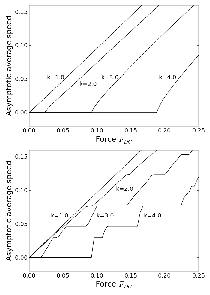
Figure 1: The $v/F_{DC}$ dependency for a DC- (above) and AC- (below) driven standard FK chain, for mean spacing $\rho=245/397$ and different values of $F_{DC},k$. In the AC case, $F_{AC}=0.2$, $\nu_{0}=0.2$

Numerical simulationsFloria96 ; Mazo95 showed that synchronization often asymptotically appears when forcing $f(t)$ is switched on (numerically an infinite chain is approximated with a long finite one with periodic boundary conditions). In the DC case, it was seen that for any initial condition the dynamics is attracted to a synchronized solution, called uniformly sliding solution, as long as the asymptotic average sliding speed is not zero. The asymptotic average sliding speed $v(\rho)$ depends (continuously) only on the forcing $f$ and the mean spacing $\rho$. Numerics further showed that the critical depinning force is not zero if and only if the set of ground states with the mean spacing $\rho$ does not project in any particle coordinate to the entire real line.

As an example, we consider the driven standard FK model given by the equations

$$\frac{du_{j}(t)}{dt} = u_{j+1}-2u_{j}+u_{j-1}+\frac{k}{2\pi}\sin(2\pi u_{j})+f(t)$$

$$f(t) = F_{DC}+F_{AC}\sin(2\pi\nu_{0}t),$$

with parameters $k,F_{DC},F_{AC},\nu_{0}$.

A typical dependence of $v(\rho)$ on $F_{DC}$ in the DC case ($F_{AC}=0$), and in the AC case for a fixed $F_{AC},\nu_{0}$ is in Figure 1.

In the AC case, $v(\rho)$ also depends continuously on $\lambda$ and $\rho$, but is not smooth up to a certain critical value of $F_{DC}$ - the dynamical Aubry transition. Also it was seen that as long as the asymptotic speed is not zero, the solution typically asymptotically synchronizes.

III Mathematical background

III.1 Asymptotics of a solution

In this paper we consider configurations of bounded width, by which we mean configurations $u$ for which there exists mean spacing $\rho(u)$ and a real number such that for some constant $K>0$ and all integers $m,n$,

$$|u_{m}-u_{n}-(m-n)\rho(u)|\leq K.$$ (3)

(With some technical care as done in Ref. Slijepcevic14, but beyond the scope of this paper, all the results also hold on more general space of configurations of bounded spacing, that is satisfying $\sup_{m\in\mathbb{Z}}|u_{m+1}-u_{m}|<\infty$). Denote by $\widetilde{\mathcal{X}}$ the space of all the configurations of bounded width, and with $\widetilde{\mathcal{X}}_{\rho}$ its subspace of configurations with the mean spacing $\rho$. For example, as by the standard result of Aubry-Mather theory all the ground states satisfy (3) with $K=1$ (Ref Bangert88, , Corollary 3.16), they are in $\widetilde{\mathcal{X}}$. By the same argument, the synchronized configurations also satisfy (3) with $K=1$ and are in $\widetilde{\mathcal{X}}$.

Standard results of existence of ODE on Banach spaces imply that (1) generates a smooth semiflow on $\widetilde{\mathcal{X}}$, with $\widetilde{\mathcal{X}}_{\rho}$ being invariant setsBaesens98 ; Baesens05 ; Slijepcevic14 . When considering asymptotics, we consider pointwise convergence of configurations (i.e. the product topology on $\widetilde{\mathcal{X}}$), rather than uniform convergence.

The usual notions of dynamical systems theory make sense only for relatively compact trajectories. Fortunately this holds for initial conditions in $\widetilde{\mathcal{X}}_{\rho}$ if we identify $u$ and $u+n$ for all integer $n$. We denote $\mathcal{X}$, $\mathcal{X}_{\rho}$ to be the quotient sets with respect to that relation, and omit the subscript $n$ in $S_{m,n}$. Now each $\mathcal{X}_{\rho}$ is compact and invariant for both spatial translations $S_{m}$ and the time evolution $T_{t}$, $t\geq 0$ (invariance follows from the order preserving property, Ref. Slijepcevic14, , Section 4).

The usual notion of $\omega$-limit set considers all the limit points of a trajectory as time goes to infinity. Here we consider a typically smaller set of physically the most relevant asymptotic trajectories, which are asymptotically observed with non-zero probability with respect to time and spatial windows. A precise definition follows:

Definition 3

The weak $\omega$-limit set of $u$, denoted by $\widetilde{\omega}(u)$, is the smallest closed set such that for any (arbitrarily small) open neighborhood $U$ of $\widetilde{\omega}(u)$, the ratio of $m,n$, $0\leq m\leq N$, $-N\leq n\leq N$ for which $T_{m}S_{n}u\in U$, converges to $1$ as $N\rightarrow\infty$.

An equivalent definition of $\widetilde{\omega}(u)$ is given in Lemma 14 in the Appendix. It is easy to show that $\widetilde{\omega}(u)$ is a well-defined, closed set and a subset of $\omega(u)$Slijepcevic14 . Unlikely the $\omega$-limit set, $\widetilde{\omega}$ is not necessarily connected. An interpretation of $\widetilde{\omega}$ is that, if we choose randomly a (sufficiently large) time, and a random, arbitrarily large, spatial window of an infinite chain, we will with asymptotic probability $1$ observe a configuration in $\widetilde{\omega}(u)$. We propose the definition of a (space-time) attractor for a spatially extended (i.e. on an infinite domain) system like (2) to be the set $\mathcal{A}$ which is the closure of the union of all weak $\omega$-limit sets,

$$\mathcal{A}=\text{Cl}\left(\bigcup_{u\in\mathcal{X}}\widetilde{\omega}(u)\right).$$

Our definition of $\mathcal{A}$ results with a typically smaller set than attractor as standardly definedMiranville08 . We think our definition is physically relevant. One can say that the standard attractor incorporates all the asymptotics of the dynamics, while our set $\mathcal{A}$ captures asymptotics with non-zero space-time positive probability. Furthermore, if for example a system like (2) is space-time chaotic in the sense of Bunimovich and SinaiBunimovich88 , one can show that the space-time chaos is then contained in $\mathcal{A}$Slijepcevic14a .

III.2 Invariant measures and dynamical phase transitions

In addition to considering evolution of individual configurations with respect to (1), we find useful considering simultaneous evolution of a family of initial configurations and finding average properties of this evolution. We make it precise by considering evolution of probability measures, and more specifically probability measures invariant for the spatial shift.

We can write $S=S_{1}$, $T=T_{1}$ (the time-one map for (2)). Note that there exists a huge number of $S$-invariant probability measures on the state space $\mathcal{X}$. For example, we can embed in $\mathcal{X}$ in many ways the standard Bernoulli probability measure on the space of bi-infinite sequences of $\{0,1\}$. More generally, a $S$-invariant probability measure is any (shift-invariant) random process which constructs a configuration in $\mathcal{X}$.

Given any $S$-invariant measure $\mu$, we can consider its evolution $\mu(t)$ with respect to (1) by considering evolution of each configuration (mathematically, $\mu(t)$ is the pulled measure $\mu(t)=T_{t}^{\ast}\mu(0)$). A $T$-invariant measure is a measure which is also invariant with respect to the evolution (2). The importance of $S,T$-invariant measures on $\mathcal{X}$ is in the following fact:

Proposition 4

The attractor $\mathcal{A}$ coincides with the union of supports of all $S,T$-invariant measures on $\mathcal{X}$. Furthermore, for any $\rho\in\mathbb{R}$, $\mathcal{A}_{\rho}=\mathcal{A\cap X}_{\rho}$ is not empty.

(We postpone the proof of this as most the other other claims to the Appendix.) Thus the study of the attractor $\mathcal{A}$ is equivalent to understanding the structure of $S,T$-invariant measures.

We can now extend the Definition 1 of synchronized configurations and solutions to measures. We say that a synchronized measure is a $S,T$-invariant probability measure such that no two configurations in its support intersect. Clearly by definition, a synchronized measure is supported on synchronized trajectories. Denote by $\mathcal{S}_{\rho}\subset\mathcal{A}_{\rho}$ the union of supports of all the synchronized measures on $\mathcal{X}_{\rho}$. We will see in the next section that $\mathcal{S}_{\rho}$ is not empty.

One typically distinguishes two dynamical phases of (2), depending on whether transport is possible. In the depinned phase, asymptotically each particle can slide over the entire $\mathbb{R}$, while in the pinned phase some of the regions are off-limit as the force is too weak as compared to the potential $V$ and the related Peierls-Nabarro barrierFloria96 . We propose a rigorous way to define pinned vs. depinned phase, which works both in the DC and AC case, by using the language of measures, in the spirit of MatherMather89 .

Let $\pi_{0}:{\cal X}\rightarrow\mathbb{S}^{1}$ be the projection of a configuration $u$ to $u_{0}$ (it projects onto the circle $\mathbb{S}^{1}=\mathbb{R}/\mathbb{Z}$, as we identify $u$ and $u+n$ for integer $n$).

Definition 5

We say that (2) is in the depinned phase for a given mean spacing $\rho\in\mathbb{R}$, if there exists a synchronized measure $\mu$ with the mean spacing $\rho$ such that $\pi_{0}(\textnormal{supp}({\mu}))$ is onto (i.e. the entire $\mathbb{S}^{1}$); otherwise it is in the pinned phase.

Here $\textnormal{supp}(\mu)$ denotes the support of $\mu$. Note that, as we consider $S$-invariant measures, this definition is independent of the projected coordinate. For a given one-parameter family of FK-chains or forces $f(t)$, the dynamical Aubry transition for a given $\rho\in\mathbb{R}$ is the value of the parameter in which the pinned/depinned phase changes.

Equivalence of the definition of depinned/pinned phases as above to analyticity (resp. non-analyticity) of modulation functions, as well as to the dependence of the average speed on average driving force as described in subsection II.3, was essentially shown by QinQin11 ; Qin13 .

Analogously to thermodynamics, one can expect that the difference in phases of (2) is whether there is a unique (ergodic) $S,T$-invariant measure with a chosen mean spacing or not. We will see later that this is indeed a characterization if $\rho$ is irrational (also for rational $\rho$ with additional technical restrictions): the $S,T$-invariant measure is unique in and strictly in the depinned phase.

III.3 Dynamics of intersections of solutions

The key feature of the dynamics (2), that it is order-preserving, was used by Middleton, Baesens and MacKayBaesens98 ; Baesens05 ; Middleton92 , in proving results on asymptotics of (mostly) finite chains with DC dynamics. We will here use a generalization of that related to counting intersections of two solutions. We already introduced the notion of intersection of two configurations. It is important to distinguish transversal and non-transversal intersections, as in Figure 2 (see Ref. Slijepcevic14, for a precise classification).

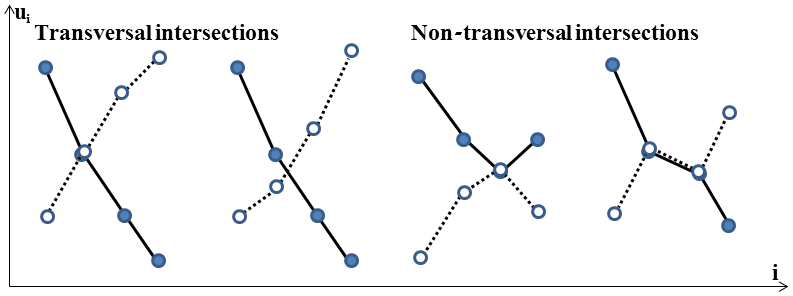
Figure 2: Examples of transversal and non-transversal intersections of configurations.

A stronger version of the order-preserving rule is that, if $u(0)$ and $v(0)$ are two chain configurations with at most finite number of intersections, then the following is known and can be proved by considering linearization of (2) (Ref. Slijepcevic14, , Sections 3 and 4):

(I1)

The number of intersections of $u(t)$ and $v(t)$ is a non-increasing function of $t$,

(I2)

If $u(t)$ and $v(t)$ intersect non-transversally at $t_{0}$, then the number of intersections strictly drops at $t=t_{0}$.

These ideas originate from 1D parabolic PDE’s, where they have been extensively used to describe their asymptoticsAngenent88a ; Fiedler89 ; Joly10 . They are, however, not directly applicable to the dynamics (2) (or also to PDE’s on unbounded domains), as two arbitrary configurations $u,v$ (with the same mean spacing) typically intersect infinitely many times. We resolve this by considering an average number of intersections with respect to a probability measure on the state space $\mathcal{X}$. Precisely, let $\mathcal{I}(u,v)\in\{0,1\}$ be the function which assigns $1$ if $u,v$ intersect in the interval $[0,1)$, otherwise it is $0$. If $\mu\,\$is any $S$-invariant probability measure on $\mathcal{X}$, we define the average number of self-intersections of $\mu$ as

$$\mathcal{I}(\mu)=\sum_{n\in\mathbb{Z}}\int\mathcal{I}(u+n,v)d\mu(u)d\mu(v)\text{.}$$ (4)

The meaning of (4) is the following: the expression $\int I(u,v)d\mu(u)d\mu(v)$ is the probability that two randomly chosen configurations $u,v$ intersect in the interval $[0,1)$. As $\mathcal{\mu}$ is invariant for the spatial shift $S$, this is also the probability of finding an intersection in any interval $[m,m+1)$. We have a sum over $n$ in the definition of $\mathcal{I(\mu)}$ to make sure it is well defined on the quotient space $\mathcal{X}$, as we identify configurations $u$ and $u+n$. It is easy to check $\mathcal{I(\mu)}$ is always finiteSlijepcevic14 . One can now show that $\mathcal{I(\mu)}$ has properties mimicking (I1), (I2), without any restrictions to chosen configurations and measures. A rigorous proof of the following is in Ref. Slijepcevic14, ; we sketch the argument in the Appendix.

Theorem 6

If $\mu$ is an $S$-invariant probability measure with evolution $\mu(t)$ with respect to (2), then:

(M1)

The function $t\mapsto\mathcal{I(}\mu(t)\mathcal{)}$ is non-increasing;

(M2)

If for some $t_{0}$, there are $u$, $v$ in the support of $\mu(t_{0})$ with a non-transversal intersection, then $t\mapsto\mathcal{I(}\mu(t)\mathcal{)}$ is strictly decreasing at $t_{0}$ (i.e. $\mathcal{I(}\mu(t+\varepsilon)\mathcal{)<I(}\mu(t-\varepsilon)\mathcal{)}$ for any $\varepsilon>0$).

The property (M1) means that $\mathcal{I}$ is a Lyapunov function on the space of $S$-invariant measures. As for synchronized measures, $\mathcal{I}$ reaches its minimum zero (see the comment after Theorem 7 below), these measures are expected to be Lyapunov stable. We deduce implications of this to asymptotics of individual trajectories in Section V.

IV 2D representation of the attractor

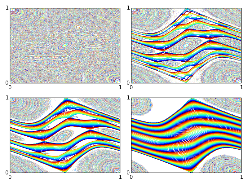
Figure 3: 2D representations of the attractor of a DC-driven standard FK chain with $k=1.0$. The DC force (left to right): $F=0$, $0.001$, $0.005$, $0.05$. The same color corresponds to the same configuration (i.e. the same orbit with respect to $h$ acting on $\mathbb{S}_{1}\times\mathbb{R}$) and its time evolution.

We now show that the attractor $\mathcal{A}$ of the dynamics (2) can be represented as a $2$-dimensional map, which will be important for both qualitative and quantitative description of the dynamics. This fact has been extensively studies in the case $f=0$, as noted in Section II. It is somewhat unexpected that this principle extends for arbitrary DC and AC forcing. We define the projection $\pi:\mathcal{A}\rightarrow\mathbb{S}^{1}\times\mathbb{R}$ with

$$\pi(u)=(u_{0},u_{1}-u_{0})\text{.}$$

Theorem 7

Any two configurations $u,v\in\mathcal{A}$ can not intersect non-transversally. Furthermore, $\pi$ is injective.

This follows directly from Theorem 6 (details in the Appendix). A direct consequence is that synchronized measures are characterized as $S,T$-invariant measures $\mu$ for which $\mathcal{I}(\mu)=0$. Here is why: if $\mathcal{I}(\mu)=0$, then by continuity the only possible intersections in the support of $\mu$ are non-transversal, which is impossible.

Projection $\pi$ enables us now to visualize and analyze $\mathcal{A}$ in 2D, as done in Figure 3, plotting images of the projected spatial shift map $h=\pi\circ S\circ\pi^{-1}$ in the same color. As we identified orbits $u$ and $u+n$ for integer $n$, the map $h$ is well defined on the cylinder $\mathbb{S}_{1}\times\mathbb{R}$, and can be understood as a dynamical analogue of an area-preserving twist map on the cylinder which describes the attractor in the case with no force.

We will see that the approximately level circles (”rainbows” in Figure 3) correspond to depinned synchronized trajectories, with the average coordinate $p$ corresponding to the mean spacing $\rho$. We call them KAM-circles (borrowing terminology from the Hamiltonian dynamics), and define them as homotopically non-trivial (i.e. not compressible to a fixed point) invariant circles of the function $h$ on $\mathbb{S}_{1}\times\mathbb{R}$. Analysis of the pinned/depinned phase transition will rely on the 2D representation as in Figure 3, and will use the following:

Theorem 8

Given any mean spacing $\rho\in\mathbb{R}$, the set $\mathcal{S}_{\rho}$ is not empty. In the depinned phase, $\mathcal{A}_{\rho}=\mathcal{S}_{\rho}$ and it projects to a KAM-circle.

The converse of the last statement in Theorem 8 also holds. Given a map $h$ and a point $x=\pi(u)\in\mathbb{S}_{1}\times\mathbb{R}$, one can recover the mean spacing of $u$ by calculating the rotation number of $x$ with respect to $h$, defined as the average of the first coordinate of $h$-iterates of $x$. By adapting the proof of Theorem 8 given in the Appendix, one can also show that if (2) is the pinned phase for a given $\rho$, then $h$ does not have a KAM-circle with that rotation number. We omit the proof.

An implication is that the structure of synchronized orbits, when projected to the cylinder, is analogous to the structure of ground states when projected to the cylinder. Thus we can use tools from Hamiltonian dynamics as outlined in the next section.

We now come back to the definition of the pinned vs. depinned phase and its characterization.

Corollary 9

If $\rho$ is irrational and (2) in the depinned phase, then there is a unique ergodic $S,T$-invariant measure with the mean spacing $\rho$.

The converse of Corollary 9 also holds, and can be shown by adapting the construction of Mather’s connecting orbits of area-preserving twist mapsMather93 ; Slijepcevic99 and related invariant measures. This would result with a rich family of ergodic $S,T$-invariant measures with the same (pinned) rotation number; we omit details of the construction.

Finally, the following fact regarding intersection of depinned synchronized configurations will be the key in applications.

Corollary 10

If (2) is in the depinned phase for $\rho\in\mathbb{R}$, given any $u\in\mathcal{A}_{\rho}$, no configuration in $\mathcal{A}$ can intersect $u$ more than once.

V Synchronized orbits are attracting

Attractiveness and global stability (in the sense of definitions in Section III, i.e. ignoring probability/density 0 times and space windows) of synchronized orbits in the depinned phase is now straightforward.

Corollary 11

Assume (2) is in the depinned phase for a given $\rho\in\mathbb{R}$. Then for any $u\in\mathcal{X}_{\rho}$, $\widetilde{\omega}(u)$ consists of (depinned) synchronized orbits, i.e. $\widetilde{\omega}(u)\subset\mathcal{S}_{\rho}$.

Proof. By definition, $\widetilde{\omega}(u)\subset\mathcal{A}_{\rho}$, and by Theorem 8, $\mathcal{A}_{\rho}=\mathcal{S}_{\rho}$.   

In the pinned phase, one can not expect such general results. For example, even in the stationary case $f(t)=0$, the structure of the pinned part of $\mathcal{A}$ is quite complex (it is analogous to understanding Birkhoff regions of instability of area-preserving twist maps, whose complexity is still not fully understood). We can, however, describe a relatively rich family of configurations in the basin of attraction of $\mathcal{S}_{\rho}$: ground states of FK model with defects (discommensurations), that is with missing or squeezed in extra particles within the ground state structureBraun:04 ; Floria96 . The following abstract definition generalizes this notion: we say that a configuration $u$ has $k$ defects, if $k$ is the maximal number of intersections of $u$ and $S_{m,n}u$ over all integers $m,n$.

Theorem 12

In the DC case, if $u\in\mathcal{X}_{\rho}$ has finitely many defects, then $\widetilde{\omega}(u)\subset\mathcal{S}_{\rho}$.

The proof of that in the Appendix could be also extended to hold in the AC case and for configurations with zero defect density. We intend to provide details on that separately.

VI Conclusion

VI.1 Numerical determination of dynamical phase transitions

As an example of an application of tools from Hamiltonian dynamics enabled by our 2d representation of the attractor, we consider tools known as Converse KAM. These algorithms focus on break-up of KAM-circles and more generally KAM tori. They have beem developed in the context of area-preserving twist maps: by MacKay and StarkMacKay85 (based on earlier works of Mather, Herman and others); Boyland and HallBoyland87 , and GreeneGreene79 . The first two are based on a simple characterization: KAM-circles are ”barriers for transport”, which, expressed in terms of intersections of configurations, states that no configuration (associated to an orbit) can intersect a KAM-configuration more than once. As this is by Corollary 10 indeed a property of depinned synchronized configurations, the Converse KAM algorithms should be applicable.

For example, the Boyland-Hall algorithm can be applied to determining the dynamical phase transition in the DC phase as follows. Assume $u$ is a stationary periodic configuration of (1) of the type $(p,q)$; that means $T_{t}(u)=u$ for all $t$, and $u_{k+q}=u_{k}+p$ for all $k$. We define its rotation band $r(u)=(r^{-}(u),r^{+}(u))$, where

$$r^{-}(u) = \min_{j,k=1,...,q}\frac{\left\lceil u_{j+k}-u_{j}\right\rceil}{k},$$

$$r^{+}(u) = \max_{j,k=1,...,q}\frac{\left\lfloor u_{j+k}-u_{j}\right\rfloor}{k}.$$

Here $\left\lceil x\right\rceil$ is the smallest integer larger than $x$, and $\left\lfloor x\right\rfloor$ the largest integer smaller than $x$. Let ${\cal R}$ be the union of all the rotation bands for all the stationary periodic configurations.

The algorithm is based on the following Theorem

Theorem 13

The system (2) with DC driving is in the pinned phase for a given mean spacing $\rho\in\mathbb{R}$, if and only if $\rho\in{\cal R}$.

The proof is an application of Corollary 10 and techniques from Ref. Boyland87, and will be reported in Ref. Nincevic14, . As we can numerically find stationary periodic configurations (by finding extremal points of a ”tilted” energy functional $H$ restricted to the periodic configurations) and calculate their rotation bands, the phase diagram can be calculated with arbitrary precision.

VI.2 Perspectives

One can question whether the results on infinite chains are only of theoretical interest, as all systems in nature are finite. We argue that analyzing such extended dynamical systems is the right tool to obtain bounds (for example on relaxation times) independent of the system size. For example in Ref. Gallay14, we used that approach to find bounds on relaxation times of the viscous fluid turbulence independent of the reservoir size, and in Refs. Gallay:01, , Gallay:12, , to many other systems. Our results imply that for FK models, there exist bounds on convergence times to synchronized solutions independent of the chain size. It is an important next step to find them.

The description of the dynamics of driven FK models here is not complete, as we described only the ”non-zero space-time probability” asymptotics. A complete asymptotics description is most likely a combination of the 2D, typically synchronized, dynamics we described, and coarsening as described by Eckmann and RougemontEckmann98 for a similar system. That means that different parts of the chain converge to different dynamical ground states, and then they either diffusively or in a sequence of discrete coarsening ”jumps” coallesce on larger and larger space and time scales. A more precise description of this dynamics would be nice.

The results here apply also to more general 1D chains whose energy is given by a function $V(u_{j},u_{j+1})$ satisfying the twist condition $\partial_{xy}V(x,y)\leq-\delta<0$, as long as the interaction is only between the nearest neighbours. For longer range interactions, even if the dynamics is cooperative (i.e. the off-diagonal elements of the linearized equation are positive), the intersection-counting tools do not applySlijepcevic14 . The approach is, however, applicable to the ratchet dynamics of FK chains (no driving; but either the site potential or the interaction potential change periodically in time), where exact results are scarceFloria05 . Furthermore, it applies also to the second order dynamics as long as damping is strong enough, and to analogous continuous space systemsSlijepcevic14a .

Finally, we propose focusing on the attractor as defined here, or equivalently on description of the space-time invariant measures, when studying any extended dynamical system (by that we mean lattice systems of infinitely many ODESlijepcevic13 ; or PDE on unbounded domainsGallay:01 ; Gallay:12 ). This should result with, for example, better understanding of existence and frequency of occurrence of the space-time chaos, as our understanding of that phenomenon is quite limitedBunimovich88 ; Mielke09 .

*

Appendix A Proofs of Theorems

In all the proofs we use the fact that $\mathcal{X}_{\rho}=\widetilde{\mathcal{X}}_{\rho}/\sim$ is compact in the (always implicitly assumed) induced product topology, which follows from the Tychonoff theorem. Here $\widetilde{\mathcal{X}}$, $\widetilde{\mathcal{X}}_{\rho}$ are the sets of configurations of bounded width as defined in Section III.A, $\sim$ is the relation of equivalence, $u\sim u+n$ for any integer $n$. As in most of the paper, we abuse the notation and denote by $u$ both configurations in $\mathcal{X}$ and their representatives in $\widetilde{\mathcal{X}}$. All the measures are Borel probability measures on $\mathcal{X}_{\rho}$ or $\mathcal{X}$. By the Alaoglu theorem, the set of probability measures on $\mathcal{X}_{\rho}$ is compact in the weak* topology. We always assume without loss of generality that an ($T$- or $S$-invariant) measure on $\mathcal{X}$ is actually supported on $\mathcal{X}_{\rho}$ for some $\rho\in\mathbb{R}$. We can do that by the Ergodic Decomposition TheoremKatok95 , as $\mathcal{X}_{\rho}$ is $S$- and $T$-invariant. All the proofs are done by considering the invariance with respect to the time-one map $T=T_{1}$. They could be easily adjusted to the DC case with invariance being considered with respect to the semiflow $T_{t}$, $t\geq 0$.

Prior to the proof of Proposition 4, we introduce characterization of $\widetilde{\omega}$-limit sets. Denote by $\mathbf{1}_{\mathcal{V}}$ the characteristic function of a set $\mathcal{V}$.

Lemma 14

A configuration $v\in\widetilde{\omega}(u)$ if only if for each open neighbourhood $\mathcal{V}$ of $v$, there exists $\delta>0$ and a sequence $N_{k}\rightarrow\infty$ such that

$$\frac{1}{(N_{k}+1)(2N_{k}+1)}\sum_{n=0}^{N_{k}}\sum_{m=-N_{k}}^{N_{k}}\mathbf{1}_{\mathcal{V}}({T_{n}S_{m}v})\geq\delta.$$

Proof. Straightforward, by contradiction.   

Proof of Proposition 4. We first show that each $v\in\widetilde{\omega}(u)$ is in the support of some $S,T$-invariant measure. Choose an open neighborhood $\mathcal{V}$ of $v\in\widetilde{\omega}(u)$, and find $\delta>0$ and a sequence $N_{k}\rightarrow\infty$ as in Lemma 14. Let $\mu_{k}$ be a sequence of measures on $\mathcal{X}_{\rho}$ defined as

$$\mu_{k}=\frac{1}{(N_{k}+1)(2N_{k}+1)}\sum_{n=0}^{N_{k}}\sum_{m=-N_{k}}^{N_{k}}\delta_{T_{n}S_{m}u},$$

where $\delta_{u}$ is the Dirac measure supported on $u$. It is easy to check that the limit $\nu$ of each convergent subsequence of $\mu_{k}$ (which exists due to compactness) is a $S,T$-invariant measure on $\mathcal{X}_{\rho}$.

Now choose a sequence of decreasing open neighborhoods $\mathcal{V}_{n}$ of a fixed $v\in\widetilde{\omega}(u)$ such that $\cap_{n\in\mathbb{N}}\mathcal{V}_{n}=\{v\}$ and construct a sequence of associated $S,T$-invariant measures $\nu_{n}$ as above. Then $v$ is in the support of the $S,T$-invariant measure $\sum_{n\in\mathbb{N}}(1/2^{n})\nu_{n}$.

The converse follows from the fact that the union of supports of all the $S,T$-invariant measures is closed (Ref. Slijepcevic14a, , Lemma 2.1) and a standard ergodic-theoretical argument based on the Birkhoff Ergodic Theorem and the Ergodic Decomposition Theorem. As logically not required for the results that follow, we omit the details.

The set $\mathcal{A}_{\rho}$ is not empty, as $\mathcal{X}_{\rho}$ is compact, $S,T$-invariant, thus it supports a $S,T$-invariant measure (Ref. Slijepcevic14, , Lemma 7.2).   

Outline of proof of Theorem 6. A detailed proof is given in Ref. Slijepcevic14, , Propositions 5 and 6; we outline the key argument. Consider the function

$$\mathcal{I}(\mu(t))=\sum_{n\in\mathbb{Z}}\int\mathcal{I}(u(t),v(t)+n)d\mu(u(0))d\mu(v(0)),$$

counting intersections of $u,v$ with respect to the time evolution of a measure $\mu$. An intersection of $u(t)$, $v(t)$ can be represented by a continuous curve $\gamma(t)$, which is defined as the point where the graph of $i\mapsto u_{i}(t)-v_{i}(t)$ crosses the $x$-axis. As by property (I1), the function $\mathcal{I}(u(t),v(t)+n)$ is non-increasing (except in the cases when $\gamma(t)$ crosses the boundaries of $[0,1]$ which can be shown to by $S$-invariance of $\mu$ cancel out), $\mathcal{I}(\mu(t))$ is non-increasing. Similarly, a continuity argument and (I2) imply (M2).   

Proof of Theorem 7. By Proposition 4, we can assume $u$, $v$ are in the support of some $S,T$-invariant measure $\mu$ (if not the same measure, we take their convex combination $\mu=\mu_{1}/2+\mu_{2}/2$ and obtain again a $S,T$-invariant measure). If $u$, $v$ intersect non-transversally, by Theorem 6, $\mathcal{I}(\mu(t))$ is strictly decreasing at $t=0$. But $\mu$ is $T$-invariant, thus $\mathcal{I}(\mu(t))$ must be constant, which is a contradiction. Now, if $\pi(u)=\pi(v)$ for some $u,v\in\mathcal{A}$, by definition they intersect non-transversaly, which is impossible.   

Prior to the proof of Theorem 8, we need an intermediate result. Assume (2) is in the depinned phase for some $\rho\in\mathbb{R}$. Denote by $\mathcal{S}^{*}_{\rho}$ the support of the synchronized measure $\mu$ from Definition 5.

Lemma 15

If $u\in\mathcal{S}^{*}_{\rho}$, depinned, then no configuration in $\mathcal{A}$ can intersect $u$ more than once.

Proof. By definition, $\pi_{0}:\mathcal{S}^{*}_{\rho}\rightarrow\mathbb{S}^{1}$ is bijective (injective due to synchronization; onto as in the depinned phase). Thus its lift $\widetilde{\mathcal{S}}^{*}_{\rho}$ (i.e. not considered as a quotient space) is an image of a continuous curve $\gamma:\mathbb{R}\rightarrow\widetilde{\mathcal{A}}$, $\gamma(0)=u$, increasing in each coordinate. Assume some $v\in\widetilde{\mathcal{A}}$ intersects $u$ twice, say between $j,j+1$ and $k,k+1$. Without loss of generality let $v_{j}\leq u_{j}$, $v_{j+1}>u_{j+1},...,v_{k-1}>u_{k-1},v_{k}\geq u_{k}$, $v_{k+1}<u_{k+1}$. Let $s>0$ be the largest $s$ such that $\gamma(s)$ and $v$ intersect between $j,...,k+1$. By continuity of $\gamma$, $\gamma(s)$ and $v$ intersect non-transversally, which is in contradiction to Theorem 7.   

Proof of Theorem 8. Let $\rho\in\mathbb{R}$. We first show that $\mathcal{S}_{\rho}$ is not empty. Choose a synchronized orbit $u$ in $\mathcal{X}_{\rho}$ (which exists by Theorem 2). Let $\mathcal{B}$ be the smallest, closed, $S,T$-invariant set containing $u$. As (3) holds with $K=1$, we see that $\mathcal{B}\subset\mathcal{X}_{\rho}$. Thus $\mathcal{B}$ is compact. By definition and continuity, if two configurations in $\mathcal{B}$ intersect, they must intersect non-transversally. Compactness of $\mathcal{B}$ implies that there exists a $S,T$-invariant measure $\mu$ supported on $\mathcal{B}$. As $\mathcal{B}$ contains no transversal intersections, $\mu$ by Theorem 7 contains no intersections at all. It is then by definition synchronized, thus $\mathcal{S}_{\rho}$ is not empty.

To show that $\mathcal{A}_{\rho}=\mathcal{S}_{\rho}$, it suffices to show that $\mathcal{A}_{\rho}=\mathcal{S}^{*}_{\rho}$. Here $\mathcal{S}^{*}_{\rho}=\textnormal{supp}(\mu)$, $\mu$ are as defined prior to Lemma 15. Choose any $v\in\mathcal{A}_{\rho}$. By Proposition 4, $v$ is in the support of a $S,T$-invariant measure $\zeta$. By definition of $\mu$, we can find $u$ in the support of $\mu$ such that $u_{0}=v_{0}$. If $u\not=v$, by Lemma 10 $u,v$ intersect exactly once. Now $\mu\times\zeta$ is a probability measure on $\mathcal{A}_{\rho}\times\mathcal{A}$, invariant for $S\times S$. If $U,V$ are small enough neighborhoods of $u,v$ in $\mathcal{A}_{\rho}$ such that any two configurations in $U,V$ also intersect at site $0$, by Poincaré recurrence applied to $S\times S$ on $U\times V$, we can find $u^{\prime}\in U$, $v^{\prime}\in V$ such that $u^{\prime},v^{\prime}$ intersect infinitely many times. As by (3), there exists $K$ such that for all $j\in\mathbb{Z}$, $|u_{j}-v_{j}|\leq K$ (as they have the same mean spacing), we can find their representatives in $\widetilde{\mathcal{A}}_{\rho}$ which intersect infinitely many times, which is in contradiction to Lemma 15.

Now as $\mathcal{A}_{\rho}=\mathcal{S}_{\rho}=\mathcal{S}^{*}_{\rho}$, by definition of the depinned phase and $\mathcal{S}^{*}_{\rho}$ it must project to a KAM-circle.   

Proof of Corollary 9. Uniqueness of the $S,T$-invariant measure for irrational $\rho$ follows from the Denjoy theory (in that case there is an unique $S$-invariant measure, Ref. Katok95, , Section 12.7).   

Proof of Corollary 10. In the proof of Theorem 8 above we showed that in the depinned phase, $\mathcal{A}_{\rho}=\mathcal{S}^{*}_{\rho}$. Thus the claim follows from Lemma 15.   

In the proof of Theorem 12 we will require the following, which was proved in Ref. Slijepcevic14, , Theorem 1.4.

Theorem 16

In the DC case, the attractor $\mathcal{A}$ consists of equilibria and depinned synchronized trajectories.

Here equilibria are configurations $u$ for which $\partial u/\partial t=0$.

Proof of Theorem 12. If $u$ has at most $k$ defects, $u$ and any translate $S_{m,n}u$ intersect at most $k$ times. By continuity, as $\widetilde{\omega}(u)\subset\omega(u)$ and as trajectories in $\widetilde{\omega}(u)$ by Theorem 7 can not intersect non-transversally, for any $v\in\widetilde{\omega}(u)$, $v$ and $S_{n,m}v$ intersect at most $k$ times. By Theorem 16, $v$ is either depinned synchronized (so the proof is done), or an equilibrium. If $v$ is an equilibrium, it is in the support of a $S$-invariant measure $\mu$ supported on the closure (in $\mathcal{X}_{\rho}$) of $S_{n}v$, $n\in\mathbb{Z}$, thus supported on equilibria. As the number of self-intersections of two configurations in the support is finite and bounded by $k$, one can (e.g. by the Birkhoff Ergodic Theorem) easily show that $\mathcal{I(\mu)=}0$. Thus all $v$ in the support of $\mathcal{\mu}$ must be synchronized.

References

- (1) S. Angenent and B. Fiedler, The dynamics of rotating waves in scalar reaction diffusion equations, Trans. Am. Math. Soc. 307 (1988), 545-568.
- (2) S. Aubry and P. Y. Le Daeron, The discrete Frenkel-Kontovora model and its extensions, Physica D 8 (1983), 381.422.
- (3) C. Baesens, R. S. Mackay, Gradient dynamics of tilted Frenkel-Kontorova models, Nolinearity 11 (1998), 949-964.
- (4) C. Baesens, Spatially extended systems with monotone dynamics (continuous time). Dynamics of coupled map lattices and of related spatially extended systems, 241-263, Lecture Notes in Phys. 671, Springer (2005).
- (5) V. Bangert, Mather sets for twist geodesics on tori, Dynamics Reported 1 (1988), 1-55.
- (6) P. Boyland and G. Hall, Invariant circles and the order structure of periodic orbits in monotone twist maps, Topology 113 (1987), 21-35.
- (7) O. M. Braun and Y. S. Kivshar, The Frenkel-Kontorova Model. Concepts, methods, applications. Springer-Verlag, Berlin, 2004.
- (8) L. Bunimovich and Y. Sinai, Spacetime chaos in coupled map lattices, Nonlinearity 1 (1988), 491-516.
- (9) J.-P. Eckmann and J. Rougemont, Coarsening by Ginzburg-Landau dynamics, Comm. Math. Phys. 199 (1998), 441-470.
- (10) B. Fiedler, J. Mallet-Paret, A Poincaré-Bendixson theorem for scalar reaction diffusion equations, Arch. Rational Mech. Anal. 107 (1989), 325-345.
- (11) L. M. Floria and J. J. Mazo, Dissipative dynamics of the Frenkel-Kontorova model, Advances in Physics, 45 (1996), 505-598.
- (12) L. M. Floria, C. Baesens and J. Gómez-Gardenez, The Frenkel-Kontorova model, in Dynamics of Coupled Map Lattices and of Related Spatially Extended Systems, Lecture Notes in Phys. 671, Springer, Berlin, 2005, 209-240.
- (13) Th. Gallay and S. Slijepčević, Energy flow in formally gradient partial differential equations on unbounded domains. J. Dynam. Differential Equations 13 (2001), 757-789.
- (14) Th. Gallay and S. Slijepčević, Distribution of Energy and Convergence to Equilibria in Extended Dissipative Systems, to appear in J. Dynam. Differential Equations.
- (15) Th. Gallay and S. Slijepčević, Uniform boundedness and long-time asymptotics for the two-dimensional Navier-Stokes equations in an infinite cylinder, to appear in J. Math. Fluid Mech.
- (16) J. M. Greene, A method for determining a stochastic transition, J. Math. Phys. 20 (1979), 1183.
- (17) B. Hu, W. Qin and Z. Zheng, Rotation number of the overdamped Frenkel-Kontorova model with ac-driving, Physica D, 208 (2005), 172-190.
- (18) R. Joly, G. Raugel, Generic Morse-Smale property for the parabolic equation on the circle, Ann. Inst. H. Poincaré 27 (2010), 1397-1440.
- (19) A. Katok and B. Hasselblatt, Introduction to the Modern Theory of Dynamical Systems. Cambridge University Press, 1995.
- (20) R. S. MacKay and I. Percival, Converse KAM: theory and practice, Commun. Math. Phys. 98 (1985), 469-512.
- (21) J. Mather, Existence of quasi-periodic orbits for twist homeomorphisms of the annulus, Topology 21 (1982), 457-467.
- (22) J. Mather, Minimal measures, Comm. Math. Helvetici 64 (1989), 375-394.
- (23) J. Mather, Variational construction of connecting orbits, Ann. Inst. Fourier, Grenoble 43 (1993), 1349-1386.
- (24) J. J. Mazo, F. Falo and L. M. Floria, Stability of metastable structures in dissipative ac dynamics of Frenkel-Kontorova models, Phys. Rev. B, 52 (1995), 6451-6457.
- (25) A. A. Middleton, Asymptotic uniqueness of the sliding state for charge density waves, Phys. Rev. Lett. 68 (1992), 670-673.
- (26) A. Mielke and S. Zelik, Multi-pulse evolution and space-time chaos in dissipative systems, Mem. Amer. Math. Soc. 198 (2009), 97pp.
- (27) A. Miranville, S. Zelik, Attractors for dissipative partial differential equations in bounded and unbounded domains, Handbook of differential equations: evolutionary equations. Vol. IV, 103-200, Elsevier/North-Holland, Amsterdam, 2008.
- (28) M. Ninčević, B. Rabar and S. Slijepčević, Converse KAM theory and dynamical phase transitions of Frenkel-Kontorova models, in preparation.
- (29) Wen-Xin Qin, Dynamics of the Frenkel-Kontorova model with irrational rotation number, Nolinearity 23 (2010), 1873-1886.
- (30) Wen-Xin Qin, Existence and modulation of uniform sliding states in driven and overdamped particle chains, Comm. Math. Physics 311 (2011), 513-538.
- (31) Wen-Xin Qin, Existence of dynamical hull functions with two variables for the ac-driven Frenkel-Kontorova model, J. Diff. Equations 255 (2013), 3472-3490.
- (32) S. Slijepčević, Monotone gradient dynamics and Mather’s shadowing, Nonlinearity 12 (1999), 969-986.
- (33) S. Slijepčević, The energy flow of discrete extended gradient systems, Nonlinearity 26 (2013), 2051-2079.
- (34) S. Slijepčević, The Aubry-Mather theorem for driven generalized elastic chains, Disc. Cont. Dyn. Systems A 34 (2014), 2983-3011.
- (35) S. Slijepčević, Entropy of scalar reaction-diffusion equations, to appear in Math. Bohemica.