Low-Pass Filters, Fourier Series and
Partial Differential Equations

Abstract

When Fourier series are used for applications in physics, involving partial differential equations, sometimes the process of resolution results in divergent series for some quantities. In this paper we argue that the use of linear low-pass filters is a valid way to regularize such divergent series. In particular, we show that these divergences are always the result of oversimplification in the proposition of the problems, and do not have any fundamental physical significance. We define the first-order linear low-pass filter in precise mathematical terms, establish some of its properties, and then use it to construct higher-order filters. We also show that the first-order linear low-pass filter, understood as a linear integral operator in the space of real functions, commutes with the second-derivative operator. This can greatly simplify the use of these filters in physics applications, and we give a few simple examples to illustrate this fact.

1 Introduction

One of the many important uses of Fourier series is in the role of tools for the solution of boundary value problems involving partial differential equations in Cartesian or cylindrical coordinates [1]. From a historical point of view, one may say that this is, in fact, the original use of these series. In this type of application the final solution of the boundary value problem is obtained in the form of a Fourier series, and the real function that gives its coefficients is not immediately available in closed form. This is not surprising, since the determination of the function is the very essence of the boundary value problem. It is often necessary to take derivatives of the solutions obtained, in order to calculate physical quantities of relevance within the applications, and in some cases the term-wise differentiation of the Fourier series obtained for the solution results in a divergent series.

This is usually brought about by overly simplified initial conditions or boundary conditions, which are used when formulating the physical problem in order to simplify the sequence of operations leading to the solution in the form of a Fourier series. Common cases in which this can happen are the calculation of the acceleration in problems with the vibrating string, the calculation of the electric field in problems involving the electrostatic potential within a box and the calculation of the heat flux density in problems involving the heat equation in solids. Some simple examples on these lines are examined briefly in Appendix B, in order to illustrate the main points of this paper.

In this paper we show that certain low-pass filters can be used to deal with such situations in a way that changes the mathematics so as to make the relevant Fourier series converge, while at the same time changing nothing of importance in the physics involved. The first-order linear low-pass filter is defined in precise mathematical terms, and several of its main properties are established, both on the real line and within a periodic interval. The first-order filter is then used to define higher-order filters, the use of which not only results in convergent Fourier series, but in series that also converge faster and to smoother functions, allowing one to take a few term-by-term derivatives, as needed within the applications involved.

Although the concept of a low-pass filter originates from an engineering practice, it can be defined theoretically in precise mathematical terms, as an operation on real functions. In fact, all the linear low-pass filters discussed here can be understood as integral operators acting in the space of integrable real functions. They can be expressed by integrals on the real line, involving certain kernel functions. They can be defined both on the whole real line and within a periodic interval such as $[-\pi,\pi]$, which allows one to write Fourier expansions for the real functions, in the form

$$f(x)=\frac{1}{2}\,\alpha_{0}+\sum_{k=1}^{\infty}\left[\alpha_{k}\cos(kx)+\beta_{k}\sin(kx)\right],$$

where the coefficients are given by

$$\alpha_{k} = \frac{1}{\pi}\int_{-\pi}^{\pi}dx\,\cos(kx)f(x),$$

$$\beta_{k} = \frac{1}{\pi}\int_{-\pi}^{\pi}dx\,\sin(kx)f(x).$$

Since boundary value problems typically involve partial differential equations within compact domains, it is of particular importance to determine the action of the low-pass filters on functions defined on compact intervals. We will also establish how the filters act directly on the Fourier representations of these functions.

2 The Low-Pass Filters on the Real Line

The low-pass filters are defined as operations on real functions leading to other related real functions. Let us define the simplest such filter, namely the first-order linear low-pass filter. Given a real function $f(x)$ on the real line of the coordinate $x$, of which we require no more than that it be integrable, we define from it a filtered function $f_{\varepsilon}(x)$ by

$$f_{\varepsilon}(x)=\frac{1}{2\varepsilon}\int_{x-\varepsilon}^{x+\varepsilon}dx^{\prime}\,f\!\left(x^{\prime}\right),$$ (1)

where $\varepsilon$ is a strictly positive real constant, usually meant to be small by comparison to some physical scale, and which we will refer to as the range of the filter. One can also define $f_{0}(x)$ by continuity, as the $\varepsilon\to 0$ limit of this expression, which is mostly but not always identical to $f(x)$. The transition from $f(x)$ to $f_{\varepsilon}(x)$ constitutes an operation within the space of real functions. A discrete version of this operation is known in numerical and graphical settings as that of taking running averages. Another similar operation is known in quantum field theory as block renormalization. What we do here is to map the value of $f(x)$ at $x$ to its average value over a symmetric interval around $x$. This results in a new real function $f_{\varepsilon}(x)$ that is smoother than the original one, since the filter clearly damps out the high-frequency components of the Fourier spectrum of $f(x)$, as will be shown explicitly in what follows.

The filter can be understood as a linear integral operator acting in the space of integrable real functions. It may be written as an integral over the whole real line involving a kernel $K_{\varepsilon}\!\left(x-x^{\prime}\right)$ with compact support,

$$f_{\varepsilon}(x)=\int_{-\infty}^{\infty}dx^{\prime}\,K_{\varepsilon}\!\left(x-x^{\prime}\right)f\!\left(x^{\prime}\right),$$

where the kernel is defined as $K_{\varepsilon}\!\left(x-x^{\prime}\right)=1/(2\varepsilon)$ for $|x-x^{\prime}|<\varepsilon$, and as $K_{\varepsilon}\!\left(x-x^{\prime}\right)=0$ for $|x-x^{\prime}|>\varepsilon$. This kernel is a discontinuous even function of $\left(x-x^{\prime}\right)$ that has unit integral. If the functions one is dealing with are defined in a periodic interval such as $[-\pi,\pi]$, then the integral above has to be restricted to that interval, and the kernel can be easily expressed in terms of a convergent Fourier series,

$$K_{\varepsilon}\!\left(x-x^{\prime}\right)=\frac{1}{2\pi}+\frac{1}{\pi}\sum_{k=1}^{\infty}\left[\frac{\sin(k\varepsilon)}{(k\varepsilon)}\right]\cos\!\left[k\left(x-x^{\prime}\right)\right],$$

where we assume that $\varepsilon\leq\pi$. The calculation of the coefficients of this series is completely straightforward. The series can be shown to be convergent by the Dirichlet test, or alternatively by the monotonicity criterion discussed in [3]. The quantity within square brackets is known as the sinc function of the variable $(k\varepsilon)$. In spite of appearances, it is an analytic function, assuming the value $1$ at zero.

Although it is possible to define the filter of range $\varepsilon$ inside a periodic interval even if the overall range is larger that the length of the interval, that is when $\varepsilon>\pi$ in our case here, there is little point in doing so. The central idea of the filter is that the range be small compared to the relevant scales of a given problem, and once a periodic interval is introduces it immediately establishes such a scale with its length. Therefore we should have at least $\varepsilon\leq\pi$, and more often $\varepsilon\ll\pi$. We will therefore adopt as a basic hypothesis, from now on, the condition that the range be smaller than the length of the periodic interval, whenever we work with periodic functions within such an interval.

The filter defined above has several interesting properties, which are the reasons for its usefulness. Some of the most important and basic ones follow. In every case it is clear that $f(x)$ must be an integrable function, otherwise it is not even possible to define the corresponding filtered function.

1. If $f(x)$ is a linear function on the real line, then $f_{\varepsilon}(x)=f(x)$.

2. If $f(x)=x^{n}$ on the real line, then $f_{\varepsilon}(x)$ is a polynomial of order $n$, with the coefficient $1$ for the term $x^{n}$.

   Only lower powers of $x$ with the same parity as $n$ appear in this polynomial. All the other coefficients contain strictly positive powers of $\varepsilon^{2}$, and thus tend to zero when $\varepsilon\to 0$. This means that in the $\varepsilon\to 0$ limit the filter becomes the identity, in so far as polynomials are concerned.

3. If $f(x)$ is a continuous function, then $f_{\varepsilon}(x)$ is a differentiable function.

4. If $f(x)$ is a discontinuous function, then $f_{\varepsilon}(x)$ is a continuous function.

5. If $f(x)$ is an integrable singular object such as Dirac’s delta “function”, then $f_{\varepsilon}(x)$ is a discontinuous function. In fact, the kernel defined above can itself be obtained by the application of the filter to a delta “function”.

6. In the $\varepsilon\to 0$ limit the filter becomes an almost-identity operation, in the sense that it reproduces in the output function $f_{\varepsilon}(x)$ the input function $f(x)$ almost everywhere.

7. At isolated points where $f(x)$ is discontinuous the $\varepsilon\to 0$ limit of the function $f_{\varepsilon}(x)$ converges to the average of the two lateral limits of $f(x)$ to that point.

8. At isolated points where $f(x)$ is non-differentiable the $\varepsilon\to 0$ limit of the derivative of the function $f_{\varepsilon}(x)$ converges to the average of the two lateral limits of the derivative of $f(x)$ to that point.

9. The filter does not change the definite integral of a function that has compact support on the real line.

Up to this point we have assumed that $f(x)$ is defined on the whole real line. If instead of this it is defined within a periodic interval, then we have a few more properties.

1. If $f(x)$ is periodic, then so is $f_{\varepsilon}(x)$, with the same period.

2. The filter does not change the average value of a periodic function. This means that it does not change the integral of the function over its period, and hence that it does not change the Fourier coefficient $\alpha_{0}$ of the function.

3. For periodic functions the effect of the filter on the asymptotic behavior of the Fourier coefficients $\alpha_{k}$ and $\beta_{k}$ of the function, for $k>0$, is to add an extra factor of $k$ to the denominator. This is so because the filtered coefficients may be written as

   $$\alpha_{\varepsilon,k} = \left[\frac{\sin(k\varepsilon)}{(k\varepsilon)}\right]\alpha_{k},$$

   $$\beta_{\varepsilon,k} = \left[\frac{\sin(k\varepsilon)}{(k\varepsilon)}\right]\beta_{k}.$$

   Once more we see here the presence of the sinc function of the variable $(k\varepsilon)$.

All these properties can be demonstrated directly on the real line, and some such demonstrations can be found in Appendix A. For our purposes here one of the most important properties is the last one, since it implies that the action of the filter, when represented in the Fourier series of the real function, is very simple and has the effect of rendering the filtered series more rapidly convergent than the original one, since the filtered coefficients contain an extra factor of $1/k$ and hence approach zero faster than the original ones as we make $k\to\infty$.

The usefulness of the filter in physics applications, and the very possibility of using it to regularize divergent Fourier series in such circumstances, stem from two facts related to the mathematical representation of nature in physics. First, such a representation is always an approximate one. All physical measurements, as well as all theoretical calculations, of quantities which are represented by continuous variables, can only be performed with a finite amount of precision, that is, within finite and non-zero errors. In fact, not only this is true in practice, but with the advent of relativistic quantum mechanics and quantum field theory, it became a limitation in principle as well. Second, all physical laws are valid within a certain range of length, time or energy scales. Given any physical measurements or theoretical calculations, there is always a length or time scale below which, or an energy scale above which, the measurements and calculation, as well as the hypotheses behind them, cease to have any meaning.

If we observe that the application of a filter with range parameter $\varepsilon$ appreciably changes the function, and therefore the representation of nature that it implements, only at scales of the order of $\varepsilon$ or smaller, while at the same time resulting in series with better convergence characteristics for all non-zero values of $\varepsilon$, no matter how small, it becomes clear that it is always possible to choose $\varepsilon$ small enough so that no appreciable change in the physics is entailed within the relevant scales. We conclude therefore that it is always possible to filter the real functions involved in physics applications, in order to have a representation of the physics in terms of convergent series, without the introduction of any physically relevant changes in the description of nature and its laws. In fact, many times it turns out that the introduction of the low-pass filter actually improves the approximate representation of nature used in the applications, rather than harming it in any way, as shown in the examples discussed in Appendix B.

2.1 Higher-Order Filters

Since the first-order filter defined here is linear, one can construct higher-order filters by simply applying it multiple times to a given real function. Consider the first-order filter of range $\varepsilon$ written in terms of the first-order kernel,

$$f_{\varepsilon}^{(1)}(x)=\int_{-\infty}^{\infty}dx^{\prime}\,K_{\varepsilon}^{(1)}\!\left(x-x^{\prime}\right)f\!\left(x^{\prime}\right),$$

where the first-order kernel is given, now in full detail, by the piece-wise description

$$\begin{array}[]{rclcc}K_{\varepsilon}^{(1)}\!\left(x-x^{\prime}\right)&=&0&\mbox{for}&\varepsilon<\left(x-x^{\prime}\right),\\ K_{\varepsilon}^{(1)}\!\left(x-x^{\prime}\right)&=&{\displaystyle\frac{\displaystyle 1}{\displaystyle 4\varepsilon}}&\mbox{for}&\varepsilon=\left(x-x^{\prime}\right),\\ K_{\varepsilon}^{(1)}\!\left(x-x^{\prime}\right)&=&{\displaystyle\frac{\displaystyle 1}{\displaystyle 2\varepsilon}}&\mbox{for}&-\varepsilon<\left(x-x^{\prime}\right)<\varepsilon,\\ K_{\varepsilon}^{(1)}\!\left(x-x^{\prime}\right)&=&{\displaystyle\frac{\displaystyle 1}{\displaystyle 4\varepsilon}}&\mbox{for}&\left(x-x^{\prime}\right)=-\varepsilon,\\ K_{\varepsilon}^{(1)}\!\left(x-x^{\prime}\right)&=&0&\mbox{for}&\left(x-x^{\prime}\right)<-\varepsilon.\end{array}$$ (2)

Note that, although this is not important for its operation, at the points of discontinuity we define the value of the kernel as the average of the two lateral limits to that point. These are the values to which its Fourier series converges at these points. With this the kernel can also be given by the Fourier representation within $[-\pi,\pi]$, if $\varepsilon\leq\pi$,

$$K_{\varepsilon}^{(1)}\!\left(x-x^{\prime}\right)=\frac{1}{2\pi}+\frac{1}{\pi}\sum_{k=1}^{\infty}\left[\frac{\sin(k\varepsilon)}{(k\varepsilon)}\right]\cos\!\left[k\left(x-x^{\prime}\right)\right].$$

Using the representation in terms of an integral operator it is easy to compose two instances of the first-order filter in order to obtain a second-order one, with range $2\varepsilon$,

$$f_{2\varepsilon}^{(2)}(x) = \int_{-\infty}^{\infty}dx^{\prime}\,K_{\varepsilon}^{(1)}\!\left(x-x^{\prime}\right)f_{\varepsilon}^{(1)}\!\left(x^{\prime}\right)$$

$$= \int_{-\infty}^{\infty}dx^{\prime}\,K_{\varepsilon}^{(1)}\!\left(x-x^{\prime}\right)\int_{-\infty}^{\infty}dx^{\prime\prime}\,K_{\varepsilon}^{(1)}\!\left(x^{\prime}-x^{\prime\prime}\right)f\!\left(x^{\prime\prime}\right)$$

$$= \int_{-\infty}^{\infty}dx^{\prime\prime}\,\left[\int_{-\infty}^{\infty}dx^{\prime}\,K_{\varepsilon}^{(1)}\!\left(x-x^{\prime}\right)K_{\varepsilon}^{(1)}\!\left(x^{\prime}-x^{\prime\prime}\right)\right]f\!\left(x^{\prime\prime}\right)$$

$$= \int_{-\infty}^{\infty}dx^{\prime\prime}\,K_{2\varepsilon}^{(2)}\!\left(x-x^{\prime\prime}\right)f\!\left(x^{\prime\prime}\right),$$

where the second-order kernel with range $2\varepsilon$ is given by the application of the first-order filter to the first-order kernel,

$$K_{2\varepsilon}^{(2)}\!\left(x-x^{\prime\prime}\right)=\int_{-\infty}^{\infty}dx^{\prime}\,K_{\varepsilon}^{(1)}\!\left(x-x^{\prime}\right)K_{\varepsilon}^{(1)}\!\left(x^{\prime}-x^{\prime\prime}\right).$$

It is not difficult to show by direct calculation of the integral that this second-order kernel is given by the piece-wise description

$$\begin{array}[]{rclcc}K_{2\varepsilon}^{(2)}\!\left(x-x^{\prime}\right)&=&0&\mbox{for}&2\varepsilon\leq\left(x-x^{\prime}\right),\\ K_{2\varepsilon}^{(2)}\!\left(x-x^{\prime}\right)&=&{\displaystyle\frac{\displaystyle 1}{\displaystyle 2\varepsilon}}\left(1-{\displaystyle\frac{\displaystyle x-x^{\prime}}{\displaystyle 2\varepsilon}}\right)&\mbox{for}&0\leq\left(x-x^{\prime}\right)\leq 2\varepsilon,\\ K_{2\varepsilon}^{(2)}\!\left(x-x^{\prime}\right)&=&{\displaystyle\frac{\displaystyle 1}{\displaystyle 2\varepsilon}}\left(1+{\displaystyle\frac{\displaystyle x-x^{\prime}}{\displaystyle 2\varepsilon}}\right)&\mbox{for}&-2\varepsilon\leq\left(x-x^{\prime}\right)\leq 0,\\ K_{2\varepsilon}^{(2)}\!\left(x-x^{\prime}\right)&=&0&\mbox{for}&\left(x-x^{\prime}\right)\leq-2\varepsilon,\end{array}$$

which makes its range explicit. It is also given by the Fourier representation within $[-\pi,\pi]$, so long as $\varepsilon\leq\pi/2$,

$$K_{2\varepsilon}^{(2)}\!\left(x-x^{\prime}\right)=\frac{1}{2\pi}+\frac{1}{\pi}\sum_{k=1}^{\infty}\left[\frac{\sin(k\varepsilon)}{(k\varepsilon)}\right]^{2}\cos\!\left[k\left(x-x^{\prime}\right)\right].$$

The calculation of the coefficients of this series is just as straightforward as the one for the first-order kernel. Due to the factor of $k^{2}$ in the denominator, this series is absolutely and uniformly convergent over the whole periodic interval. The result shown above also follows from the property of the first-order filter regarding its action on Fourier expansions, listed as item 12 on page 12, which is demonstrated in Section A.12 of Appendix A. Note that, according to the property listed as item 9 on page 9, which is demonstrated in Section A.9 of Appendix A, the first-order filter does not change the definite integral of the compact-support function it is applied on, and since $K_{\varepsilon}^{(1)}\!\left(x-x^{\prime}\right)$ is an even function with unit integral and compact support, it follows that $K_{2\varepsilon}^{(2)}\!\left(x-x^{\prime}\right)$ is also an even function with unit integral and compact support, since it is given by the first-order kernel $K_{\varepsilon}^{(1)}\!\left(x-x^{\prime}\right)$ filtered by the first-order filter.

The range of the first-order filter, within which the functions are significantly changed by it, is given by $\varepsilon$, and if one just applies the filter twice, as we did above, that range doubles do $2\varepsilon$. However, one may compensate for this by simply applying twice the first-order filter with parameter $\varepsilon/2$, thus resulting in a second-order filter with range $\varepsilon$. In this way one may define higher-order filters while keeping the relation of the range to the relevant physical scale constant. For example, we have the second-order filter with range $\varepsilon$ defined by the kernel

$$K_{\varepsilon}^{(2)}\!\left(x-x^{\prime\prime}\right)=\int_{-\infty}^{\infty}dx^{\prime}\,K_{\varepsilon/2}^{(1)}\!\left(x-x^{\prime}\right)K_{\varepsilon/2}^{(1)}\!\left(x^{\prime}-x^{\prime\prime}\right).$$

It is immediate to obtain the piece-wise description of this kernel from that of $K_{2\varepsilon}^{(2)}\!\left(x-x^{\prime}\right)$,

$$\begin{array}[]{rclcc}K_{\varepsilon}^{(2)}\!\left(x-x^{\prime}\right)&=&0&\mbox{for}&\varepsilon\leq\left(x-x^{\prime}\right),\\ K_{\varepsilon}^{(2)}\!\left(x-x^{\prime}\right)&=&{\displaystyle\frac{\displaystyle 1}{\displaystyle\varepsilon}}\left(1-{\displaystyle\frac{\displaystyle x-x^{\prime}}{\displaystyle\varepsilon}}\right)&\mbox{for}&0\leq\left(x-x^{\prime}\right)\leq\varepsilon,\\ K_{\varepsilon}^{(2)}\!\left(x-x^{\prime}\right)&=&{\displaystyle\frac{\displaystyle 1}{\displaystyle\varepsilon}}\left(1+{\displaystyle\frac{\displaystyle x-x^{\prime}}{\displaystyle\varepsilon}}\right)&\mbox{for}&-\varepsilon\leq\left(x-x^{\prime}\right)\leq 0,\\ K_{\varepsilon}^{(2)}\!\left(x-x^{\prime}\right)&=&0&\mbox{for}&\left(x-x^{\prime}\right)\leq-\varepsilon.\end{array}$$

It is equally immediate to obtain the Fourier representation of this kernel within $[-\pi,\pi]$, which so long as $\varepsilon\leq\pi$ is given by

$$K_{\varepsilon}^{(2)}\!\left(x-x^{\prime}\right)=\frac{1}{2\pi}+\frac{1}{\pi}\sum_{k=1}^{\infty}\left[\frac{\sin(k\varepsilon/2)}{(k\varepsilon/2)}\right]^{2}\cos\!\left[k\left(x-x^{\prime}\right)\right].$$

This procedure can be iterated $N$ times to produce an order-$N$ filter. One can verify on a case-by-case fashion that such a filter is given by a piece-wise kernel formed of polynomials of order $N-1$ on $N$ equal-length intervals between $-N\varepsilon$ and $N\varepsilon$, each interval of length $2\varepsilon$, with the polynomials connected to each other in a maximally smooth way. Since the filter of order $N$ is obtained by the application of the first-order filter to the result of the filter of order $N-1$, it follows that the kernel of order $N$ is the kernel of order $N-1$ filtered by the first-order filter. Due to this, and recalling again the property of the first-order filter regarding its action on Fourier expansions, listed as item 12 on page 12, the Fourier representation of the order-$N$ kernel of range $N\varepsilon$ can be easily written explicitly,

$$K_{N\varepsilon}^{(N)}\!\left(x-x^{\prime}\right)=\frac{1}{2\pi}+\frac{1}{\pi}\sum_{k=1}^{\infty}\left[\frac{\sin(k\varepsilon)}{(k\varepsilon)}\right]^{N}\cos\!\left[k\left(x-x^{\prime}\right)\right],$$

so long as $\varepsilon\leq\pi/N$. This expression can be extended to the case $N=0$, which corresponds to an order-zero filter that has the Dirac delta “function” as its kernel, since the delta “function” can be represented by the divergent series

$$\delta\!\left(x-x^{\prime}\right) = K_{0}^{(0)}\!\left(x-x^{\prime}\right)$$

$$= \frac{1}{2\pi}+\frac{1}{\pi}\sum_{k=1}^{\infty}\cos\!\left[k\left(x-x^{\prime}\right)\right],$$

as is discussed in detail in [2]. We see in this way that the first-order kernel $K_{\varepsilon}^{(1)}\!\left(x-x^{\prime}\right)$ can in fact be obtained by the application of the first-order filter to the delta “function”, as is discussed in more detail in Section A.5 of Appendix A.

In this construction the range of the filter increases with $N$, so that one cannot iterate in this way indefinitely inside the periodic interval without the range eventually becoming larger than the length of the interval. However, we may keep the overall range constant at the value $\varepsilon$ by decreasing the range of the first-order filter at each level of iteration, that is, by iterating $N$ times the first-order filter of range $\varepsilon/N$. If we simply exchange $\varepsilon$ for $\varepsilon/N$ in the expression above we get the order-$N$ kernel with range $\varepsilon$, written in quite a simple way in terms of its Fourier expansion,

$$K_{\varepsilon}^{(N)}\!\left(x-x^{\prime}\right)=\frac{1}{2\pi}+\frac{1}{\pi}\sum_{k=1}^{\infty}\left[\frac{\sin(k\varepsilon/N)}{(k\varepsilon/N)}\right]^{N}\cos\!\left[k\left(x-x^{\prime}\right)\right],$$

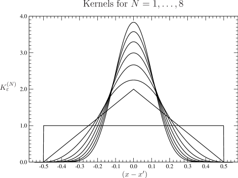
Figure 1: The kernels of the first few lower-order filters with constant range $\varepsilon$, obtained via the use of their Fourier series, for $N=1,\ldots,8$ and $\varepsilon=0.5$, plotted as functions of $\left(x-x^{\prime}\right)$ over their common support within the periodic interval $[-\pi,\pi]$.

so long as $\varepsilon\leq\pi$. Since the range is now constant, one can consider iterations of any order $N$, without any upper bound, even within the periodic interval. Note that this series converges ever faster as $N$ increases. Note also that it can be differentiated $N-2$ times still resulting in a absolutely and uniformly convergent series, and $N-1$ times still resulting in a point-wise convergent series. This is a reflection of the fact that the polynomials that compose the kernel are connected to each other in the maximally smooth way. Apart from the case of the order-zero kernel, which has a divergent Fourier series, the series for $K_{\varepsilon}^{(1)}\!\left(x-x^{\prime}\right)$ is the only one which is not absolutely or uniformly convergent, although it is point-wise convergent. For $N\geq 2$ all the kernel series are absolutely and uniformly convergent to functions of differentiability class $C^{N-2}$ everywhere. The kernels of the filters of the first few orders, with constant range $\varepsilon$, are shown in Figure 1. The program used to plot this graph is available online [4].

As we saw above, the order-$N$ kernels are themselves a good example of the smoothing action of the filters. As we verified in that case, the use of higher-order filters will have the effect of introducing more powers of $k$ in the denominators of the Fourier coefficients $\alpha_{k}$ and $\beta_{k}$, and hence of making the Fourier series converge faster and to smoother functions. This will then enable one to take a certain number of term-wise derivatives of the series, as may be required by the applications involved. Besides, all this can be done within a small constant length scale determined by $\varepsilon$, leaving essentially untouched the description of the physics at the larger scales.

3 Application in Partial Differential Equations

Let us now describe how one can use the low-pass filters in boundary value problems involving partial differential equations. The basic idea is that, if the solution of a boundary value problem leads to a divergent Fourier series for some physical quantity, then the correct physical interpretation of this fact is that the mathematical description of the physical system being dealt with lacks sufficient realism. This is usually a problem contained within the initial conditions used, or within the boundary conditions used, or both. The divergences are always consequences of singularities contained within these conditions. We therefore use the filters in order to smooth out the initial or boundary conditions, using some small range parameter $\varepsilon$ which is suggested by the relevant physical scales of the physical system. Having done that, we may then repeat the whole resolution of the boundary value problem. The solution obtained in this way will then present lesser convergence problems, and quite probably none at all.

While using this technique, it is useful to keep in mind some basic mathematical and physical facts regarding divergences and singularities. There are two basic types of divergence that can happen in a Fourier series, divergence to infinity and indefinite oscillations or endless wandering. If the series diverges everywhere over its periodic domain, then the divergences may occur for two reasons, either there may exist no real function that gives the Fourier coefficients of that series, or there may be a failure of the internal mathematical machinery to represent correctly an existing real function. On the other hand, if there is convergence almost everywhere, and only one or more isolated points of divergence to infinity, then it is likely that the divergences are caused by the real function actually having integrable singularities at these isolated points.

Only very radical divergence at all points within the domain can possibly imply the actual non-existence of a real function that gives the coefficients of the series. This is discussed in [2] and [3], in terms of an analytic structure that leads to a simple and natural classification of divergences and singularities. The typical case would be that in which the coefficients of a trigonometric series diverge exponentially with $k$ when $k\to\infty$, in which case the trigonometric series may fail to be a Fourier series at all. This is seldom the case, so that in general we have either oscillatory divergence almost everywhere, signifying a failure of the internal mathematical machinery to represent faithfully an existing real function, or divergence to infinity at isolated points where the real function being represented by the Fourier series has actual integrable singularities.

In strict physical terms every divergence represents a failure to represent or describe the physical world adequately. This means that either the fundamental physical theory being used has failed, or that the mathematical representation of the particular physical system at hand is inadequate. The latter is much more often the case than the former, with the description of the system being usually either oversimplified or incomplete. For well-established fundamental physical theories being used in a well-established domain of validity, the possibility of a fundamental failure of the theory is an extremely remote one. On the other hand, oversimplification of initial or boundary conditions is a relatively common occurrence.

It is often possible to greatly simplify the use of the filters, avoiding the necessity to solve the boundary value problem all over again after the application of the filter. This is a consequence of the fact that the filter operation often commutes with the differential operator contained within the partial differential equation. In order to see this, let us recall that the first-order filter can be understood as an integral operator, which acts on the space of integrable real functions, since it maps each real function to another real function. Let us show that the elements of the Fourier basis are eigenfunctions of this operator. If we apply the filter as defined in Equation (1) to one of the cosine functions of the basis we get

$$\frac{1}{2\varepsilon}\int_{x-\varepsilon}^{x+\varepsilon}dx^{\prime}\,\cos\!\left(kx^{\prime}\right) = \frac{1}{2\varepsilon k}\sin\!\left(kx^{\prime}\right)\left.\rule{0.0pt}{12.91663pt}\right[_{\,x-\varepsilon}^{\,x+\varepsilon}$$

$$= \frac{1}{2\varepsilon k}\left[\sin(kx+k\varepsilon)-\sin(kx-k\varepsilon)\right]$$

$$= \frac{1}{2\varepsilon k}\left[\sin(kx)\cos(k\varepsilon)+\cos(kx)\sin(k\varepsilon)\right.$$

$$\hskip 20.00003pt-\left.\sin(kx)\cos(k\varepsilon)+\cos(kx)\sin(k\varepsilon)\right]$$

$$= \left[\frac{\sin(k\varepsilon)}{(k\varepsilon)}\right]\cos(kx).$$

This establishes the result, and also determines the eigenvalue, given by the ratio shown within brackets. Once again we see here the sinc function of the variable $(k\varepsilon)$, the same that appears in the Fourier expansions of the kernels. The same can be done for the sine functions, yielding

$$\frac{1}{2\varepsilon}\int_{x-\varepsilon}^{x+\varepsilon}dx^{\prime}\,\sin\!\left(kx^{\prime}\right) = -\,\frac{1}{2\varepsilon k}\cos\!\left(kx^{\prime}\right)\left.\rule{0.0pt}{12.91663pt}\right[_{\,x-\varepsilon}^{\,x+\varepsilon}$$

$$= -\,\frac{1}{2\varepsilon k}\left[\cos(kx+k\varepsilon)-\cos(kx-k\varepsilon)\right]$$

$$= -\,\frac{1}{2\varepsilon k}\left[\cos(kx)\cos(k\varepsilon)-\sin(kx)\sin(k\varepsilon)\right.$$

$$\hskip 30.00005pt-\left.\cos(kx)\cos(k\varepsilon)-\sin(kx)\sin(k\varepsilon)\right]$$

$$= \left[\frac{\sin(k\varepsilon)}{(k\varepsilon)}\right]\sin(kx).$$

Note that this establishes the fact that these are the eigenfunctions of the filter operator for all values of $\varepsilon$ in $(0,\pi)$. In other words, this fact is stable by small variations of the real parameter $\varepsilon$. As one can see, we have here the same eigenvalue as in the previous case. There is therefore a degenerescence between each pair of elements of the basis with the same value of $k$. It is also possible to show that, up to this degenerescence, and assuming the stability by small changes of $\varepsilon$, the elements of the Fourier basis are the only eigenfunctions of the filter operator when defined within the periodic interval, as one can see in Section A.13 of Appendix A. What all this means is that the filter acts in an extremely simple way on the Fourier expansions. If we have the Fourier expansion of the real function $f(x)$ in the periodic interval $[-\pi,\pi]$,

$$f(x)=\frac{1}{2}\,\alpha_{0}+\sum_{k=1}^{\infty}\left[\alpha_{k}\cos(kx)+\beta_{k}\sin(kx)\right],$$

it follows at once that the corresponding expansion for the filtered function is

$$f_{\varepsilon}(x)=\frac{1}{2}\,\alpha_{0}+\sum_{k=1}^{\infty}\left\{\alpha_{k}\left[\frac{\sin(k\varepsilon)}{(k\varepsilon)}\right]\cos(kx)+\beta_{k}\left[\frac{\sin(k\varepsilon)}{(k\varepsilon)}\right]\sin(kx)\right\}.$$

What this means is that the Fourier coefficients $\alpha_{\varepsilon,k}$ and $\beta_{\varepsilon,k}$ of $f_{\varepsilon}(x)$ are given by

$$\alpha_{\varepsilon,k} = \left[\frac{\sin(k\varepsilon)}{(k\varepsilon)}\right]\alpha_{k},$$

$$\beta_{\varepsilon,k} = \left[\frac{\sin(k\varepsilon)}{(k\varepsilon)}\right]\beta_{k},$$

a fact that can be shown directly and independently of the operator-based argument used here, as one can see in Section A.12 of Appendix A. Since the $\sin(k\varepsilon)$ in the numerator of the ratio within brackets is a limited function, while in the denominator we have simply $(k\varepsilon)$, in terms of the asymptotic behavior of the coefficients the inclusion of the ratio, and hence the action of the filter, corresponds simply to the inclusion of a factor of $k$ in the denominator.

Since the elements of the Fourier basis are also eigenfunctions of the second-derivative operator, as one can easily see by simply calculating the derivatives,

$$\frac{\partial^{2}}{\partial x^{2}}\cos(kx) = -k^{2}\cos(kx),$$

$$\frac{\partial^{2}}{\partial x^{2}}\sin(kx) = -k^{2}\sin(kx),$$

we may conclude that within the periodic interval the second-derivative operator and the first-order low-pass filter operator have a complete set of functions as a common set of eigenfunctions. It follows that the two operators commute, a result which can be immediately extended to the higher-order filters. Therefore, given any partial differential equation which is purely second-order on the variable $x$ on which the filter acts, and whose coefficients do not depend on that variable, it follows that if a function $f(x)$ solves the equation, then the filtered function $f_{\varepsilon}(x)$ is also a solution.

This leads to the fact that one may apply the filter directly to the solution of the unfiltered problem, thus obtaining the same result that one would obtain by first applying the filter to the initial or boundary conditions and then solving the boundary value problem all over again. This is the case for the Laplace equation, the wave equation and the diffusion equation, in either Cartesian or cylindrical coordinates. Since the unfiltered solution is represented in terms of a (possibly divergent) Fourier series, in such circumstances it is immediate to write down the filtered solution, by simply plugging the filter factor given by the sinc function into the coefficients of the Fourier series obtained in the usual way, as is illustrated by the examples in Appendix B. Since it usually takes much more work to solve the boundary value problem with the filtered initial or boundary conditions than to solve the corresponding unfiltered problem, this can save a lot of work and effort.

4 Conclusions

Linear low-pass filters of arbitrary orders can be easily defined on the real line, in a very simple way, either on the whole line or within a periodic interval. We presented a definition of such filters in precise mathematical terms, and also wrote them as linear integral operators acting in the space of integrable real functions, expressed as integrals involving certain kernel functions. We established several of the main properties of the first-order filter. Due to the linearity of the filters some of these properties, those involving the concept of invariance, are immediately generalizable to the higher-order filters.

The use of the filters on divergent Fourier series produces other series which are convergent, but which remain closely related to the original problem within the physics application being dealt with, so long as the range $\varepsilon$ is sufficiently small. It also produces series that converge faster to smoother functions, and that can be differentiated a certain number of times, as required by the applications involved, without resulting in divergent series. We thus acquire a useful set of tools to deal with Fourier series in a way that has a clear physical meaning in the context of applications in physics. This set of tools can then be used as a probe into the physical structure of the problems being dealt with.

It also follows in a very simple way that the filter operators commute with the second derivative operator. We showed this in the case of the first-order filter, and since the higher-order filters are just the first-order one applied successive times, the result is immediately extended to them. This leads to the fact that in many cases one may obtain the solutions of the filtered boundary valuer problems by the simple application of the filters directly to the solutions of the unfiltered problems. This is very easily done when the solutions are expressed as Fourier series, and may greatly simplify matters in practice.

Since any limited integrable function will have a limited set of Fourier coefficients, it suffices to apply to such functions the first-order linear low-pass filter of range $\varepsilon$ twice, or the second-order filter of range $\varepsilon$ just once, in order to ensure the absolute and uniform convergence of the resulting Fourier series. Therefore, it becomes clear that any divergence of the original series must be due to detailed structure that exists below the length scale that characterizes these filters. For small enough values of the range of the filters such structure cannot have a bearing on the physics involved, which allows us to use the filters in this way. But besides this practical application the filters give us a simple, clear and intuitive way to understand the origin of the eventual divergences of the Fourier series.

5 Acknowledgements

The author would like to thank his friend and colleague Prof. Carlos Eugênio Imbassay Carneiro, to whom he is deeply indebted for all his interest and help, as well as his careful reading of the manuscript and helpful criticism regarding this work.

Appendix A Appendix: Properties of the First-Order Filter

Here we present simple proofs of the main properties of the first-order linear low-pass filter on the real line of the coordinate $x$.

A.1 Invariance of Linear Functions

Let us show that if $f(x)$ is a linear function on the real line, then $f_{\varepsilon}(x)=f(x)$. It suffices to simply calculate $f_{\varepsilon}(x)$. We have $f(x)=a+bx$, so that

$$f_{\varepsilon}(x) = \frac{1}{2\varepsilon}\int_{x-\varepsilon}^{x+\varepsilon}dx^{\prime}\,\left(a+bx^{\prime}\right)$$

$$= \frac{1}{2\varepsilon}\left(ax^{\prime}+b\,\frac{x^{\prime 2}}{2}\right)\left.\rule{0.0pt}{12.91663pt}\right[_{\,x-\varepsilon}^{\,x+\varepsilon}$$

$$= \frac{1}{2\varepsilon}\left[a\left(x+\varepsilon-x+\varepsilon\right)+b\left(\frac{x^{2}+2x\varepsilon+\varepsilon^{2}}{2}-\frac{x^{2}-2x\varepsilon+\varepsilon^{2}}{2}\right)\right]$$

$$= \frac{1}{2\varepsilon}\left(2a\varepsilon+2bx\varepsilon\right)$$

$$= a+2bx$$

$$= f(x).$$

Note that if a function is defined in a piece-wise fashion, in any section where it is linear the filter is the identity at all points $x$ where the interval $(x-\varepsilon,x+\varepsilon)$ fits completely inside the section. Therefore, in the $\varepsilon\to 0$ limit the filter becomes the identity in the whole interior of such a section.

A.2 Action on Powers and Polynomials

Let us determine the action of the filter on a function which is a simple power on the real line. If $f(x)=x^{n}$ then we have

$$f_{\varepsilon}(x) = \frac{1}{2\varepsilon}\int_{x-\varepsilon}^{x+\varepsilon}dx\,x^{\prime n}$$

$$= \frac{1}{2\varepsilon(n+1)}\,x^{\prime(n+1)}\left.\rule{0.0pt}{12.91663pt}\right[_{\,x-\varepsilon}^{\,x+\varepsilon}$$

$$= \frac{1}{2\varepsilon(n+1)}\left[(x+\varepsilon)^{n+1}-(x-\varepsilon)^{n+1}\right]$$

$$= \frac{1}{2\varepsilon(n+1)}\sum_{k=0}^{n+1}\frac{(n+1)!}{k!(n+1-k)!}\,x^{n+1-k}\varepsilon^{k}\left[1-(-1)^{k}\right]$$

$$= \frac{1}{\varepsilon(n+1)}\sum_{j=0}^{j_{M}}\frac{(n+1)!}{k!(n+1-k)!}\,x^{n+1-k}\varepsilon^{k},$$

where $k=2j+1$ and $j_{M}=n/2$ if $n$ is even, while $j_{M}=(n-1)/2$ if $n$ is odd. We have therefore

$$f_{\varepsilon}(x) = \sum_{j=0}^{j_{M}}\frac{n!\varepsilon^{2j}}{(2j+1)!(n-2j)!}\,x^{n-2j}$$

$$= x^{n}+\frac{n(n-1)\varepsilon^{2}}{3!}\,x^{n-2}+\frac{n(n-1)(n-2)(n-3)\varepsilon^{4}}{5!}\,x^{n-4}+\ldots\;.$$

We see therefore that the filter preserves the original power, and that all other terms generated are of lower order and are damped by factors of $\varepsilon^{2}$. It follows that the filter will reproduce any order-$n$ polynomial, adding to it a lower-order polynomial, of order $n-2$, with all coefficients damped by powers of $\varepsilon^{2}$. Therefore, in the $\varepsilon\to 0$ limit the filter reduces to the identity, in so far as polynomials are concerned.

A.3 Differentiability of Filtered Functions

Let us show that for any continuous function $f(x)$ the filtered function $f_{\varepsilon}(x)$ is differentiable. We simply calculate the filtered function $f_{\varepsilon}(x)$ at $x$ and $x+\Delta x$, then calculate its variation $\Delta f_{\varepsilon}(x)$, divide by $\Delta x$ and finally make $\Delta x\to 0$. The finite-difference ratio is given by

$$\frac{\Delta f_{\varepsilon}(x)}{\Delta x} = \frac{f_{\varepsilon}(x+\Delta x)-f_{\varepsilon}(x)}{\Delta x}$$

$$= \frac{1}{2\varepsilon\Delta x}\int_{x+\Delta x-\varepsilon}^{x+\Delta x+\varepsilon}dx^{\prime}\,f\!\left(x^{\prime}\right)-\frac{1}{2\varepsilon\Delta x}\int_{x-\varepsilon}^{x+\varepsilon}dx^{\prime}\,f\!\left(x^{\prime}\right).$$

For any given value of $\varepsilon$, in the $\Delta x\to 0$ limit we will eventually have $\Delta x\ll\varepsilon$, and then the domains of the two integrals overlap in most of their extent, which we can see decomposing the integrals as

$$\frac{\Delta f_{\varepsilon}(x)}{\Delta x} = \frac{1}{2\varepsilon\Delta x}\int_{x+\Delta x-\varepsilon}^{x+\varepsilon}dx^{\prime}\,f\!\left(x^{\prime}\right)+\frac{1}{2\varepsilon\Delta x}\int_{x+\varepsilon}^{x+\Delta x+\varepsilon}dx^{\prime}\,f\!\left(x^{\prime}\right)+$$

$$-\,\frac{1}{2\varepsilon\Delta x}\int_{x-\varepsilon}^{x+\Delta x-\varepsilon}dx^{\prime}\,f\!\left(x^{\prime}\right)-\frac{1}{2\varepsilon\Delta x}\int_{x+\Delta x-\varepsilon}^{x+\varepsilon}dx^{\prime}\,f\!\left(x^{\prime}\right)$$

$$= \frac{1}{2\varepsilon}\left[\frac{1}{\Delta x}\int_{(x+\varepsilon)}^{(x+\varepsilon)+\Delta x}dx^{\prime}\,f\!\left(x^{\prime}\right)\right]-\frac{1}{2\varepsilon}\left[\frac{1}{\Delta x}\int_{(x-\varepsilon)}^{(x-\varepsilon)+\Delta x}dx^{\prime}\,f\!\left(x^{\prime}\right)\right].$$

We have here two integrals over intervals of length $\Delta x$, divided by $\Delta x$. These normalized integrals give therefore the average values of $f(x)$ around the points $x+\varepsilon$ and $x-\varepsilon$. Since the function $f(x)$ is integrable these average values are finite, and since it is continuous, the average value tends to the value of the function when $\Delta x\to 0$, so that we get

$$\lim_{\Delta x\to 0}\frac{\Delta f_{\varepsilon}(x)}{\Delta x}=\frac{f\!\left(x+\varepsilon\right)-f\!\left(x-\varepsilon\right)}{2\varepsilon}.$$

This is true both for positive and negative values of $\Delta x$, and the limit manifestly exists and has the value shown, which is independent of the sign of $\Delta x$. Therefore, this establishes that $f_{\varepsilon}(x)$ is differentiable.

A.4 Continuity of Filtered Functions

Let us show that for any integrable function $f(x)$ the filtered function $f_{\varepsilon}(x)$ is continuous. We simply calculate the filtered function at $x$ and $x+\Delta x$ and then make $\Delta x\to 0$. The variation of $f_{\varepsilon}(x)$ is given by

$$\Delta f_{\varepsilon}(x) = f_{\varepsilon}(x+\Delta x)-f_{\varepsilon}(x)$$

$$= \frac{1}{2\varepsilon}\int_{x+\Delta x-\varepsilon}^{x+\Delta x+\varepsilon}dx^{\prime}\,f\!\left(x^{\prime}\right)-\frac{1}{2\varepsilon}\int_{x-\varepsilon}^{x+\varepsilon}dx^{\prime}\,f\!\left(x^{\prime}\right).$$

For any given value of $\varepsilon$, in the $\Delta x\to 0$ limit we will eventually have $\Delta x\ll\varepsilon$, and then the domains of the two integrals overlap in most of their extent, which we can see decomposing the integrals as

$$\Delta f_{\varepsilon}(x) = \frac{1}{2\varepsilon}\int_{x+\Delta x-\varepsilon}^{x+\varepsilon}dx^{\prime}\,f\!\left(x^{\prime}\right)+\frac{1}{2\varepsilon}\int_{x+\varepsilon}^{x+\Delta x+\varepsilon}dx^{\prime}\,f\!\left(x^{\prime}\right)+$$

$$-\,\frac{1}{2\varepsilon}\int_{x-\varepsilon}^{x+\Delta x-\varepsilon}dx^{\prime}\,f\!\left(x^{\prime}\right)-\frac{1}{2\varepsilon}\int_{x+\Delta x-\varepsilon}^{x+\varepsilon}dx^{\prime}\,f\!\left(x^{\prime}\right)$$

$$= \frac{1}{2\varepsilon}\left[\int_{(x+\varepsilon)}^{(x+\varepsilon)+\Delta x}dx^{\prime}\,f\!\left(x^{\prime}\right)\right]-\frac{1}{2\varepsilon}\left[\int_{(x-\varepsilon)}^{(x-\varepsilon)+\Delta x}dx^{\prime}\,f\!\left(x^{\prime}\right)\right].$$

We have here two integrals over intervals of length $\Delta x$. In the $\Delta x\to 0$ limit we have integrals over zero-measure domains, and since the function $f(x)$ is integrable, the result is zero,

$$\lim_{\Delta x\to 0}\Delta f_{\varepsilon}(x)=0,$$

regardless of the sign of $\Delta x$, which establishes that $f_{\varepsilon}(x)$ is continuous.

A.5 Action on Dirac’s Delta “Function”

Let us assume that we have the “function” $f(x)=\delta(x-x_{0})$. Since this is an integrable object, we may calculate the corresponding filtered function, which as we shall see is in fact an actual function. The function $f_{\varepsilon}(x)$ that corresponds to $f(x)$ through the first-order filter of range $\varepsilon$ is, by definition,

$$f_{\varepsilon}(x)=\frac{1}{2\varepsilon}\int_{x-\varepsilon}^{x+\varepsilon}dx^{\prime}\,\delta(x^{\prime}-x_{0}).$$

By the properties of the delta “function”, this integral will be equal to $1$ if the point $x_{0}$ is within the integration interval, and $0$ if it is outside. The point $x_{0}$ can only be within the integration interval if the distance between $x$ and $x_{0}$ is smaller than $\varepsilon$, that is, if $|x-x_{0}|<\varepsilon$. Therefore we have for the resulting function the piece-wise description

$$\begin{array}[]{rclcl}f_{\varepsilon}(x)&=&0&\mbox{if}&x<(x_{0}-\varepsilon),\\ f_{\varepsilon}(x)&=&{\displaystyle\frac{\displaystyle 1}{\displaystyle 2\varepsilon}}&\mbox{if}&(x_{0}-\varepsilon)<x<(x_{0}+\varepsilon),\\ f_{\varepsilon}(x)&=&0&\mbox{if}&(x_{0}+\varepsilon)<x.\end{array}$$

This is a rectangular pulse centered at $x_{0}$, with height $1/(2\varepsilon)$ and width $(2\varepsilon)$, having therefore unit area. Note that this is, in fact, the first-order kernel itself, that is

$$f_{\varepsilon}(x)=K_{\varepsilon}^{(1)}(x-x_{0}).$$

This one-parameter family of functions is one that is commonly used for the very definition the Dirac delta “function” in the limit $\varepsilon\to 0$, and therefore we have that

$$\lim_{\varepsilon\to 0}K_{\varepsilon}^{(1)}(x-x_{0})=\delta(x-x_{0}).$$

Looking at the filter as an operator in some larger space of integrable objects, this means that it becomes the identity in the $\varepsilon\to 0$ limit, in so far as delta “functions” are concerned. Note that the delta “function” can also be understood as the kernel of an order-zero filter,

$$f_{0}^{(0)}(x)=\int_{-\infty}^{\infty}dx^{\prime}\,\delta\!\left(x-x^{\prime}\right)f\!\left(x^{\prime}\right).$$

This filter is the identity where $f(x)$ is continuous, so that typically it is the identity almost everywhere. Note also that, as a particular case of this expression, we may conclude that the first-order kernel is the result of the application of the first-order filter to the delta “functions”,

$$K_{\varepsilon}^{(1)}\!\left(x-x^{\prime\prime}\right)=\int_{-\infty}^{\infty}dx^{\prime}\,K_{\varepsilon}^{(1)}\!\left(x^{\prime}-x^{\prime\prime}\right)\delta\!\left(x-x^{\prime}\right),$$

which holds everywhere so long as the first-order kernel is defined as we did in Equation (2) and so long as we use the average of the two lateral limits as the value given by the integral of the delta “function” at a point of discontinuity of the function involved.

A.6 Reduction to the Identity

Let us show that in the $\varepsilon\to 0$ limit the filter reduces to an almost-identity operation, in the sense that it reproduces in the output function $f_{\varepsilon}(x)$ the input function $f(x)$ almost everywhere. If we consider the well-known relation mentioned in the previous section as a possible definition of the Dirac delta “function”, as the $\varepsilon\to 0$ limit of the first-order kernel $K_{\varepsilon}^{(1)}\!\left(x-x^{\prime}\right)$, it becomes clear that we have, for an arbitrary integrable function $f(x)$

$$\lim_{\varepsilon\to 0}f_{\varepsilon}(x) = \lim_{\varepsilon\to 0}\int_{-\infty}^{\infty}dx^{\prime}\,K_{\varepsilon}^{(1)}\!\left(x-x^{\prime}\right)f\!\left(x^{\prime}\right)$$

$$= \int_{-\infty}^{\infty}dx^{\prime}\,\left[\,\lim_{\varepsilon\to 0}K_{\varepsilon}^{(1)}\!\left(x-x^{\prime}\right)\right]f\!\left(x^{\prime}\right)$$

$$= \int_{-\infty}^{\infty}dx^{\prime}\,\delta(x-x^{\prime})f\!\left(x^{\prime}\right).$$

According to the properties of the delta “function”, this integral returns the value $f(x)$ at every point where this function is continuous. We therefore have

$$\lim_{\varepsilon\to 0}f_{\varepsilon}(x)=f(x),$$

at every point where $f(x)$ is continuous. Since this may fail at a finite (or at least zero-measure) set of points where $f(x)$ is discontinuous, we say that in the $\varepsilon\to 0$ limit the first-order filter reduces to the identity almost everywhere. We may also say that the filter becomes an almost-identity operation in the limit. What happens at the points of discontinuity of $f(x)$ is discussed in the next section.

A.7 Points of Discontinuity

Let us show that in the $\varepsilon\to 0$ limit the function $f_{\varepsilon}(x)$ essentially reproduces the original function $f(x)$. Stating it more precisely, we will show that, if the function $f(x)$ has an isolated point of discontinuity at $x_{0}$, then in the $\varepsilon\to 0$ limit $f_{\varepsilon}(x_{0})$ tends to the average of the two lateral limits of $f(x)$ to the point $x_{0}$, that is,

$$\lim_{\varepsilon\to 0}f_{\varepsilon}(x_{0})=\frac{1}{2}\left({\cal L}_{+}+{\cal L}_{-}\right),$$

where

$${\cal L}_{\pm}=\lim_{x\to x_{0\pm}}f(x),$$

regardless of the value that $f(x)$ assumes at $x_{0}$. In particular, if $f(x)$ is continuous at $x_{0}$, then ${\cal L}_{+}={\cal L}_{-}=f(x_{0})$ and hence $f_{\varepsilon}(x_{0})$ tends to $f(x_{0})$ in the limit, thus reproducing the original function at that point.

Here is the proof: if $f(x)$ has an isolated point of discontinuity at $x_{0}$, then there are two neighborhoods of $x_{0}$, one to the left and another one to the right, where $f(x)$ is continuous. For sufficiently small $\varepsilon$, the interval of integration will fit into this combined neighborhood, so that the only point of discontinuity within it will be $x_{0}$. Let us consider then the value of $f_{\varepsilon}(x_{0})$, as given by the definition,

$$f_{\varepsilon}(x_{0})=\frac{1}{2\varepsilon}\int_{x_{0}-\varepsilon}^{x_{0}+\varepsilon}dx^{\prime}\,f(x^{\prime}).$$

We may separate this integral in two, one in the left neighborhood and another one in the right neighborhood,

$$f_{\varepsilon}(x_{0})=\frac{1}{2\varepsilon}\int_{x_{0}-\varepsilon}^{x_{0}}dx^{\prime}\,f(x^{\prime})+\frac{1}{2\varepsilon}\int_{x_{0}}^{x_{0}+\varepsilon}dx^{\prime}\,f(x^{\prime}).$$

Since the function $f(x)$ is integrable, the integrals converge to $\varepsilon$ times the average value of the function over each sub-interval, so that we have

$$\lim_{\varepsilon\to 0}f_{\varepsilon}(x_{0})=\frac{1}{2}\bar{f}(x_{0-})+\frac{1}{2}\bar{f}(x_{0+}).$$

Finally, since the function $f(x)$ is continuous in each sub-interval, in the $\varepsilon\to 0$ limit each average value converges to the corresponding lateral limit of $f(x)$, so that we have

$$\lim_{\varepsilon\to 0}f_{\varepsilon}(x_{0})=\frac{1}{2}\left({\cal L}_{+}+{\cal L}_{-}\right),$$

where

$${\cal L}_{\pm}=\lim_{x\to x_{0\pm}}f(x).$$

This establishes the result. As a consequence of this, if $f(x)$ is continuous at $x_{0}$, then ${\cal L}_{+}={\cal L}_{-}=f(x_{0})$, and therefore we have

$$\lim_{\varepsilon\to 0}f_{\varepsilon}(x_{0})=f(x_{0}).$$

We therefore conclude that in the $\varepsilon\to 0$ limit the filtered function $f_{\varepsilon}(x)$ reproduces the original function $f(x)$ where it is continuous. There may be isolated points of discontinuity where this fails, and therefore we say that in the $\varepsilon\to 0$ limit the filtered function $f_{\varepsilon}(x)$ reproduces the original function $f(x)$ almost everywhere.

A.8 Points of Non-Differentiability

Let us show that in the $\varepsilon\to 0$ limit the derivative of the function $f_{\varepsilon}(x)$ essentially reproduces the derivative of the original function $f(x)$. Stating it more precisely, we will show that, if the function $f(x)$ is continuous but has an isolated point of non-differentiability at $x_{0}$, then in the $\varepsilon\to 0$ limit the derivative of $f_{\varepsilon}(x_{0})$ tends to the average of the two lateral limits of the derivative of $f(x)$ to the point $x_{0}$, that is,

$$\lim_{\varepsilon\to 0}\frac{df_{\varepsilon}}{dx}(x_{0})=\frac{1}{2}\left({\cal L^{\prime}}_{+}+{\cal L^{\prime}}_{-}\right),$$

where

$${\cal L^{\prime}}_{\pm}=\lim_{x\to x_{0\pm}}\frac{df}{dx}(x),$$

regardless of any value that may be artificially given to the derivative of $f(x)$ at $x_{0}$. In particular, if $f(x)$ is differentiable at $x_{0}$, then ${\cal L^{\prime}}_{+}$ and ${\cal L^{\prime}}_{-}$ are both equal to the derivative of $f(x)$ at $x_{0}$, and hence the derivative of $f_{\varepsilon}(x)$ tends to the derivative of $f(x)$ at $x_{0}$ in the limit, thus reproducing the derivative of the original function at that point.

Here is the proof: if $f(x)$ is continuous at $x_{0}$ and has an isolated point of discontinuity there, then there are two neighborhoods of $x_{0}$, one to the left and another one to the right, where $f(x)$ is continuous and differentiable. According to the results of Section A.3 of this Appendix, since $f(x)$ is continuous at and around $x_{0}$, $f_{\varepsilon}(x)$ is differentiable and its derivative at $x_{0}$ is given by

$$\frac{df_{\varepsilon}}{dx}(x_{0})=\frac{f(x_{0}+\varepsilon)-f(x_{0}-\varepsilon)}{2\varepsilon}.$$

However, since $f(x)$ is not differentiable at $x_{0}$, the $\varepsilon\to 0$ limit of the right-hand side of this equation does not give us any definite results. We may however separate this expression in two, each one making reference to only one of the two neighborhoods,

$$\frac{df_{\varepsilon}}{dx}(x_{0}) = \frac{f(x_{0}+\varepsilon)-f\!\left(x_{0}\right)+f\!\left(x_{0}\right)-f(x_{0}-\varepsilon)}{2\varepsilon}$$

$$= \frac{1}{2}\,\frac{f(x_{0}+\varepsilon)-f(x_{0})}{\varepsilon}+\frac{1}{2}\,\frac{f(x_{0})-f(x_{0}-\varepsilon)}{\varepsilon}.$$

It is now clear that, since $f(x)$ is differentiable in the two lateral neighborhoods, in the $\varepsilon\to 0$ limit the two terms in the right-hand side of this equation converge respectively to the right and left derivatives of $f(x)$ at $x_{0}$. We therefore have

$$\lim_{\varepsilon\to 0}\frac{df_{\varepsilon}}{dx}(x_{0})=\frac{1}{2}\left({\cal L^{\prime}}_{+}+{\cal L^{\prime}}_{-}\right),$$

where

$${\cal L^{\prime}}_{\pm}=\lim_{x\to x_{0\pm}}\frac{df}{dx}(x).$$

This establishes the result. In particular, if $f(x)$ is differentiable at $x_{0}$, then ${\cal L^{\prime}}_{+}$ and ${\cal L^{\prime}}_{-}$ are both equal to the derivative of $f(x)$ at $x_{0}$, and therefore we have for the derivative of $f_{\varepsilon}(x)$ at $x_{0}$

$$\lim_{\varepsilon\to 0}\frac{df_{\varepsilon}}{dx}(x_{0})=\frac{df}{dx}(x_{0}),$$

thus reproducing the derivative of the original function at that point.

A.9 Invariance of Definite Integrals

Let us determine the effect of the filter on the definite integral of a function $f(x)$ with compact support on the real line. We may write the integral as

$$I=\int_{-\infty}^{\infty}dx\,f(x),$$

where the integrand is non-zero only inside a closed interval. The integral of the filtered function $f_{\varepsilon}(x)$ has support on another closed interval, that of $f(x)$ increased by $\varepsilon$ in each direction, and is similarly given by

$$I_{\varepsilon} = \int_{-\infty}^{\infty}dx\,f_{\varepsilon}(x)$$

$$= \int_{-\infty}^{\infty}dx\,\frac{1}{2\varepsilon}\int_{x-\varepsilon}^{x+\varepsilon}dx^{\prime}\,f\!\left(x^{\prime}\right)$$

$$= \frac{1}{2\varepsilon}\int_{-\infty}^{\infty}dx\,\int_{x-\varepsilon}^{x+\varepsilon}dx^{\prime}\,f\!\left(x^{\prime}\right),$$

where we used the definition of $f_{\varepsilon}(x)$ in terms of $f(x)$. We now make the change of variables $x^{\prime}=x^{\prime\prime}+x$ on the inner integral, implying $dx^{\prime}=dx^{\prime\prime}$ and $x^{\prime\prime}=x^{\prime}-x$, leading to

$$I_{\varepsilon} = \frac{1}{2\varepsilon}\int_{-\infty}^{\infty}dx\,\int_{-\varepsilon}^{\varepsilon}dx^{\prime\prime}\,f(x^{\prime\prime}+x),$$

$$= \frac{1}{2\varepsilon}\int_{-\varepsilon}^{\varepsilon}dx^{\prime\prime}\,\int_{-\infty}^{\infty}dx\,f(x^{\prime\prime}+x).$$

Since the integral on $x$ is over the whole real line, we may now change variables on it without changing the integration limits, using $x=x^{\prime}-x^{\prime\prime}$, with $x^{\prime}=x^{\prime\prime}+x$ and $dx=dx^{\prime}$, and thus obtaining

$$I_{\varepsilon} = \frac{1}{2\varepsilon}\int_{-\varepsilon}^{\varepsilon}dx^{\prime\prime}\,\int_{-\infty}^{\infty}dx^{\prime}\,f\!\left(x^{\prime}\right)$$

$$= \frac{1}{2\varepsilon}\int_{-\varepsilon}^{\varepsilon}dx^{\prime\prime}\,I$$

$$= I,$$

were we recognized the form of the integral $I$. In this way we show that $I_{\varepsilon}=I$, that is, the filter does not change the definite integral at all. Another way to state this is to say that the filter does not change the average value of $f(x)$ over the common support of $f(x)$ and $f_{\varepsilon}(x)$.

A.10 Periodicity of Filtered Functions

Let us show that if $f(x)$ is a periodic function, with a period that we choose arbitrarily to be $2\pi$, then $f_{\varepsilon}(x)$ is also periodic, with the same period. It suffices to simply calculate

$$f_{\varepsilon}(x+2\pi) = \frac{1}{2\varepsilon}\int_{x+2\pi-\varepsilon}^{x+2\pi+\varepsilon}dx^{\prime}\,f\!\left(x^{\prime}\right)$$

$$= \frac{1}{2\varepsilon}\int_{x-\varepsilon}^{x+\varepsilon}dx^{\prime\prime}\,f\!\left(x^{\prime\prime}+2\pi\right),$$

where we changed variables to $x^{\prime\prime}=x^{\prime}-2\pi$, so that $x^{\prime}=x^{\prime\prime}+2\pi$. Since $f(x)$ is periodic with period $2\pi$, we now have

$$f_{\varepsilon}(x+2\pi) = \frac{1}{2\varepsilon}\int_{x-\varepsilon}^{x+\varepsilon}dx^{\prime\prime}\,f\!\left(x^{\prime\prime}\right)$$

$$= f_{\varepsilon}(x),$$

so that we may conclude that $f_{\varepsilon}(x)$ is periodic with period $2\pi$.

A.11 Invariance of Averages Over the Period

Let us determine the effect of the filter on the Fourier coefficient $\alpha_{0}$. We start with the coefficient of $f(x)$, which is given by

$$\alpha_{0}=\frac{1}{\pi}\int_{-\pi}^{\pi}dx\,f(x),$$

where we arbitrarily chose $[-\pi,\pi]$ as the periodic interval. The Fourier coefficient $\alpha_{\varepsilon,0}$ of $f_{\varepsilon}(x)$ is similarly given by

$$\alpha_{\varepsilon,0} = \frac{1}{\pi}\int_{-\pi}^{\pi}dx\,f_{\varepsilon}(x)$$

$$= \frac{1}{\pi}\int_{-\pi}^{\pi}dx\,\frac{1}{2\varepsilon}\int_{x-\varepsilon}^{x+\varepsilon}dx^{\prime}\,f\!\left(x^{\prime}\right)$$

$$= \frac{1}{2\varepsilon\pi}\int_{-\pi}^{\pi}dx\,\int_{x-\varepsilon}^{x+\varepsilon}dx^{\prime}\,f\!\left(x^{\prime}\right),$$

where we used the definition of $f_{\varepsilon}(x)$ in terms of $f(x)$. We now make the change of variables $x^{\prime}=x^{\prime\prime}+x$ on the inner integral, implying $dx^{\prime}=dx^{\prime\prime}$ and $x^{\prime\prime}=x^{\prime}-x$, leading to

$$\alpha_{\varepsilon,0} = \frac{1}{2\varepsilon\pi}\int_{-\pi}^{\pi}dx\,\int_{-\varepsilon}^{\varepsilon}dx^{\prime\prime}\,f(x^{\prime\prime}+x),$$

$$= \frac{1}{2\varepsilon}\int_{-\varepsilon}^{\varepsilon}dx^{\prime\prime}\,\frac{1}{\pi}\int_{-\pi}^{\pi}dx\,f(x^{\prime\prime}+x).$$

Since the integral on $x$ is over the whole period, we may now change variables on it without changing the integration limits, using $x=x^{\prime}-x^{\prime\prime}$, with $x^{\prime}=x^{\prime\prime}+x$ and $dx=dx^{\prime}$, and thus obtaining

$$\alpha_{\varepsilon,0} = \frac{1}{2\varepsilon}\int_{-\varepsilon}^{\varepsilon}dx^{\prime\prime}\,\frac{1}{\pi}\int_{-\pi}^{\pi}dx^{\prime}\,f\!\left(x^{\prime}\right)$$

$$= \frac{1}{2\varepsilon}\int_{-\varepsilon}^{\varepsilon}dx^{\prime\prime}\,\alpha_{0}$$

$$= \alpha_{0},$$

were we recognized the form of $\alpha_{0}$. In this way we show that $\alpha_{\varepsilon,0}=\alpha_{0}$, that is, the filter does not change $\alpha_{0}$ at all. Another way to state this is to say that the filter does not change the average value of $f(x)$ over the periodic interval.

A.12 Action on the Fourier Coefficients with $k>0$

Let us determine the effect of the filter on the Fourier coefficients for $k>0$. We start with the Fourier coefficients of $f(x)$, which are given by

$$\alpha_{k} = \frac{1}{\pi}\int_{-\pi}^{\pi}dx\,f(x)\cos(kx),$$

$$\beta_{k} = \frac{1}{\pi}\int_{-\pi}^{\pi}dx\,f(x)\sin(kx),$$

where we arbitrarily chose $[-\pi,\pi]$ as the periodic interval. The Fourier coefficients of $f_{\varepsilon}(x)$ are similarly given by

$$\alpha_{\varepsilon,k} = \frac{1}{\pi}\int_{-\pi}^{\pi}dx\,f_{\varepsilon}(x)\cos(kx),$$

$$\beta_{\varepsilon,k} = \frac{1}{\pi}\int_{-\pi}^{\pi}dx\,f_{\varepsilon}(x)\sin(kx).$$

Let us work out only the first case, since the work for the second one in essentially identical. Using the definition of $f_{\varepsilon}(x)$ in terms of $f(x)$ we have

$$\alpha_{\varepsilon,k} = \frac{1}{\pi}\int_{-\pi}^{\pi}dx\,\cos(kx)\,\frac{1}{2\varepsilon}\int_{x-\varepsilon}^{x+\varepsilon}dx^{\prime}\,f\!\left(x^{\prime}\right)$$

$$= -\,\frac{1}{2\varepsilon\pi}\int_{-\pi}^{\pi}dx\,\frac{\sin(kx)}{k}\,\frac{d}{dx}\int_{x-\varepsilon}^{x+\varepsilon}dx^{\prime}\,f\!\left(x^{\prime}\right)$$

$$= -\,\frac{1}{2\varepsilon\pi k}\int_{-\pi}^{\pi}dx\,\sin(kx)\;f\!\left(x^{\prime}\right)\left.\rule{0.0pt}{12.91663pt}\right[_{\,x-\varepsilon}^{\,x+\varepsilon}$$

$$= -\,\frac{1}{2\varepsilon\pi k}\int_{-\pi}^{\pi}dx\,\sin(kx)f(x+\varepsilon)+\frac{1}{2\varepsilon\pi k}\int_{-\pi}^{\pi}dx\,\sin(kx)f(x-\varepsilon),$$

where we integrated by parts and where there is no integrated term due to the periodicity of the integrand on the domain. We now change variables in each integral, using $x^{\prime}=x\pm\varepsilon$, in order to obtain

$$\alpha_{\varepsilon,k} = -\,\frac{1}{2\varepsilon\pi k}\int_{-\pi}^{\pi}dx^{\prime}\,\sin(kx^{\prime}-k\varepsilon)f\!\left(x^{\prime}\right)+\frac{1}{2\varepsilon\pi k}\int_{-\pi}^{\pi}dx^{\prime}\,\sin(kx^{\prime}+k\varepsilon)f\!\left(x^{\prime}\right)$$

$$= \frac{1}{2\varepsilon\pi k}\int_{-\pi}^{\pi}dx^{\prime}\,f\!\left(x^{\prime}\right)\left[\sin(kx^{\prime}+k\varepsilon)-\sin(kx^{\prime}-k\varepsilon)\right],$$

where the integration limits did not change in the transformations of variables due to the periodicity of the integrand on the domain. We are left with

$$\alpha_{\varepsilon,k} = \frac{1}{2\varepsilon\pi k}\int_{-\pi}^{\pi}dx^{\prime}\,f\!\left(x^{\prime}\right)\left[\sin\!\left(kx^{\prime}\right)\cos(k\varepsilon)+\sin(k\varepsilon)\cos\!\left(kx^{\prime}\right)\right.+$$

$$\hskip 90.00014pt-\left.\sin\!\left(kx^{\prime}\right)\cos(k\varepsilon)+\sin(k\varepsilon)\cos\!\left(kx^{\prime}\right)\right]$$

$$= \left[\frac{\sin(k\varepsilon)}{(k\varepsilon)}\right]\frac{1}{\pi}\int_{-\pi}^{\pi}dx^{\prime}\,f\!\left(x^{\prime}\right)\cos\!\left(kx^{\prime}\right).$$

Since we recover in this way the expression of the Fourier coefficients $\alpha_{k}$ of $f(x)$, we get

$$\alpha_{\varepsilon,k}=\left[\frac{\sin(k\varepsilon)}{(k\varepsilon)}\right]\alpha_{k},$$

and repeating the calculation for the other coefficients one gets

$$\beta_{\varepsilon,k}=\left[\frac{\sin(k\varepsilon)}{(k\varepsilon)}\right]\beta_{k}.$$

Once again we see the sinc function of the variable $(k\varepsilon)$ appearing here. Since $\sin(k\varepsilon)$ is a limited function, in terms of the asymptotic behavior of the coefficients, for large values of $k$, the net effect of the filter is to add a factor of $k$ to the denominator.

A.13 Completeness of the Set of Eigenfunctions

Let us show that, up to the degeneracy between the pairs of elements of the basis with the same $k$, the elements of the Fourier basis are the only eigenfunctions of the filter operator, when it is defined within the periodic interval. In order to do this, let us first point out that two eigenvalues, for two different values of $k$, are never equal. We can see this assuming that there are positive values $k$ and $k^{\prime}$ such that

$$\frac{\sin(k\varepsilon)}{(k\varepsilon)}=\frac{\sin\!\left(k^{\prime}\varepsilon\right)}{\left(k^{\prime}\varepsilon\right)}.$$

Since this must stay valid for small changes of $\varepsilon$, we may differentiate with respect to $\varepsilon$ and thus obtain

$$\cos(k\varepsilon)=\cos\!\left(k^{\prime}\varepsilon\right).$$

This now implies that

$$\sin(k\varepsilon)=\pm\sin\!\left(k^{\prime}\varepsilon\right).$$

Since $\varepsilon>0$ and both $k$ and $k^{\prime}$ are positive, we must have

$$\sin(k\varepsilon)=\sin\!\left(k^{\prime}\varepsilon\right).$$

Since both the cosines and the sines of the two arguments are thus seen to be equal, it follows that the two arguments must be equal, and hence that we must have $k=k^{\prime}$. Therefore, the eigenvalues for two different values of $k$ are never equal. Let us consider now an arbitrary function $f(x)$ and its expression in the Fourier basis,

$$f(x)=\frac{1}{2}\,\alpha_{0}+\sum_{k=1}^{\infty}\left[\alpha_{k}\cos(kx)+\beta_{k}\sin(kx)\right],$$

Let us assume that this function is not identically zero, and that it is an eigenfunction of the first-order filter operator, that is

$$\frac{1}{2\varepsilon}\int_{x-\varepsilon}^{x+\varepsilon}dx^{\prime}\,f\!\left(x^{\prime}\right)=\lambda f(x),$$

for some real number $\lambda$. We are therefore assuming that it is a normalizable function that is an eigenfunction of the filter operator. Using the expression of the function on the Fourier basis, which is complete to represent almost everywhere any integrable real function on the periodic interval, we get

$$\frac{1}{2\varepsilon}\int_{x-\varepsilon}^{x+\varepsilon}dx^{\prime}\,\left[\frac{1}{2}\,\alpha_{0}+\sum_{k=1}^{\infty}\alpha_{k}\cos\!\left(kx^{\prime}\right)+\sum_{k=1}^{\infty}\beta_{k}\sin\!\left(kx^{\prime}\right)\right]$$

$$= \lambda\left[\frac{1}{2}\,\alpha_{0}+\sum_{k=1}^{\infty}\alpha_{k}\cos(kx)+\sum_{k=1}^{\infty}\beta_{k}\sin(kx)\right]\;\;\;\Rightarrow$$

$$\frac{1}{2}\,\alpha_{0}+\sum_{k=1}^{\infty}\left[\frac{\sin(k\varepsilon)}{(k\varepsilon)}\right]\alpha_{k}\cos(kx)+\sum_{k=1}^{\infty}\left[\frac{\sin(k\varepsilon)}{(k\varepsilon)}\right]\beta_{k}\sin(kx)$$

$$= \frac{1}{2}\,\lambda\alpha_{0}+\sum_{k=1}^{\infty}\lambda\alpha_{k}\cos(kx)+\sum_{k=1}^{\infty}\lambda\beta_{k}\sin(kx).$$

Passing all terms to the same side we may write this as the expansion of a certain function in the Fourier basis,

$$\frac{1}{2}\,(1-\lambda)\alpha_{0}+\sum_{k=1}^{\infty}\left[\frac{\sin(k\varepsilon)}{(k\varepsilon)}-\lambda\right]\alpha_{k}\cos(kx)+\sum_{k=1}^{\infty}\left[\frac{\sin(k\varepsilon)}{(k\varepsilon)}-\lambda\right]\beta_{k}\sin(kx)=0.$$

This is the expansion of the null function in the Fourier basis, which is unique and therefore implies that all coefficients must be zero. We have therefore

$$(1-\lambda)\alpha_{0} = 0,$$

$$\left[\frac{\sin(k\varepsilon)}{(k\varepsilon)}-\lambda\right]\alpha_{k} = 0,$$

$$\left[\frac{\sin(k\varepsilon)}{(k\varepsilon)}-\lambda\right]\beta_{k} = 0,$$

the last two for all $k>0$. Taking first the case $k=0$, if $\lambda=1$ we may have $\alpha_{0}\neq 0$, but since the other eigenvalues are never equal to $1$, we must have then $\alpha_{k}=0$ and $\beta_{k}=0$ for all $k>0$. On the other hand, if $\lambda$ is equal to one of the eigenvalues with $k>0$, then it is different from all the other eigenvalues, since the eigenvalues for two values of $k$ are never equal. In this case we may have $\alpha_{k}\neq 0$ and $\beta_{k}\neq 0$ for one value of $k$, but all the other coefficients must be zero. Therefore the function $f(x)$ must be either a constant function or a linear combination of $\cos(kx)$ and $\sin(kx)$ for a single value of $k$.

Appendix B Appendix: Examples of Use of the First-Order Filter

In this appendix we will give a few illustrative examples of the use of the first-order linear low-pass filter in physical systems, involving the solution of boundary value problems of partial differential equations through the use of Fourier series.

B.1 The Plucked String

Consider the vibrating string of length $L$. In the small displacement approximation its movement is given by the wave equation

$$\frac{\partial^{2}f(x,t)}{\partial x^{2}}-\frac{1}{\nu^{2}}\,\frac{\partial^{2}f(x,t)}{\partial t^{2}}=0,$$

where $\nu$ is the speed of the waves on the string and where $f(x,t)$ is the displacement from equilibrium at position $x$ and time $t$. The boundary conditions are $f(0,t)=0$ and $f(L,t)=0$ for all $t$. Let us suppose that the initial condition is that it is released from rest from the triangular position shown in Figure 2. Note that the initial position $f(x,0)$ is not differentiable at $x=L/2$. This is what we call the problem of the plucked string. The problem is to find $f(x,t)$ for all $x\in[0,L]$ and all $t\geq 0$. The solution of the problem can be given in terms of Fourier series for the position, velocity and acceleration of each point of the string,

$$f(x,t) = \frac{8h}{\pi^{2}}\sum_{j=0}^{\infty}\frac{(-1)^{j}}{k^{2}}\,\cos\!\left(\pi\frac{k\nu t}{L}\right)\sin\!\left(\pi\frac{kx}{L}\right),$$

$$\frac{\partial f(x,t)}{\partial t} = -\,\frac{8h\nu}{\pi L}\sum_{j=0}^{\infty}\frac{(-1)^{j}}{k}\,\sin\!\left(\pi\frac{k\nu t}{L}\right)\sin\!\left(\pi\frac{kx}{L}\right),$$

$$\frac{\partial^{2}f(x,t)}{\partial t^{2}} = -\,\frac{8h\nu^{2}}{L^{2}}\sum_{j=0}^{\infty}(-1)^{j}\cos\!\left(\pi\frac{k\nu t}{L}\right)\sin\!\left(\pi\frac{kx}{L}\right),$$

where $k=2j+1$. Note that the series for the position is absolutely and uniformly convergent. The series for the velocity can be shown to be everywhere convergent, but it is not absolutely or uniformly convergent. The series for the acceleration is simply everywhere divergent. In fact, in this case it can be shown that it represents two pulses with the form of Dirac delta “functions” going back and forth along the string and reflecting at its ends. This means that each point of the string is subjected to repeated impulsive accelerations. These are infinite accelerations that act for a single instant of time, producing however finite changes in the velocity. Obviously, we have here a rather singular situation.

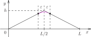
Figure 2: Illustration of the original initial condition for the position of the plucked string, superposed with the filtered initial condition.

One can change this by applying the first-order linear low-lass filter to the initial condition, with a range parameter $\varepsilon$, which has the effect of exchanging the top of the triangle for an inverted arc of parabola that fits the two remaining segments in such a way that the resulting function is continuous and differentiable, as shown in Figure 2. Since the coefficients of the equation do not depend on $x$, we may obtain the filtered solution by simply plugging the filter factor $[\sin(\pi k\varepsilon/L)/(\pi k\varepsilon/L)]$ into the series, thus obtaining at once the filtered solution,

$$f_{\varepsilon}(x,t) = \frac{8hL}{\pi^{3}\varepsilon}\sum_{j=0}^{\infty}\frac{(-1)^{j}}{k^{3}}\,\sin\!\left(\pi\frac{k\varepsilon}{L}\right)\cos\!\left(\pi\frac{k\nu t}{L}\right)\sin\!\left(\pi\frac{kx}{L}\right),$$

$$\frac{\partial f_{\varepsilon}(x,t)}{\partial t} = -\,\frac{8h\nu}{\pi^{2}\varepsilon}\sum_{j=0}^{\infty}\frac{(-1)^{j}}{k^{2}}\,\sin\!\left(\pi\frac{k\varepsilon}{L}\right)\sin\!\left(\pi\frac{k\nu t}{L}\right)\sin\!\left(\pi\frac{kx}{L}\right),$$

$$\frac{\partial^{2}f_{\varepsilon}(x,t)}{\partial t^{2}} = -\,\frac{8h\nu^{2}}{L\pi\varepsilon}\sum_{j=0}^{\infty}\frac{(-1)^{j}}{k}\,\sin\!\left(\pi\frac{k\varepsilon}{L}\right)\cos\!\left(\pi\frac{k\nu t}{L}\right)\sin\!\left(\pi\frac{kx}{L}\right).$$

We see that now the series for the position and for the velocity are both absolutely and uniformly convergent. The series for the acceleration is now convergent, although it is still not absolutely or uniformly convergent. It now represents two rectangular pulses of width $\varepsilon$ propagating back and forth along the string and reflecting at its ends, with inversion of their sign. This means that each point of the string is now subjected repeatedly to a large but finite acceleration, proportional to $1/\varepsilon$, acting for a very short time, of the order of $\varepsilon/\nu$. One can show that the series for the acceleration is convergent using trigonometric identities to write it in the form

$$\frac{\partial^{2}f_{\varepsilon}(x,t)}{\partial t^{2}} = -\,\frac{h\nu^{2}}{L\pi\varepsilon}\sum_{j=0}^{\infty}\frac{1}{k}\,\left[\rule{0.0pt}{25.83325pt}\hskip 6.99997pt\sin\!\left(k\pi\frac{L+\varepsilon-\nu t-x}{L}\right)+\sin\!\left(k\pi\frac{L-\varepsilon+\nu t+x}{L}\right)\right.+$$

$$\left.\rule{0.0pt}{12.91663pt}\hskip 60.00009pt-\sin\!\left(k\pi\frac{L+\varepsilon+\nu t+x}{L}\right)-\sin\!\left(k\pi\frac{L-\varepsilon-\nu t-x}{L}\right)\right.+$$

$$\left.\rule{0.0pt}{25.83325pt}\hskip 60.00009pt-\sin\!\left(k\pi\frac{L+\varepsilon-\nu t+x}{L}\right)-\sin\!\left(k\pi\frac{L-\varepsilon+\nu t-x}{L}\right)\right.+$$

$$\left.\rule{0.0pt}{25.83325pt}\hskip 60.00009pt+\sin\!\left(k\pi\frac{L+\varepsilon+\nu t-x}{L}\right)+\sin\!\left(k\pi\frac{L-\varepsilon-\nu t+x}{L}\right)\hskip 10.00002pt\right].$$

These eight sine series have coefficients that converge monotonically to zero and therefore are convergent by the Dirichlet test, or alternatively by the monotonicity criterion discussed in [3]. Therefore, the series for the acceleration is in fact convergent after the application of the filter. Note that these eight series represent travelling waves propagating on an infinite string of which our vibrating string can be thought of as a given segment.

We can say that the application of the filter in fact improved the representation of the physical system in this problem, because it is unreasonable to imagine that a real physical string could have the initial format used at first, with the point of non-differentiability. For one thing, it would be necessary to use some physical object such as a nail or peg to hold it in its initial position prior to release. The radius of this object is an excellent candidate for $\varepsilon$. In any case, one cannot hope to make a perfect angle by bending a material string that has a finite and non-zero thickness. The radius of the cross-section of the string would be another excellent candidate for $\varepsilon$. In this way we see that the application of the filter brought the representation of the physical system closer to reality.

B.2 Potential in a Rectangular Box

Consider an empty two-dimensional rectangular box with electrically conducting walls kept at given values of the electric potential, as shown on Figure 3. The electrostatic potential within the box is given by Laplace’s equation,

$$\frac{\partial^{2}}{\partial x^{2}}\phi(x,y)+\frac{\partial^{2}}{\partial y^{2}}\phi(x,y)=0.$$

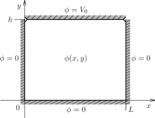
Figure 3: The two-dimensional rectangular box and the boundary values for the electric potential.

The boundary values are as shown in the illustration. Note that, as indicated in the figure, the top surface cannot be considered as being in electric contact with the other ones, if the potentials are to be kept as shown. However, in the resolution of the problem this fact is not taken explicitly into account. The solution of the problem can be given in terms of mixed Fourier and hyperbolic series for the electric potential and for the two Cartesian components of the electric field, which is obtained as minus the gradient of the potential,

$$\phi(x,y) = \frac{4V_{0}}{\pi}\sum_{j=0}^{\infty}\frac{1}{k}\,\sin\!\left(\pi\frac{kx}{L}\right)\,\frac{\sinh\!\left(\pi{\displaystyle\frac{\displaystyle ky}{\displaystyle L}}\right)}{\sinh\!\left(\pi{\displaystyle\frac{\displaystyle kh}{\displaystyle L}}\right)},$$

$$E_{x}(x,y) = -\,\frac{4V_{0}}{L}\displaystyle\sum_{j=0}^{\infty}\cos\!\left(\pi\frac{kx}{L}\right)\,\frac{\sinh\!\left(\pi{\displaystyle\frac{\displaystyle ky}{\displaystyle L}}\right)}{\sinh\!\left(\pi{\displaystyle\frac{\displaystyle kh}{\displaystyle L}}\right)},$$

$$E_{y}(x,y) = -\,\frac{4V_{0}}{L}\displaystyle\sum_{j=0}^{\infty}\sin\!\left(\pi\frac{kx}{L}\right)\,\frac{\cosh\!\left(\pi{\displaystyle\frac{\displaystyle ky}{\displaystyle L}}\right)}{\sinh\!\left(\pi{\displaystyle\frac{\displaystyle kh}{\displaystyle L}}\right)},$$

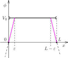
Figure 4: The original boundary condition on the top surface of the box, superposed with the filtered boundary condition.

where $k=2j+1$. Note that so long as $y<h$ all these series are absolutely convergent and uniformly convergent along the direction $x$. In fact, in this case they converge to $C^{\infty}$ functions of $x$. This is so because the ratios of hyperbolic functions decrease to zero exponentially fast with $k$ when $y<h$. However, for $y=h$, that is at the top surface, these factors cease to approach zero as $k\to\infty$, and then the convergence status is much more precarious. The series for the potential is still convergent, but not absolute or uniformly so. The series for the field components diverge everywhere. This is caused by the neglect to take into account the fact that the top surface must be electrically isolated from the others, which causes the appearance of infinite electric fields near the two top corners of the box. This is expressed as a singular boundary condition at the top surface, with the form of a rectangular pulse, discontinuous at $x=0$ and $x=L$, as shown in Figure 4.

One can change this by applying the first-order linear low-lass filter to the boundary condition at the top surface, with a small range parameter $\varepsilon$, which has the effect of exchanging the discontinuities for two very steep potential ramps, as is also shown in Figure 4. Since the coefficients of the differential equation do not depend on $x$, we may at once write the solution for the filtered potential and for the filtered electric field components, by simply plugging the filter factor $[\sin(\pi k\varepsilon/L)/(\pi k\varepsilon/L)]$ into the series,

$$\phi_{\varepsilon}(x,y) = \frac{4V_{0}L}{\pi^{2}\varepsilon}\sum_{j=0}^{\infty}\frac{1}{k^{2}}\,\sin\!\left(\pi\frac{k\varepsilon}{L}\right)\sin\!\left(\pi\frac{kx}{L}\right)\,\frac{\sinh\!\left(\pi{\displaystyle\frac{\displaystyle ky}{\displaystyle L}}\right)}{\sinh\!\left(\pi{\displaystyle\frac{\displaystyle kh}{\displaystyle L}}\right)}.$$

$$E_{\varepsilon,x}(x,y) = -\,\frac{4V_{0}}{\pi\varepsilon}\sum_{j=0}^{\infty}\frac{1}{k}\,\sin\!\left(\pi\frac{k\varepsilon}{L}\right)\cos\!\left(\pi\frac{kx}{L}\right)\,\frac{\sinh\!\left(\pi{\displaystyle\frac{\displaystyle ky}{\displaystyle L}}\right)}{\sinh\!\left(\pi{\displaystyle\frac{\displaystyle kh}{\displaystyle L}}\right)},$$

$$E_{\varepsilon,y}(x,y) = -\,\frac{4V_{0}}{\pi\varepsilon}\sum_{j=0}^{\infty}\frac{1}{k}\,\sin\!\left(\pi\frac{k\varepsilon}{L}\right)\sin\!\left(\pi\frac{kx}{L}\right)\,\frac{\cosh\!\left(\pi{\displaystyle\frac{\displaystyle ky}{\displaystyle L}}\right)}{\sinh\!\left(\pi{\displaystyle\frac{\displaystyle kh}{\displaystyle L}}\right)}.$$

The series for the potential is now absolutely and uniformly convergent everywhere within the box, including the top surface. The series for the field components are still strongly convergent to $C^{\infty}$ functions away from the top surface, and at that surface they are convergent almost everywhere, although not absolutely or uniformly so. The solution changes significantly only in the neighborhood of the two points were the original singularity on the boundary conditions was located. If we write, as an example, the field component $E_{\varepsilon,x}(x,y)$ at the top surface, we get

$$E_{\varepsilon,x}(x,h)=-\,\frac{4V_{0}}{\pi\varepsilon}\sum_{j=0}^{\infty}\frac{1}{k}\,\sin\!\left(\pi\frac{k\varepsilon}{L}\right)\cos\!\left(\pi\frac{kx}{L}\right),$$

where $k=2j+1$. One can show that this series is everywhere convergent using trigonometric identities to write it in the form

$$E_{\varepsilon,x}(x,h)=\frac{2V_{0}}{\pi\varepsilon}\sum_{j=0}^{\infty}\frac{1}{k}\,\left[\sin\!\left(\pi k\frac{x-\varepsilon}{L}\right)-\sin\!\left(\pi k\frac{x+\varepsilon}{L}\right)\right].$$

The two sine series obtained in this way have coefficients that converge monotonically to zero and therefore are convergent by the Dirichlet test, or alternatively by the monotonicity criterion discussed in [3]. Therefore, the series for $E_{\varepsilon,x}(x,y)$ is in fact everywhere convergent after the application of the filter. The other field component at the top surface can be analyzed in a similar way. It is given by

$$E_{\varepsilon,y}(x,h)=-\,\frac{4V_{0}}{\pi\varepsilon}\sum_{j=0}^{\infty}\frac{1}{k}\,\sin\!\left(\pi\frac{k\varepsilon}{L}\right)\sin\!\left(\pi\frac{kx}{L}\right)\,\frac{\cosh\!\left(\pi{\displaystyle\frac{\displaystyle kh}{\displaystyle L}}\right)}{\sinh\!\left(\pi{\displaystyle\frac{\displaystyle kh}{\displaystyle L}}\right)}.$$

For large values of $k$ the ratio of hyperbolic functions tends to $1$. In this case the analysis with the monotonicity criterion shown that the series is convergent at all points except two, the points $x=\varepsilon$ and $x=L-\varepsilon$. Further application of the first-order filter, or the application of the second-order filter, can then be used to further improve the situation.

We can say that the introduction of the filter in fact improved the representation of the physical system in this problem, from the physical standpoint, because the two steep potential ramps can be understood as a representation of the electric potential within two thin slices of an insulating material, of thickness $\varepsilon$, inserted between the top surface and the two lateral ones. In fact, within a good dielectric this is a very good representation of the electric potential. Once more we see that the introduction of the filter brought the description of the physical system closer to reality.

The two remaining isolated points of divergence are in the field component normal to the surface, exactly at the point where we have the material interfaces between the conducting material of the upper wall and the insulating dielectric of the thin slices. This suggests that these remaining divergences are related to the imperfect representation of these material interfaces. In fact, the inclusion of the thin insulating slices introduces into the system two electric capacitors, and the divergences may be related to the known edge effects that occur at the edges of the plates of any capacitor, where electric charges tend to accumulate.

In this case the physical scale involved is that of the inter-material transition at the interface, which may go right down to the molecular level. Therefore it seems appropriate to use once more the first-order filter on the boundary condition, this time with a range parameter $\varepsilon^{\prime}\ll\varepsilon$. This will have the effect of smoothing out the sharp transitions between the two materials. Regardless of the value of the parameter $\varepsilon^{\prime}$, this will render all the series absolutely and uniformly convergent everywhere, since they will then all have at least a factor of $1/k^{2}$ in their coefficients.

The actual values of the field near the material interfaces will of course depend on $\varepsilon^{\prime}$. If it turns out to be possible to measure these field values well enough, it may be possible to determine an optimal value of $\varepsilon^{\prime}$ based on experimental data, which will then establish a rough model for the description of the material interface, from the macroscopic point of view. We see therefore that this mathematical technique may be turned into a tool for probing into aspects of the structure of the physical world.

B.3 Heat Conduction in a Cylinder

Consider the two-dimensional cross-section of an infinite solid cylinder made of a heat-conducting material. Suppose that its two sides are in contact with heat baths, one above and one below, as shown in Figure 5. The system reaches a state of stationary heat conduction given by Laplace equation in cylindrical coordinates for the temperature $u(r,\theta)$,

$$r\,\frac{\partial}{\partial r}\left[r\,\frac{\partial}{\partial r}u(r,\theta)\right]+\frac{\partial^{2}}{\partial\theta^{2}}u(r,\theta)=0.$$

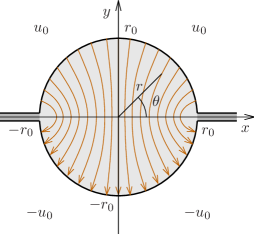
Figure 5: The infinite cylinder and the boundary conditions for the temperature.

The two boundary values are shown in the illustration. In the standard (and simpler) formulation of the problem, one considers that the two heat baths are thermally isolated from each other, but the thermally isolating material needed to accomplish this is not taken into account explicitly. The solution of the problem can be given in terms of mixed power and Fourier series for the static temperature and for the radial and angular components of the heat flux density, which is related to the gradient of the temperature,

$$u(r,\theta) = \frac{4u_{0}}{\pi}\sum_{j=0}^{\infty}\frac{1}{k}\left(\frac{r}{r_{0}}\right)^{k}\sin(k\theta),$$

$$\jmath_{r}(r,\theta) = -\,\frac{4c\mu\kappa u_{0}}{\pi r_{0}}\sum_{j=0}^{\infty}\left(\frac{r}{r_{0}}\right)^{k-1}\sin(k\theta),$$

$$\jmath_{\theta}(r,\theta) = -\,\frac{4c\mu\kappa u_{0}}{\pi r_{0}}\sum_{j=0}^{\infty}\left(\frac{r}{r_{0}}\right)^{k-1}\cos(k\theta),$$

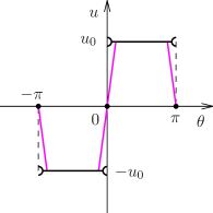
Figure 6: The original boundary conditions superposed with the filtered boundary conditions.

where $k=2j+1$ and the constants appearing in $\jmath_{r}(r,\theta)$ and $\jmath_{\theta}(r,\theta)$ characterize the material. Note that so long as $r<r_{0}$ all the series are strongly convergent to $C^{\infty}$ functions, due to the exponential decay with $k$ of the factors involving the ratio $(r/r_{0})$. However, at the surface of the cylinder, for $r=r_{0}$, the series for the temperature is not absolutely or uniformly convergent, but only point-wise convergent. Besides, at this surface the series for the components of the heat flux density are simply everywhere divergent. This is caused by the neglect to take into account the necessity to have a layer of isolating material of finite thickness between the two heat baths, which causes the presence of infinite heat fluxes at the points where these two heat baths are infinitely close to each other, and connected to each other through the material of the cylinder.

One can change this by applying the first-order linear low-pass filter to the boundary condition at the surface of the cylinder, with a small angular range parameter $\epsilon$. This exchanges the two discontinuities of the boundary temperature for two thin layers with steep variation of the temperature, as shown in Figure 6. Since the coefficients of the differential equation do not depend on $\theta$, we may write at once the filtered solution, by simply plugging the filter factor $[\sin(k\epsilon)/(k\epsilon)]$ into the series,

$$u_{\epsilon}(r,\theta) = \frac{4u_{0}}{\pi\epsilon}\sum_{j=0}^{\infty}\frac{\sin(k\epsilon)}{k^{2}}\left(\frac{r}{r_{0}}\right)^{k}\sin(k\theta),$$

$$\jmath_{\epsilon,r}(r,\theta) = -\,\frac{4c\mu\kappa u_{0}}{\pi r_{0}\epsilon}\sum_{j=0}^{\infty}\frac{\sin(k\epsilon)}{k}\left(\frac{r}{r_{0}}\right)^{k-1}\sin(k\theta),$$

$$\jmath_{\epsilon,\theta}(r,\theta) = -\,\frac{4c\mu\kappa u_{0}}{\pi r_{0}\epsilon}\sum_{j=0}^{\infty}\frac{\sin(k\epsilon)}{k}\left(\frac{r}{r_{0}}\right)^{k-1}\cos(k\theta),$$

where $k=2j+1$. The series for the temperature is now absolutely and uniformly convergent everywhere, and the series for the components of the heat flux density are point-wise convergent almost everywhere at the surface of the cylinder. If we write for example the components $\jmath_{\epsilon,\theta}(r,\theta)$ at the surface, we get

$$\jmath_{\epsilon,\theta}(r_{0},\theta)=-\,\frac{4c\mu\kappa u_{0}}{\pi r_{0}\epsilon}\sum_{j=0}^{\infty}\frac{1}{k}\,\sin(k\epsilon)\cos(k\theta).$$

One can show that this series is convergent everywhere using trigonometric identities to write it in the form

$$\jmath_{\epsilon,\theta}(r_{0},\theta)=\frac{2c\mu\kappa u_{0}}{\pi r_{0}\epsilon}\sum_{j=0}^{\infty}\frac{1}{k}\,\left\{\rule{0.0pt}{10.76385pt}\sin[k(\theta-\epsilon)]-\sin[k(\theta+\epsilon)]\right\}.$$

The two sine series obtained in this way have coefficients that converge monotonically to zero and therefore are convergent by the Dirichlet test, or alternatively by the monotonicity criterion discussed in [3]. The other field component at the surface can be analyzed in a similar way. It is given by

$$\jmath_{\epsilon,r}(r_{0},\theta)=-\,\frac{4c\mu\kappa u_{0}}{\pi r_{0}\epsilon}\sum_{j=0}^{\infty}\frac{1}{k}\,\sin(k\epsilon)\sin(k\theta).$$

In this case the analysis with the monotonicity criterion shown that the series is convergent at all points except four, the points $\theta=\pm\epsilon$, $\theta=\pi-\epsilon$ and $\theta=-\pi+\epsilon$. Further application of the first-order filter, or the application of the second-order filter, can then be used to further improve the situation.

We can say that the introduction of the filter in fact improved the representation of the physical system in this problem, from the physical standpoint, because the two steep variations of the temperature can be understood as representations of the temperature within two thin slices of a thermally insulating material, of angular thickness $2\epsilon$, inserted between the two heath baths. Once again we see that the introduction of the filter brought the description of the physical system closer to reality.

Just an in the previous example, the remaining points of divergence are in the component of the heat flux density normal to the surface, exactly at the point where we have the material interfaces between the heat baths and the thermally insulating material of the thin slices. This once more suggests that these remaining divergences are related to the imperfect representation of these material interfaces. Therefore it seems appropriate to use once more the first-order filter on the boundary condition, with a range parameter $\epsilon^{\prime}\ll\epsilon$ which could go all the way down to the molecular scale.

Although a direct and detailed physical interpretation seems not to be immediately apparent in this case, essentially the same comments made in the last example about the role of a second application of the filter are also true in this case. Clearly it will have the effect of smoothing out the sharp transitions between the two materials. Regardless of the value of the parameter $\epsilon^{\prime}$, it will certainly render all the series absolutely and uniformly convergent everywhere, since they will then all have at least a factor of $1/k^{2}$ in their coefficients.

Note that since the derivation of the heat equation from fundamental physical principles has a statistical character, involving averages over large numbers of molecules of the material involved, it is not unreasonable that one may meet with difficulties in its description of nature when one goes down to the molecular scale, as we have done here. We may interpret these isolated singularities as consequences of the use of a physical theory at the very edge of its recognized domain of validity.

References

- [1] See, for example, R. V. Churchill and J. W. Brown, “Fourier Series and Boundary Value Problems”, McGraw-Hill Book Co., 2011, and the references therein.
- [2] J. L. deLyra, “Fourier Theory on the Complex Plane I – Conjugate Pairs of Fourier Series and Inner Analytic Functions”, arXiv: 1409.2582.
- [3] J. L. deLyra, “Fourier Theory on the Complex Plane II – Weak Convergence, Classification and Factorization of Singularities”, arXiv: 1409.4435.
-
[4]
A compressed tar file containing the program used to
plot the graphs of the kernels, and some associated utilities, can be
found at the URL
http://latt.if.usp.br/scientific-pages/lpffsapde/