Synchronizing spatio-temporal chaos with imperfect models: a stochastic surface growth picture

Abstract

We study the synchronization of two spatially extended dynamical systems where the models have imperfections. We show that the synchronization error across space can be visualized as a rough surface governed by the Kardar-Parisi-Zhang equation with both upper and lower bounding walls corresponding to nonlinearities and model discrepancies, respectively. Two types of model imperfections are considered: parameter mismatch and unresolved fast scales, finding in both cases the same qualitative results. The consistency between different setups and systems indicates the results are generic for a wide family of spatially extended systems.

Identical chaotic systems are able to perfectly synchronize when coupled. This phenomenon is very attractive from a theoretical perspective and has a tremendous potential for technological applications, like for instance, secure optical communications. Chaotic synchronization of spatially extended dynamical systems plays also a fundamental role in forecasting applications and observation data assimilation in geoscience. Unfortunately, dynamical systems are far from identical in practical applications and synchronization of high dimensional systems in the real world becomes severely hampered by imperfections like parameter mismatches and unresolved scales. Understanding the bounds to synchronization for imperfect systems, the effect of finite non-small parameter deviations, and limited resolution on the statistics of the synchronization error is essential for real applications. The theoretical challenge is to describe synchronization of imperfect models under the umbrella of a generic stochastic theory that describes the most outstanding features in a model–independent fashion.

I Introduction

Synchronization phenomena between two identical chaotic systems have been exhaustively investigated since the 1990s Pecora et al. (1997); Pikovsky et al. (2001); Boccaletti et al. (2002). It was soon realized that unavoidable differences between two interacting systems $\mathbf{u}$ and $\mathbf{v}$ makes generically impossible to observe complete synchronization, i.e. $\mathbf{w}(t)\equiv\mathbf{v}(t)-\mathbf{u}(t)=0$, in real systems. This led to the concept of ‘attractor bubbling’ Ashwin et al. (1994), which is successfully explained in terms of certain unstable periodic orbits Heagy et al. (1995); Venkataramani et al. (1996). However, in many practical situations the systems under investigation are spatially extended (or high-dimensional) and strongly chaotic, rendering that theoretical framework clearly inadequate. A prominent example of the latter is the coupling of lasers with optical feedback, customarily used in encrypted communications. The problem of synchronization of two spatially extended nonidentical dynamical systems has been considered before Boccaletti et al. (1999); Duane and Tribbia (2001); Ginelli et al. (2009) (see also Revuelta et al. (2002); Cohen et al. (2008); Huang et al. (2009) for examples of time-delayed systems). Most of these previous works made essentially phenomenological explorations, except for the theoretical work of Ginelli et al. Ginelli et al. (2009) where a certain scaling relation was found for an infinitesimal parameter mismatch.

The purpose of the present study is to provide a qualitative picture of partial synchronization of spatially extended nonidentical systems for finite non-small parameter mismatch and/or significant model imperfections. Our aim is to obtain a stochastic field-theoretical description of synchronization for dynamical systems with significant dissimilarities and explore to what extent this field theory is valid for different types of model discrepancies. Such a theoretical description will enhance our understanding on how partial synchronization is achieved, to what degree, and what are the limiting factors to synchronize nonidentical systems in real-world applications.

Our approach builds upon the seminal work of Ahlers and Pikovsky Ahlers and Pikovsky (2002) that made a connection between the synchronization error of two coupled identical spatially extended systems and the dynamics of rough surfaces described by the ‘bounded Kardar-Parisi-Zhang’ (bKPZ) equation Tu et al. (1997). Interestingly, the bKPZ class also characterizes the synchronization error between two (identical) time-delayed systems Szendro and López (2005). In the presence of dissimilarities of the models, our framework permits to qualitatively understand the dependence of the synchronization error statistics on the coupling strength.

Although not crucial for our main conclusions, in this work we consider a master-slave (also called drive-response or emitter-receiver) configuration where system $\mathbf{u}$ (the master) forces $\mathbf{v}$ (the slave). This synchronization setup, so-called unidirectional coupling, is used, for instance, in encrypted communications with chaos VanWiggeren and Roy (1998); Argyris et al. (2005). Remarkably, unidirectional coupling is also relevant in certain data assimilation techniques that are widely used in geoscience. Indeed, the technique termed nudging Hoke and Anthes (1976) is a classical data-assimilation method in which the unavoidably imperfect model is coupled to the ‘truth’ or ‘reality’ using (imperfect and sparse) observations. By means of unidirectional coupling the model “assimilates” the reality, and the model’s variables serve as an estimator of the state of the truth (say the atmosphere or the ocean) from observations Kalnay (2002). Unsurprisingly, the relationship between synchronization and ‘nudging’ has been highlighted and studied in the past Yang et al. (2006); Duane et al. (2006); Szendro et al. (2009a); Abarbanel et al. (2010).

The paper is organized as follows. In Sec. II we present the models we have used in our numerical simulations, and in Sec. III we review the relation between the bKPZ equation and complete synchronization of spatio-temporal chaos. In Secs. IV and V we present our numerical results for two typical situations: the case of a slave with significant parameter mismatch with respect to the master and, on the other hand, a situation where the slave is lacking the variables corresponding to the small length scale dynamics. The latter is specially relevant in some data assimilation applications in geoscience, where the models that are “coupled” to reality only describe the atmosphere or ocean state above a certain scale Yang et al. (2006); Duane et al. (2006); Szendro et al. (2009a); Abarbanel et al. (2010). Finally, in Sec. VI we interpret our results by the light of a surface picture of the synchronization error dynamics and summarize them.

II Models

Let us first start summarizing the type of master-slave configurations we will consider in this paper. Typically, our results will apply to systems that fulfill the following properties:

• The master and the slave are spatially extended systems with spatio-temporally chaotic dynamics. They can be either continuous or discrete in both space and time.

• The systems are assumed to be extended in one lateral spatial dimension (though not fundamental differences should arise in larger dimensions). Note that time-delayed systems belong to this category in virtue of a coordinate transformation, see Sec. II.1.3.

• The equations governing the master and the (uncoupled) slave systems are nonidentical, due to either a parameter mismatch or the existence of unresolved degrees of freedom.

• The coupling between both systems is dense (ideally at all points). Note that, from an experimental point of view, this is more easily achieved for coupled time-delayed systems than for real spatially extended systems. Actually, the premise of a dense constant coupling is generally assumed in any study of identical systems synchronization that we are aware of.

The system sizes we use in our simulations are large enough to allow the systems to exhibit spatially extended chaos. As we shall see, the synchronization threshold is not a critical point in the case of nonsmall parameter mismatch and, therefore, there are not finite-size corrections to scaling to take care of or other subtleties associated with critical point phenomena. This allows us to obtain generic properties with relatively modest system sizes, as compared with those needed in studies of synchronization of identical systems at the critical point.

In the remainder of this section we introduce the models used in the numerical simulations presented in this paper.

II.1 Spatially-extended systems with parameter mismatch

II.1.1 Coupled-map lattice

Coupled-map lattices (CMLs) are particularly efficient for numerical simulations of spatio-temporal chaos. In a master-slave configuration we have

$$u(x,t+1)=(1+\varepsilon{\cal D})f_{m}(u(x,t)),$$ (1)

for the master, and

$$v(x,t+1) = (1+\varepsilon{\cal D})[\gamma f_{m}(u(x,t))+$$ (2)

$$+ (1-\gamma)f_{s}(v(x,t))],$$

for the slave. $\cal D$ is the discrete Laplacian:

$${\cal D}G(x)=G(x-1)-2G(x)+G(x+1),$$

and periodic boundary conditions are assumed in the spatial coordinate $x=1,\ldots,L$. We adopt the fixed value $\varepsilon=1/3$ for the diffusion coefficient. We vary the coupling parameter $\gamma$ that controls the input strength of the master on the slave. In this work we choose the system size to be $L=4096$, which is large enough to capture generic phenomena in extended systems. The local dynamics is chosen to obey the logistic map $f_{m,s}(z)=\mu_{m,s}-z^{2}$, with $\mu_{m}=1.9$ (for the master) and $\mu_{s}=\mu_{m}+\Delta\mu$ (for the slave) taking values corresponding to a chaotic parameter region of the map. We study the effect of a finite and non-small parameter mismatch $\Delta\mu$ on the synchronization error.

II.1.2 Lorenz-96 model

The Lorenz-96 model Lorenz (1996); Lorenz and Emanuel (1998) was originally introduced as a toy model of the atmosphere consisting of $L$ nodes each representing a scalar variable at one site on a latitude circle. The model is, moreover, consistent with a discretization of the damped Burgers-Hopf equation under forcing Majda and Wang (2006): $\partial_{t}u-u\partial_{x}u=-\gamma\,u+F$. Unidirectional coupling between two Lorenz-96 models yields the following system of ordinary differential equations:

$$\dot{u_{i}} = u_{i-1}\left(u_{i+1}-u_{i-2}\right)-u_{i}+F_{m}$$ (3)

$$\dot{v_{i}} = v_{i-1}\left(v_{i+1}-v_{i-2}\right)-v_{i}+F_{s}+\gamma(u_{i}-v_{i})$$ (4)

with $i=1,\ldots,L=1024$, and periodic boundary conditions: $u_{0}=u_{L}$, $u_{-1}=u_{L-1}$, and $u_{L+1}=u_{1}$. The external forcing is controlled by parameter $F_{m,s}$ and in the spirit of Lorenz formulation of the model it represents the input of energy coming from sun radiation. We chose $F_{m}=8$, and $F_{s}=F_{m}+\Delta F$ for the master and slave systems, respectively. (We have also considered a mismatch in the dissipative term finding no significant difference.) With this value of the external forcing (or larger) the system exhibits (extensive) spatio-temporal chaos Pazó et al. (2008); Karimi and Paul (2010). The numerical integration was carried out using a fourth-order Runge-Kutta algorithm with time step ${\mathrm{d}}t=0.01$. We study synchronization error as the parameter mismatch $\Delta F$ is varied.

II.1.3 Time-delay system

The third model we consider consists of two coupled time-delayed ordinary differential equations:

$$\dot{u} = -au+b_{m}R(u_{\tau})$$ (5)

$$\dot{v} = -av+b_{s}R(v_{\tau})+\gamma(u-v)$$ (6)

where $u_{\tau}\equiv u(t-\tau)$, likewise for $v$. Time-delay systems play a fundamental role in the majority of studies on synchronization between high-dimensional chaotic systems. After the change of variables Arecchi et al. (1992)

$$t=x+\vartheta\tau$$ (7)

the delay system transforms into a one-dimensional spatially extended system with the spatial coordinate $x\in[0,\tau)$, and evolving with a discrete temporal variable $\vartheta=0,1,\ldots$. The perturbation dynamics of time-delay systems, in the large “size” limit ($\tau\gg 1$), is in all respects equivalent to that of standard spatio-temporal chaotic systems Pikovsky and Politi (1998); Pazó and López (2010). As a typical example we studied the Mackey-Glass system Mackey and Glass (1977):

$$R(\rho)=\frac{\rho}{1+\rho^{10}}.$$

The model parameters are set to $a=1$, $b_{m}=2$, $b_{s}=b_{m}+\Delta b$. The chosen delay time $\tau=2000$ is large enough to make the system highly chaotic. Complete synchronization for identical systems, $b_{m}=b_{s}$, was shown Szendro and López (2005) to belong to the bKPZ class, as occurs for standard spatially extended chaotic systems. The numerical integration used was a third-order Adams-Bashforth-Moulton predictor-corrector method Press et al. (1992) with time step $dt=0.02$ t.u.

II.2 Spatially-extended system with unresolved scales

In Sec. V we shall consider the case of synchronization of an imperfect slave system that does not contain the variables corresponding to the small scale dynamics present in the master. This two-scale situation is typically found in meteorology, for instance, where the models necessarily do not incorporate small-scale turbulence present in the actual atmosphere. The two-scale version of the Lorenz-96 model Lorenz (1996) is customarily used to study this effect by supplementing Eq. (3) with a second ring of fast evolving variables $y$. The complete system writes:

$$\dot{u}_{i}=u_{i-1}(u_{i+1}-u_{i-2})-u_{i}+F-\frac{\eta\,c}{b}\sum_{j=1}^{J}y_{j,i}$$ (8a)

$$c^{-1}\dot{y}_{j,i}=b\,y_{j+1,i}(y_{j-1,i}-y_{j+2,i})-y_{j,i}+\frac{|\eta|}{b}u_{i},$$ (8b)

where $i=1,\dots,L=36$, $j=1,\dots,J=10$, and periodic boundary conditions are assumed: $u_{L+1}=u_{1}$, $u_{0}=u_{L}$, $u_{-1}=u_{L-1}$, and $y_{J+1,i}=y_{1,i+1}$, $y_{J+2,i}=y_{2,i+1}$, $y_{0,i}=y_{J,i-1}$. The constant $c=10$ makes the characteristic time scale of the $y$ variables to be 10 times shorter than for the $u$ variables. The constant $\eta$ controls the coupling between the two layers, while other constants are taken here as originally adopted by Lorenz: $b=F=10$. With respect to the original formulation of the model, we have replaced $\eta$ by $|\eta|$ in Eq. (8b) in order to consistently explore also negative values of $\eta$. For $\eta=0$ the fast scale becomes irrelevant and the system is fully described by Eq. (8a) alone.

We adopt Eq. (8) for the master, while the slave system (lacking the fast variables $y$) is governed by Eq. (4) with the same forcing constant $F=10$ and size $L=36$ than the master. The numerical simulations were carried out using a fourth-order Runge-Kutta algorithm with time step $dt=10^{-3}$.

III Short overview of complete synchronization of spatio-temporal chaos

In order to construct a stochastic field description of synchronization under finite imperfections, we build upon the existing picture for synchronization between identical systems with smooth equations. An interesting and far-reaching result Pikovsky and Kurths (1994); Pikovsky and Politi (1998); Pazó et al. (2008) is that, for spatially extended systems, the spatio-temporal scaling properties of infinitesimal perturbations $\delta u$ are generically captured by a linear stochastic equation:

$$\partial_{t}\delta u=\xi\delta u+\partial_{xx}\delta u$$ (9)

where $\xi(x,t)$ is a white noise. Under a Hopf-Cole transformation

$$h(x,t)=\ln|\delta u(x,t)|,$$ (10)

and assuming the Stratonovich interpretation for the noise, we get the Kardar-Parisi-Zhang (KPZ) equation Kardar et al. (1986),

$$\partial_{t}h=\xi+(\partial_{x}h)^{2}+\partial_{xx}h.$$ (11)

It has been clearly demonstrated by Pikovsky et al. Pikovsky and Kurths (1994); Pikovsky and Politi (1998) that the main Lyapunov vector obeys scaling laws in perfect agreement with the universality class defined by KPZ, see also Pazó and López Pazó and López (2010) for equivalent results for time-delayed systems.

Following the same approach, Ahlers and Pikovsky Ahlers and Pikovsky (2002) proposed the following stochastic field equation for the synchronization error $w(x,t)=v(x,t)-u(x,t)$ between identical systems:

$$\partial_{t}w=(\xi-\gamma)w+\partial_{xx}w-p|w|^{p+1}$$ (12)

($p=2$ was explicitly used by Ahlers and Pikovsky Ahlers and Pikovsky (2002)). This is basically the stochastic equation (9) supplemented with a nonlinear saturation term Tu et al. (1997). Equation (12) with $p>0$ defines the multiplicative-noise (MN) universality class Muñoz and Hwa (1998); Muñoz et al. (2003) (also denoted MN1 class for the sake of distinguishing it from the complementary MN2 class corresponding to $p<0$).

Let $\gamma_{c}$ be the synchronization threshold such that the system fails to synchronize for $\gamma<\gamma_{c}$, while complete synchronization ($w(x,t)=0$) is the asymptotic state of Eq. (12) for $\gamma>\gamma_{c}$. For smooth systems $\gamma_{c}$ is precisely the point at which the synchronized state undergoes a transition from linear unstable to linearly stable.

An interesting observation is that under a Hopf-Cole transformation, $h=\ln|w|$, Eq. (12) yields the so-called bounded Kardar-Parisi-Zhang Tu et al. (1997) (bKPZ) equation:

$$\partial_{t}h=\xi-\gamma+(\partial_{x}h)^{2}+\partial_{xx}h-pe^{ph}.$$ (13)

The growth-limiting $e^{ph}$ term is a bound (or ‘upper wall’) that prevents $h$ from going to infinity for $\gamma<\gamma_{c}$, while for $\gamma>\gamma_{c}$ one has $h\to-\infty$ as time evolves (i.e. the synchronization error vanishes). Fig. 1(a) sketches snapshots of the log-transformed error $h$ for different values of $\gamma$. An important side effect of the upper wall is the progressive reduction of the width of the “surface” $h$ as $\gamma$ decreases from $\gamma_{c}$.

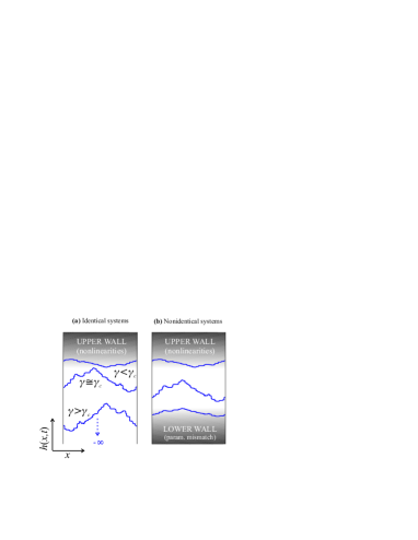
Figure 1: The curves sketch snapshots of $h(x,t)=\ln|w(x,t)|$ for different couplings $\gamma$. (a) Identical systems: Above threshold ($\gamma>\gamma_{c}$) the synchronization error drops to zero ($h\to-\infty$). As $\gamma$ decreases from $\gamma_{c}$, $\bar{h}(t)$ increases but the width of $h(x,t)$ decreases. (b) Non-identical systems: Parameter mismatches act as a lower wall that prevents the synchronization error from dropping to zero even for large $\gamma$ values. The maximum width of $h$ is roughly observed when $h$ is about equidistant from both upper and lower walls.

The bKPZ Eq. (13) was proposed Ahlers and Pikovsky (2002) as the minimal model of synchronization between extended systems, and this has been further confirmed by Szendro et al. Szendro et al. (2009b) and Ginelli et al. Ginelli et al. (2009), and Szendro and López Szendro and López (2005) for time-delay systems. Though a more complicated field equation could in principle occur Muñoz and Pastor-Satorras (2003), the bKPZ class (or its equivalent MN class) is quantitatively consistent with the numerical results.

Parameter mismatch between master and slave must have an effect that necessarily changes the picture presented in Fig. 1(a). Note that the absorbing state at $h=-\infty$ does not exist anymore, since complete synchronization, $w=0$, is no longer possible. The simplest way to implement the breakdown of the synchronized state is to introduce a new repulsive lower wall such that the error surface $h$ is kept away from $-\infty$, as sketched in Fig. 1(b). The joint effect of the upper and lower walls will be an error surface that lies somewhere in between. The mathematical form of the lower wall remains to be defined and will become clear after we discuss some numerical results. Suffices to say now that the lower wall is well described by a term proportional to the parameter mismatch, irrespective of the microscopic details of the model.

IV Numerical Results: Parameter mismatch

In this section we present the results of our simulations and give a rationale behind our proposed picture in Fig. 1(b) for non-identical systems. We postpone to Sec. VI deeper considerations about the results.

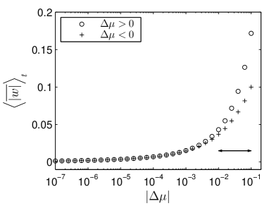
Figure 2: Average absolute-valued synchronization error at criticality $\gamma=0.289376\simeq\gamma_{c}$ for different values of $\Delta\mu$. The double sided arrow indicates the values, finite and non-infinitesimal, for the mismatch range considered in this paper.

IV.1 Coupled-map lattice

The error field $w(x,t)=v(x,t)-u(x,t)$ for coupled CMLs, see Eqs. (1) and (2), is governed by

$$w(x,t+1)=(1-\gamma)(1+\varepsilon{\cal D})\left[f_{s}(u(x,t)+w(x,t))-f_{m}(u(x,t))\right]$$ (14)

Inserting the explicit form of $f_{m,s}$ we obtain

$$w(x,t+1)=(1-\gamma)(1+\varepsilon{\cal D})\left[\Delta\mu-2u(x,t)w(x,t)-w(x,t)^{2}\right]$$ (15)

where $\Delta\mu=\mu_{s}-\mu_{m}$ is the parameter mismatch. For $\Delta\mu=0$ the synchronization threshold is at $\gamma_{c}\simeq 0.289376$. In Fig. 2 we may see that as $|\Delta\mu|$ increases the space-averaged absolute synchronization error

$$\overline{|w|}(t)=\frac{1}{L}\sum_{i=1}^{L}|w(x,t)|$$ (16)

grows accordingly. It is worth to stress here that parameter mismatch values considered in this work correspond to the region marked by a double-headed arrow in Fig. 2, these values are large and away from critical scaling region $|\Delta\mu|\to 0$. Also note the different curves for positive and negative $\Delta\mu$.

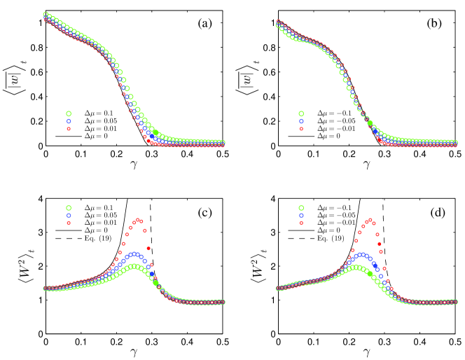
Figure 3: Coupled CMLs in Eqs. (1) and (2): (a,b) Average absolute error as a function of $\gamma$ for different values of $\Delta\mu$. (c,d) Time-averaged $W^{2}$ as a function of $\gamma$. Solid and dashed lines are obtained from Eqs. (18) and (19), respectively. Filled symbols signal the points corresponding to the threshold of generalized synchronization, $\gamma=\gamma_{g}$.

In Fig. 3(a,b) we plot the results of computing the temporal average of the space-averaged error $\left<\overline{|w|}\right>_{t}$ for different values of the mismatch $\Delta\mu$. For $\Delta\mu=0$ (solid line) $|w|$ drops to zero at the complete-synchronization threshold $\gamma=\gamma_{c}$, while for $\Delta\mu\neq 0$ $\left<\overline{|w|}\right>_{t}$ decreases monotonically as $\gamma$ increases but remains finite.

The statistic $\left<\overline{|w|}\right>_{t}$ does not inform about the homogeneity (or Gaussianity) of the synchronization error across space. This is conveniently analyzed by measuring the width of the error surface $h=\ln|w|$, which is quantified by the variance Szendro et al. (2009b):

$$W^{2}=\frac{1}{L}\sum_{x=1}^{L}[h(x,t)-\bar{h}(t)]^{2}.$$ (17)

This statistic quantifies of how many orders of magnitude the error amplitude $|w|$ spans, i.e. the degree of error localization in space. Large values are associated with a strong localization of the error at certain sites Szendro et al. (2009b), and a non-Gaussian distribution of $|w|$ across space (“spatial intermittency”, so to speak). We may see in Figs. 3(c,d) that $\left<W^{2}\right>_{t}$ is non-monotonic and reaches its maximum value at intermediate values of $\gamma$.

Equation (15) has two nonlinear terms, which suggests that we may consider two limits:

1. Large $|w|$ (small $\gamma$): in this limit we can neglect the $\Delta\mu$ term recovering the equation

   $$w(x,t+1)=(1-\gamma)(1+\varepsilon{\cal D})\times$$

   $$\left[-2u(x,t)w(x,t)-w(x,t)^{2}\right]$$ (18)

   for identical systems, where $|w|$ is known to be described by the MN equation (12) or its variant the bKPZ equation (13), see also Fig. 1(a).

2. Small $|w|$ (large $\gamma$): in this limit we can neglect the quadratic term (and any other higher-order term if they in fact exist) to get

   $$w(x,t+1)=(1-\gamma)(1+\varepsilon{\cal D})\times$$

   $$\left[\Delta\mu-2u(x,t)w(x,t)\right].$$ (19)

   It is convenient to stress that —irrespective of the particular systems involved— the constant term $O(w^{0})$ is a pure contribution of the parameter mismatch. In some systems, the parameter mismatch might also yield small irrelevant corrections in the linear $O(w^{1})$ and/or higher-order terms $O(w^{2}),O(w^{3}),\ldots$.

In Fig. 3(c,d) the solid and dashed lines are obtained simulating Eqs. (18) and (19), respectively. The overall behavior of $h=\ln|w|$, is like a KPZ surface in the presence of two bounds or walls: an upper wall—already present for $\Delta\mu=0$—coming from quadratic (or higher-order) terms, and a lower wall introduced by the parameter mismatch. Figure 1(b) sketches this simple (non-rigorous) picture: if $\gamma<\gamma_{c}$ ($\gamma>\gamma_{c}$) the upper (lower) prevents the “surface” $h$ from diverging to $+\infty$ ($-\infty$). One may see that, irrespective of the sign of $\Delta\mu$, as $|\Delta\mu|$ decreases the point of maximal $\left<W^{2}\right>_{t}$ moves to larger values of $\gamma$. This is consistent with our interpretation of a lower wall that retreats to $-\infty$ as $|\Delta\mu|\to 0$. At $\gamma=0$ master and slave evolve independently and we obtain a value of $\left<W^{2}\right>_{t}$ consistent with the expectation for Gaussian distributed error: $\left<W^{2}\right>_{t}=\pi^{2}/8=1.2337\ldots$; For large $\gamma$ values the width becomes even smaller than this value due to the strong pushing against the (lower) wall represented by the dashed line in Fig. 3(c,d).

Generalized synchronization

For the sake of comparison, a filled symbol for each data set is shown in Figs. 3, 4, and 5. This point marks the onset of generalized synchronization (GS), observed for $\gamma>\gamma_{s}$, and determined by the ‘auxiliary system method’ Abarbanel et al. (1996). In this method an auxiliary system (also called replica), identical to the slave system, is evolved in parallel with the same forcing from the master, and the convergence of the slave and its replica defines the GS. Although more stringent definitions of GS exist Afraimovich et al. (1986); Rulkov et al. (1995); Kocarev and Parlitz (1996), the ‘auxiliary system method’ Pecora et al. (1997); Parlitz et al. (1997) is intrinsically interesting because it signals the collapse of an ensemble of slaves if such a setup were used (for instance in data assimilation applications). The auxiliary system criterion has been often used in previous works on GS of spatio-temporal chaos, which include an experimental realization with a liquid crystal spatial light modulator with optoelectronic feedback Rogers et al. (2004), a numerical integration of the complex Ginzburg-Landau equation Hramov et al. (2005), and a reaction-diffusion system with a minimal excitable dynamics Berg et al. (2011). There is also a good number of studies devoted to GS in time-delayed systems Boccaletti et al. (2000); Zhan et al. (2003); Senthilkumar and Lakshmanan (2007); Senthilkumar et al. (2008). The monotonic displacement of the GS threshold with the parameter mismatch, see Fig. 3, stems from the changing chaoticity of the slave as its $\mu_{s}$ parameter is varied. It is also interesting to note that the onset of GS evidences an important difference between the upper wall and the lower wall. Though both walls act similarly preventing the surface $h$ from reaching $\pm\infty$ while reducing the width, the lower wall –in opposition to the upper wall– does not induce differences between the states of the replicas.

IV.2 Lorenz-96 model

The results for the Lorenz-96 model, Eqs. (3) and (4), are shown in Fig. 4, and they are qualitatively identical to those obtained in Fig. 3 for the CML. The surface width for large $\gamma$ can again be obtained by neglecting higher order terms $O(w^{2})$ in the governing equations for the error; analogously to Eq. (19):

$$\dot{w_{i}}=\Delta F-(1+\gamma)w_{i}+w_{i-1}\left(u_{i+1}-u_{i-2}\right)+u_{i-1}\left(w_{i+1}-w_{i-2}\right)$$ (20)

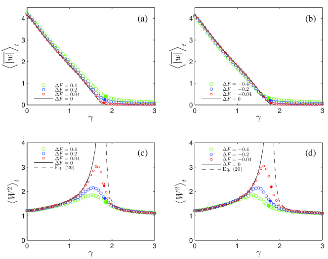
Figure 4: Coupled Lorenz-96 models in Eqs. (3) and (4): (a,b) Average absolute error as a function of $\gamma$ for different values of $\Delta F$. (c,d) Time-averaged $W^{2}$ as a function of $\gamma$. Filled symbols signal the points corresponding to the threshold of generalized synchronization, $\gamma=\gamma_{g}$.

IV.3 Time-delay system

The results for the time-delayed systems, Eqs. (5) and (6), are shown in Fig. 5. We have used the coordinate transformation (7) and studied the system like a spatially extended system of length $\tau$. As expected, we find no qualitative difference with respect to genuinely spatial systems. Note that, when going back to the original temporal framework, $\left<W^{2}\right>_{t}$ also serves to quantify the degree of intermittency (or non-Gaussianity) of the signal $w(t)=v(t)-u(t)$. In the small error approximation, neglecting higher order terms, we obtain:

$$\dot{w}=\Delta b\,R(u_{\tau})-(a+\gamma)w+b_{m}\,R^{\prime}(u_{\tau})\,w_{\tau}$$ (21)

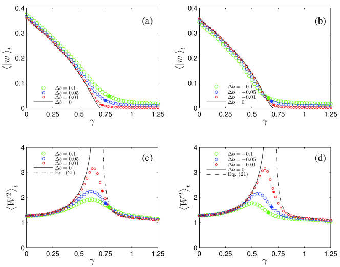
Figure 5: Coupled Mackey-Glass systems in Eqs. (5) and (6): (a,b) Average absolute error as a function of $\gamma$ for different values of $\Delta b$. (c,d) Time-averaged $W^{2}$ as a function of $\gamma$. Filled symbols signal the points corresponding to the threshold of generalized synchronization, $\gamma=\gamma_{g}$.

V Numerical Results: Unresolved scales

The question of the limits to synchronization of two systems in a master/slave configuration when the slave has a lower spatial resolution than the master is very relevant in practical applications, including forecasting and data assimilation in geoscience. The results with a two-scale Lorenz-96 model, Eq. (3) for the master and Eq. (8) as slave, are presented in Fig. 6. It is remarkable that the two systems are able to partially synchronize despite the obvious constitutive differences.

Interestingly, the statistical and dynamical properties of the synchronization error are qualitatively similar to those obtained in the case of parameter mismatch. Indeed, for very small $|\eta|$ one can see that the unresolved scales lead to an effective mismatch since the fast variables $y$ follow almost immediately the $u$ variable: $y_{j,i}\simeq\frac{|\eta|}{b}u_{i}$. Hence the $u$ variables of the master approximately obey the same one-scale equation than the slave but with a mismatch in the dissipative term:

$$\dot{u}_{i}=u_{i-1}\left(u_{i+1}-u_{i-2}\right)-\left(1+\frac{\eta|\eta|Jc}{b^{2}}\right)u_{i}+F\\$$ (22)

Coupling the slave system to this approximation of the master for $\eta=\pm 0.1$ we obtain the solid lines in Fig. 6, finding a very good agreement with results obtained using the original master system in Eq. (8).

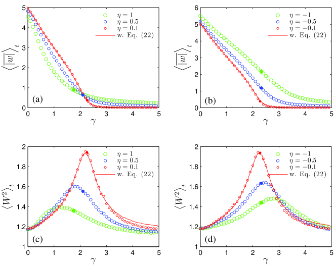
Figure 6: Two-scale Lorenz-96 model (master) coupled to a one-scale Lorenz-96 model (slave). (a,b) Average absolute error as a function of $\gamma$ for different values of $\eta$. (c,d) Time-averaged $W^{2}$ as a function of $\gamma$. In all panels the straight line is obtained when the master is replaced by an approximation given in Eq. (22) with $\eta=\pm 0.1$.

VI Discussion and Conclusions

All the numerical results presented so far can be understood as the combined effect of an upper and lower wall. In particular, the dependence of $W^{2}$ on $\gamma$ can be phenomenologically described by adding a term proportional to the mismatch $\Delta\mu$ to Eq. (12):

$$\partial_{t}w=\Delta\mu\,\zeta+(\xi-\gamma)w+\partial_{xx}w-p|w|^{p+1}$$ (23)

where $\zeta$ is a system-dependent (possibly fluctuating) term, whose detailed form does not affect the argument. Basically, the same equation was proposed by Ginelli et al. Ginelli et al. (2009) to describe the scaling behavior at $\gamma_{c}$ of $\left<\overline{|w|}\right>_{t}$ as $\Delta\mu\to 0$. In this paper we are well above the scaling regime but nevertheless Eq. (23) can be invoked to understand the basic features observed in Figs. 3, 4, 5, and 6. This complements the picture sketched in Fig. 1.

At small $\gamma$ the error $|w|$ is large and the mismatch term in Eq. (23) becomes negligible so that the curves $\left<W^{2}\right>_{t}$ converge for different values of the mismatch $\Delta\mu$, as observed in Figs. 3, 4, and 5. In contrast, for large $\gamma$ the error $|w|$ becomes small, so the $|w|^{p+1}$ term can be neglected and we are led, therefore, to the equation:

$$\partial_{t}w=\Delta\mu\,\zeta+(\xi-\gamma)w+\partial_{xx}w$$ (24)

We can divide the equation by $\Delta\mu$ and define the scaled variable $w^{\prime}=w/\Delta\mu$, which leads to the scaling relation

$$\left<\overline{|w|}\right>_{t}\propto|\Delta\mu|$$ (25)

in agreement with our simulations (not shown), and Eqs. (19)-(21). Moreover, note that Eq. (24) preserves the value of $W^{2}$ under changes of $\Delta\mu$ since it can be absorbed by a shift of the surface position $h^{\prime}=h-\ln\Delta\mu$. This explains the collapse of the curves $\left<W^{2}\right>_{t}$ at large $\gamma$ values for different intensities of the mismatch.

A final remark on the nature of the lower wall is in order. We may see that a straightforward application of the Hopf-Cole transformation to Eq. (24) yields a KPZ equation with an extra term of the form $\Delta\mu\,\zeta e^{-h}$, which is precisely a bKPZ equation with a lower-wall Muñoz and Hwa (1998). However, the exact correspondence with a bKPZ-type equation does not hold at least for two (not completely independent) reasons. Firstly, the function $\zeta$ is expected to be a fluctuating quantity in general, which is known Muñoz (2004) to have an important effect on assigning the corresponding universality class. Secondly, the absolute value $|w|$, which is implicit in the Hopf-Cole transformation, cannot be simply disregarded. In chaotic systems the sign of $w$ always fluctuates and the existence of zeros of $w$ is an unavoidable characteristic Szendro et al. (2007); Pazó et al. (2008). It turns out that these zeros do yield divergent contributions to the suggested (sign-independent) order parameter $\overline{|w|^{-1}}$ (see Al Hammal et al. Al Hammal et al. (2005) for further details on this rather technical question). We stress, nonetheless, that even if the lower wall is in mathematical terms an exponential bound with a fluctuating amplitude it has effectively the same qualitative effect as a simple exponential wall.

In this work we have put the focus on the nontrivial statistical features of the synchronization error between non-identical spatio-temporally chaotic systems. In the framework of a stochastic field theory that describes the synchronization error $w(x,t)$, the effect of the parameter mismatch is to give rise to a new lower wall (see Fig. 1), so that the absorbing state $w=0$ cannot be reached. The qualitative behavior of the ‘error surface’ $h=\ln|w|$ can be thus understood in terms of the competition between the two opposing walls: the standard upper wall that appears due to nonlinear saturation for large $|w|$, and the new lower wall associated with the model mismatch. The combined effect of the two walls permits the synchronization error to exhibit a significant deviation from Gaussianity only in a certain coupling range about the generalized synchronization threshold. Although our results have been obtained for systems with unidirectional coupling (master/slave configuration), they should apply equally well to the case of bidirectional coupling. The extension of our results to nonsmooth systems (generically associated with the directed percolation class Grassberger (1999); Ahlers and Pikovsky (2002); Szendro and López (2005); Ginelli et al. (2009)) remains as a task for future investigations.

We thank Alberto Carrassi for interesting discussions. DP acknowledges support by Cantabria International Campus, and by Ministerio de Economía y Competitividad (Spain) under the Ramón y Cajal programme.

References

- Abarbanel et al. (2010) Abarbanel, H. D. I., Kostuk, M., and Whartenby, W., “Data assimilation with regularized nonlinear instabilities,” Q. J. R. Meteorol. Soc. 136, 769–783 (2010).
- Abarbanel et al. (1996) Abarbanel, H. D. I., Rulkov, N. F., and Sushchik, M. M., “Generalized synchronization of chaos: The auxiliary system approach,” Phys. Rev. E 53, 4528–4535 (1996).
- Afraimovich et al. (1986) Afraimovich, V. S., Verichev, N. N., and Ravinovich, M. I., “Stochastic synchronization of oscillation in dissipative systems,” Radiophys. Quantum Electron. 29, 795–803 (1986).
- Ahlers and Pikovsky (2002) Ahlers, V. and Pikovsky, A., “Critical properties of the synchronization transition in space-time chaos,” Phys. Rev. Lett. 88, 254101 (2002).
- Al Hammal et al. (2005) Al Hammal, O., de los Santos, F., and Muñoz, M. A., “A non-order parameter Langevin equation for a bounded Kardar–Parisi–Zhang universality class,” J. Stat. Mech. 2005, P10013 (2005).
- Arecchi et al. (1992) Arecchi, F. T., Giacomelli, G., Lapucci, A., and Meucci, R., “Two-dimensional representation of a delayed dynamical system,” Phys. Rev. A 45, R4225 (1992).
- Argyris et al. (2005) Argyris, A., Syvridis, D., Larger, L., Annovazzi-Lodi, V., Colet, P., Fischer, I., García-Ojalvo, J., Mirasso, C. R., Pesquera, L., and Shore, K. A., “Chaos-based communications at high bit rates using commercial fibre-optic links,” Nature 438, 343–346 (2005).
- Ashwin et al. (1994) Ashwin, P., Buescu, J., and Stewart, I., “Bubbling of attractors and synchronisation of chaotic oscillators,” Phys. Lett. A 193, 126 – 139 (1994), ISSN 0375-9601.
- Berg et al. (2011) Berg, S., Luther, S., and Parlitz, U., “Synchronization based system identification of an extended excitable system,” Chaos 21, 033104 (2011).
- Boccaletti et al. (1999) Boccaletti, S., Bragard, J., Arecchi, F. T., and Mancini, H., “Synchronization in nonidentical extended systems,” Phys. Rev. Lett. 83, 536–539 (1999).
- Boccaletti et al. (2002) Boccaletti, S., Kurths, J., Osipov, G., Valladares, D.L., and Zhou, C.S., “The synchronization of chaotic systems,” Phys. Rep. 366, 1–101 (2002).
- Boccaletti et al. (2000) Boccaletti, S., Valladares, D. L., Kurths, J., Maza, D., and Mancini, H., “Synchronization of chaotic structurally nonequivalent systems,” Phys. Rev. E 61, 3712–3715 (2000).
- Cohen et al. (2008) Cohen, A. B., Ravoori, B., Murphy, T. E., and Roy, R., “Using synchronization for prediction of high-dimensional chaotic dynamics,” Phys. Rev. Lett. 101, 154102 (2008).
- Duane and Tribbia (2001) Duane, G. S. and Tribbia, J. J., “Synchronized chaos in geophysical fluid dynamics,” Phys. Rev. Lett. 86, 4298–4301 (2001).
- Duane et al. (2006) Duane, G. S., Tribbia, J. J., and Weiss, J. B., “Synchronicity in predictive modelling: a new view of data assimilation,” Nonlin. Proc. Geophys. 13, 601–612 (2006).
- Ginelli et al. (2009) Ginelli, F., Cencini, M., and Torcini, A., “Synchronization of spatio-temporal chaos as an absorbing phase transition: a study in 2+1 dimensions,” J. Stat. Mech. 2009, P12018 (2009).
- Grassberger (1999) Grassberger, P., “Synchronization of coupled systems with spatiotemporal chaos,” Phys. Rev. E 59, R2520 (1999).
- Heagy et al. (1995) Heagy, J. F., Carroll, T. L., and Pecora, L. M., “Desynchronization by periodic orbits,” Phys. Rev. E 52, R1253–R1256 (1995).
- Hoke and Anthes (1976) Hoke, J. E. and Anthes, R. A., “The initialization of numerical models by a dynamic-initialization technique,” Mon. Wea. Rev. 104, 1551–1556 (1976).
- Hramov et al. (2005) Hramov, A. E., Koronovskii, A. A., and Popov, P. V., “Generalized synchronization in coupled Ginzburg-Landau equations and mechanisms of its arising,” Phys. Rev. E 72, 037201 (2005).
- Huang et al. (2009) Huang, T., Li, C., Yu, W., and Chen, G., “Synchronization of delayed chaotic systems with parameter mismatches by using intermittent linear state feedback,” Nonlinearity 22, 569 (2009).
- Kalnay (2002) Kalnay, E., Atmospheric Modeling, Data Assimilation and Predictability (Cambridge University Press, Cambridge, 2002).
- Kardar et al. (1986) Kardar, M., Parisi, G., and Zhang, Y.-C., “Dynamic scaling of growing interfaces,” Phys. Rev. Lett. 56, 889–892 (1986).
- Karimi and Paul (2010) Karimi, A. and Paul, M. R., “Extensive chaos in the Lorenz-96 model,” Chaos 20, 043105 (2010).
- Kocarev and Parlitz (1996) Kocarev, L. and Parlitz, U., “Generalized synchronization, predictability, and equivalence of unidirectionally coupled dynamical systems,” Phys. Rev. Lett. 76, 1816–1819 (1996).
- Lorenz (1996) Lorenz, E. N., “Predictability - a problem partly solved,” in Proc. Seminar on Predictability Vol. I, edited by T. Palmer, ECMWF Seminar (ECMWF, Reading, UK, 1996) pp. 1–18.
- Lorenz and Emanuel (1998) Lorenz, E. N. and Emanuel, K. A., “Optimal sites for suplimentary weather observations: Simulations with a small model,” J. Atmos. Sci. 55, 399–414 (1998).
- Mackey and Glass (1977) Mackey, M. C. and Glass, L., “Oscillation and chaos in physiological control system,” Science 197, 287–289 (1977).
- Majda and Wang (2006) Majda, A. J. and Wang, X., Nonlinear Dynamics and Statistical Theories for Basic Geophyiscal Flows (Cambridge University Press, Cambridge, 2006).
- Muñoz (2004) Muñoz, M. A., “Advances in condensed matter physics,” (Nova Science Publishers, 2004) Chap. Multiplicative noise in non-equilibrium phase transitions: A tutorial, pp. 37–68.
- Muñoz et al. (2003) Muñoz, M. A., de los Santos, F., and Achahbar, A., “Critical behavior of a bounded Kardar-Parisi-Zhang equation,” Braz. J. Phys. 33, 443–449 (2003).
- Muñoz and Hwa (1998) Muñoz, M. A. and Hwa, T., “On nonlinear diffusion with multiplicative noise,” Europhys. Lett. 41, 147–152 (1998).
- Muñoz and Pastor-Satorras (2003) Muñoz, M. A. and Pastor-Satorras, R., “Stochastic theory of synchronization transitions in extended systems,” Phys. Rev. Lett. 90, 204101 (2003).
- Parlitz et al. (1997) Parlitz, U., Junge, L., and Kocarev, L., “Subharmonic entrainment of unstable period orbits and generalized synchronization,” Phys. Rev. Lett. 79, 3158–3161 (1997).
- Pazó and López (2010) Pazó, D. and López, J. M., “Characteristic Lyapunov vectors in chaotic time-delayed systems,” Phys. Rev. E 82, 056201 (2010).
- Pazó et al. (2008) Pazó, D., Szendro, I. G., López, J. M., and Rodríguez, M. A., “Structure of characteristic Lyapunov vectors in spatiotemporal chaos,” Phys. Rev. E 78, 016209 (2008).
- Pecora et al. (1997) Pecora, L. M., Carroll, T. L., Johnson, G. A., Mar, D. J., and Heagy, J. F., “Fundamentals of synchronization in chaotic systems, concepts, and applications,” Chaos 7, 520–543 (1997).
- Pikovsky and Politi (1998) Pikovsky, A. and Politi, A., “Dynamic localization of Lyapunov vectors in spacetime chaos,” Nonlinearity 11, 1049–1062 (1998).
- Pikovsky and Kurths (1994) Pikovsky, A. S. and Kurths, J., “Roughening interfaces in the dynamics of perturbations of spatiotemporal chaos,” Phys. Rev. E 49, 898–901 (1994).
- Pikovsky et al. (2001) Pikovsky, A. S., Rosenblum, M. G., and Kurths, J., Synchronization, a Universal Concept in Nonlinear Sciences (Cambridge University Press, Cambridge, 2001).
- Press et al. (1992) Press, W. H., Teukolsky, S. A., Vetterling, W. T., and Flannery, B. P., Numerical Recipes in Fortran 77: The Art of Scientific Computing, 2nd ed. (Cambridge University Press, Cambridge, 1992).
- Revuelta et al. (2002) Revuelta, J., Mirasso, C. R., Colet, P., and Pesquera, L., “Criteria for synchronization of coupled chaotic external-cavity semiconductor lasers,” IEEE Photon. Technol. Lett. 14, 140 (2002).
- Rogers et al. (2004) Rogers, E. A., Kalra, R., Schroll, R. D., Uchida, A., Lathrop, D. P., and Roy, R., “Generalized synchronization of spatiotemporal chaos in a liquid crystal spatial light modulator,” Phys. Rev. Lett. 93, 084101 (2004).
- Rulkov et al. (1995) Rulkov, N. F., Sushchik, M. M., Tsimring, L. S., and Abarbanel, H. D. I., “Generalized synchronization of chaos in directionally coupled chaotic systems,” Phys. Rev. E 51, 980–994 (1995).
- Senthilkumar and Lakshmanan (2007) Senthilkumar, D. V. and Lakshmanan, M., “Intermittency transition to generalized synchronization in coupled time-delay systems,” Phys. Rev. E 76, 066210 (2007).
- Senthilkumar et al. (2008) Senthilkumar, D. V., Lakshmanan, M., and Kurths, J., “Transition from phase to generalized synchronization in time-delay systems,” Chaos 18, 023118 (2008).
- Szendro and López (2005) Szendro, I. G. and López, J. M., “Universal critical behavior of the synchronization transition in delayed chaotic systems,” Phys. Rev. E 71, 055203 (2005).
- Szendro et al. (2007) Szendro, I. G., Pazó, D., Rodríguez, M. A., and López, J. M., “Spatiotemporal structure of Lyapunov vectors in chaotic coupled-map lattices,” Phys. Rev. E 76, 025202 (2007).
- Szendro et al. (2009a) Szendro, I. G., Rodríguez, M. A., and López, J. M., “On the problem of data assimilation by means of synchronization,” J. Geophys. Res. 114, D20109 (2009a).
- Szendro et al. (2009b) Szendro, I. G., Rodríguez, M. A., and López, J. M., “Spatial correlations of synchronization errors in extended chaotic systems,” EPL 86, 20008 (2009b).
- Tu et al. (1997) Tu, Y., Grinstein, G., and Muñoz, M. A., “Systems with multiplicative noise: Critical behavior from KPZ equation and numerics,” Phys. Rev. Lett. 78, 274–277 (1997).
- VanWiggeren and Roy (1998) VanWiggeren, G. D. and Roy, R., “Optical communication with chaotic waveforms,” Phys. Rev. Lett. 81, 3547–3550 (1998).
- Venkataramani et al. (1996) Venkataramani, S. C., Hunt, B. R., Ott, E., Gauthier, D. J., and Bienfang, J. C., “Transitions to bubbling of chaotic systems,” Phys. Rev. Lett. 77, 5361–5364 (1996).
- Yang et al. (2006) Yang, S.-C., Baker, D., Li, H., Cordes, K., Huff, M., Nagpal, G., Okereke, E., Villafañe, J., Kalnay, E., and Duane, G. S., “Data assimilation as synchronized of truth and model: Experiments with the three-variable Lorenz system,” J. Atmos. Sci. 63, 2340–2354 (2006).
- Zhan et al. (2003) Zhan, M., Wang, X., Gong, X., Wei, G. W., and Lai, C.-H., “Complete synchronization and generalized synchronization of one-way coupled time-delay systems,” Phys. Rev. E 68, 036208 (2003).