NICE: Non-linear Independent Components Estimation

Abstract

We propose a deep learning framework for modeling complex high-dimensional densities called Non-linear Independent Component Estimation (NICE). It is based on the idea that a good representation is one in which the data has a distribution that is easy to model. For this purpose, a non-linear deterministic transformation of the data is learned that maps it to a latent space so as to make the transformed data conform to a factorized distribution, i.e., resulting in independent latent variables. We parametrize this transformation so that computing the determinant of the Jacobian and inverse Jacobian is trivial, yet we maintain the ability to learn complex non-linear transformations, via a composition of simple building blocks, each based on a deep neural network. The training criterion is simply the exact log-likelihood, which is tractable. Unbiased ancestral sampling is also easy. We show that this approach yields good generative models on four image datasets and can be used for inpainting.

1 Introduction

One of the central questions in unsupervised learning is how to capture complex data distributions that have unknown structure. Deep learning approaches (Bengio,, 2009) rely on the learning of a representation of the data that would capture its most important factors of variation. This raises the question: what is a good representation? Like in recent work (Kingma and Welling,, 2014; Rezende et al.,, 2014; Ozair and Bengio,, 2014), we take the view that a good representation is one in which the distribution of the data is easy to model. In this paper, we consider the special case where we ask the learner to find a transformation $h=f(x)$ of the data into a new space such that the resulting distribution factorizes, i.e., the components $h_{d}$ are independent:

$$p_{H}(h)=\prod_{d}p_{H_{d}}(h_{d}).$$

The proposed training criterion is directly derived from the log-likelihood. More specifically, we consider a change of variables $h=f(x)$, which assumes that $f$ is invertible and the dimension of $h$ is the same as the dimension of $x$, in order to fit a distribution $p_{H}$. The change of variable rule gives us:

$$p_{X}(x)=p_{H}(f(x))\lvert\det\frac{\partial f(x)}{\partial x}\rvert.$$ (1)

where $\frac{\partial f(x)}{\partial x}$ is the Jacobian matrix of function $f$ at $x$. In this paper, we choose $f$ such that the determinant of the Jacobian is trivially obtained. Moreover, its inverse $f^{-1}$ is also trivially obtained, allowing us to sample from $p_{X}(x)$ easily as follows:

$$h \sim~{}p_{H}(h)$$

$$x =~{}f^{-1}(h)$$ (2)

A key novelty of this paper is the design of such a transformation $f$ that yields these two properties of “easy determinant of the Jacobian” and “easy inverse”, while allowing us to have as much capacity as needed in order to learn complex transformations. The core idea behind this is that we can split $x$ into two blocks $(x_{1},x_{2}$) and apply as building block a transformation from $(x_{1},x_{2})$ to $(y_{1},y_{2})$ of the form:

$$y_{1}= ~{}x_{1}$$

$$y_{2}= ~{}x_{2}+m(x_{1})$$ (3)

where $m$ is an arbitrarily complex function (a ReLU MLP in our experiments). This building block has a unit Jacobian determinant for any $m$ and is trivially invertible since:

$$x_{1}= ~{}y_{1}$$

$$x_{2}= ~{}y_{2}-m(y_{1}).$$ (4)

The details, surrounding discussion, and experimental results are developed below.

2 Learning bijective transformations of continuous probabilities

(a) Inference

(b) Sampling

(c) Inpainting

Figure 1: Computational graph of the probabilistic model, using the following formulas.
(a) Inference: $\log(p_{X}(x))=\log(p_{H}(f(x)))+\log(\lvert\det(\frac{\partial f(x)}{\partial x})\rvert)$
(b) Sampling: $h\sim p_{H}(h),x=f^{-1}(h)$
(c) Inpainting: $\max_{x_{H}}\log(p_{X}((x_{O},x_{H})))=\max_{x_{H}}\log(p_{H}(f((x_{O},x_{H}))))+\log(\lvert\det(\frac{\partial f((x_{O},x_{H}))}{\partial x})\rvert)$

We consider the problem of learning a probability density from a parametric family of densities $\{p_{\theta},\theta\in\Theta\}$ over finite dataset ${\mathcal{D}}$ of $N$ examples, each living in a space ${\mathcal{X}}$; typically ${\mathcal{X}}=\mathbb{R}^{D}$.

Our particular approach consists of learning a continuous, differentiable almost everywhere non-linear transformation $f$ of the data distribution into a simpler distribution via maximum likelihood using the following change of variables formula:

$$\log(p_{X}(x))=\log(p_{H}(f(x)))+\log(\lvert\det(\frac{\partial f(x)}{\partial x})\rvert)$$

where $p_{H}(h)$, the prior distribution, will be a predefined density function , for example a standard isotropic Gaussian. If the prior distribution is factorial (i.e. with independent dimensions), then we obtain the following non-linear independent components estimation (NICE) criterion, which is simply maximum likelihood under our generative model of the data as a deterministic transform of a factorial distribution:

$$\log(p_{X}(x))=\sum_{d=1}^{D}{\log(p_{H_{d}}(f_{d}(x)))}+\log(\lvert\det(\frac{\partial f(x)}{\partial x})\rvert)$$

where $f(x)=(f_{d}(x))_{d\leq D}$.

We can view NICE as learning an invertible preprocessing transform of the dataset. Invertible preprocessings can increase likelihood arbitrarily simply by contracting the data. We use the change of variables formula (Eq. 1) to exactly counteract this phenomenon and use the factorized structure of the prior $p_{H}$ to encourage the model to discover meaningful structures in the dataset. In this formula, the determinant of the Jacobian matrix of the transform $f$ penalizes contraction and encourages expansion in regions of high density (i.e., at the data points), as desired. As discussed in Bengio et al., (2013), representation learning tends to expand the volume of representation space associated with more “interesting” regions of the input (e.g., high density regions, in the unsupervised learning case).

In line with previous work with auto-encoders and in particular the variational auto-encoder (Kingma and Welling,, 2014; Rezende et al.,, 2014; Mnih and Gregor,, 2014; Gregor et al.,, 2014), we call $f$ the encoder and its inverse $f^{-1}$ the decoder. With $f^{-1}$ given, sampling from the model can proceed very easily by ancestral sampling in the directed graphical model $H\rightarrow X$, i.e., as described in Eq. 1.

3 Architecture

3.1 Triangular structure

The architecture of the model is crucial to obtain a family of bijections whose Jacobian determinant is tractable and whose computation is straightforward, both forwards (the encoder $f$) and backwards (the decoder $f^{-1}$). If we use a layered or composed transformation $f=f_{L}\circ\ldots\circ f_{2}\circ f_{1}$, the forward and backward computations are the composition of its layers’ computations (in the suited order), and its Jacobian determinant is the product of its layers’ Jacobian determinants. Therefore we will first aim at defining those more elementary components.

First we consider affine transformations. (Rezende et al.,, 2014) and (Kingma and Welling,, 2014) provide formulas for the inverse and determinant when using diagonal matrices, or diagonal matrices with rank-$1$ correction, as transformation matrices. Another family of matrices with tractable determinant are triangular matrices, whose determinants are simply the product of their diagonal elements. Inverting triangular matrices at test time is reasonable in terms of computation. Many square matrices $M$ can also be expressed as a product $M=LU$ of upper and lower triangular matrices. Since such transformations can be composed, we see that useful components of these compositions include ones whose Jacobian is diagonal, lower triangular or upper triangular.

One way to use this observation would be to build a neural network with triangular weight matrices and bijective activation functions, but this highly constrains the architecture, limiting design choices to depth and selection of non-linearities. Alternatively, we can consider a family of functions with triangular Jacobian. By ensuring that the diagonal elements of the Jacobian are easy to compute, the determinant of the Jacobian is also made easy to compute.

3.2 Coupling layer

Figure 2: Computational graph of a coupling layer

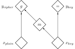
In this subsection we describe a family of bijective transformation with triangular Jacobian therefore tractable Jacobian determinant. That will serve a building block for the transformation $f$.

General coupling layer

Let $x\in{\mathcal{X}}$, $I_{1},I_{2}$ a partition of $\llbracket 1,D\rrbracket$ such that $d=\lvert I_{1}\rvert$ and $m$ a function defined on $\mathbb{R}^{d}$, we can define $y=(y_{I_{1}},y_{I_{2}})$ where:

$$y_{I_{1}} =x_{I_{1}}$$

$$y_{I_{2}} =g(x_{I_{2}};m(x_{I_{1}}))$$

where $g:\mathbb{R}^{D-d}\times m(\mathbb{R}^{d})\rightarrow\mathbb{R}^{D-d}$ is the coupling law, an invertible map with respect to its first argument given the second. The corresponding computational graph is shown Fig 2. If we consider $I_{1}=\llbracket 1,d\rrbracket$ and $I_{2}=\llbracket d,D\rrbracket$, the Jacobian of this function is:

$$\frac{\partial y}{\partial x}=\begin{bmatrix}I_{d}&0\\ \frac{\partial y_{I_{2}}}{\partial x_{I_{1}}}&\frac{\partial y_{I_{2}}}{\partial x_{I_{2}}}\end{bmatrix}$$

Where $I_{d}$ is the identity matrix of size $d$. That means that $\det\frac{\partial y}{\partial x}=\det\frac{\partial y_{I_{2}}}{\partial x_{I_{2}}}$. Also, we observe we can invert the mapping using:

$$x_{I_{1}} =y_{I_{1}}$$

$$x_{I_{2}} =g^{-1}(y_{I_{2}};m(y_{I_{1}}))$$

We call such a transformation a coupling layer with coupling function $m$.

Additive coupling layer

For simplicity, we choose as coupling law an additive coupling law $g(a;b)=a+b$ so that by taking $a=x_{I_{2}}$ and $b=m(x_{I_{1}})$:

$$y_{I_{2}} =x_{I_{2}}+m(x_{I_{1}})$$

$$x_{I_{2}} =y_{I_{2}}-m(y_{I_{1}})$$

and thus computing the inverse of this transformation is only as expensive as computing the transformation itself. We emphasize that there is no restriction placed on the choice of coupling function $m$ (besides having the proper domain and codomain). For example, $m$ can be a neural network with $d$ input units and $D-d$ output units.

Moreover, since $\det\frac{\partial y_{I_{2}}}{\partial x_{I_{2}}}=1$, an additive coupling layer transformation has a unit Jacobian determinant in addition to its trivial inverse. One could also choose other types of coupling, such as a multiplicative coupling law $g(a;b)=a\odot b,~{}b\neq 0$ or an affine coupling law $g(a;b)=a\odot b_{1}+b_{2},~{}b_{1}\neq 0$ if $m:{\mathbb{R}}^{d}\rightarrow{\mathbb{R}}^{D-d}\times{\mathbb{R}}^{D-d}$. We chose the additive coupling layer for numerical stability reason as the transformation become piece-wise linear when the coupling function, $m$, is a rectified neural network.

Combining coupling layers

We can compose several coupling layers to obtain a more complex layered transformation. Since a coupling layer leaves part of its input unchanged, we need to exchange the role of the two subsets in the partition in alternating layers, so that the composition of two coupling layers modifies every dimension. Examining the Jacobian, we observe that at least three coupling layers are necessary to allow all dimensions to influence one another. We generally use four.

3.3 Allowing rescaling

As each additive coupling layers has unit Jacobian determinant (i.e. is volume preserving), their composition will necessarily have unit Jacobian determinant too. In order to adress this issue, we include a diagonal scaling matrix $S$ as the top layer, which multiplies the $i$-th ouput value by $S_{ii}$: $(x_{i})_{i\leq D}\rightarrow(S_{ii}x_{i})_{i\leq D}$. This allows the learner to give more weight (i.e. model more variation) on some dimensions and less in others.

In the limit where $S_{ii}$ goes to $+\infty$ for some $i$, the effective dimensionality of the data has been reduced by $1$. This is possible so long as $f$ remains invertible around the data point. With such a scaled diagonal last stage along with lower triangular or upper triangular stages for the rest (with the identity in their diagonal), the NICE criterion has the following form:

$$\log(p_{X}(x))=\sum_{i=1}^{D}{\left[\log(p_{H_{i}}(f_{i}(x)))+\log(\lvert S_{ii}\rvert)\right]}.$$

We can relate these scaling factors to the eigenspectrum of a PCA, showing how much variation is present in each of the latent dimensions (the larger $S_{ii}$ is, the less important the dimension $i$ is). The important dimensions of the spectrum can be viewed as a manifold learned by the algorithm. The prior term encourages $S_{ii}$ to be small, while the determinant term $\log S_{ii}$ prevents $S_{ii}$ from ever reaching $0$.

3.4 Prior distribution

As mentioned previously, we choose the prior distribution to be factorial, i.e.:

$$p_{H}(h)=\prod_{d=1}^{D}{p_{H_{d}}(h_{d})}$$

We generally pick this distribution in the family of standard distribution, e.g. gaussian distribution:

$$\log(p_{H_{d}})=-\frac{1}{2}(h_{d}^{2}+\log(2\pi))$$

or logistic distribution:

$$\log(p_{H_{d}})=-\log(1+\exp(h_{d}))-\log(1+\exp(-h_{d}))$$

We tend to use the logistic distribution as it tends to provide a better behaved gradient.

4 Related methods

Significant advances have been made in generative models. Undirected graphical models like deep Boltzmann machines (DBM) (Salakhutdinov and Hinton,, 2009) have been very successful and an intense subject of research, due to efficient approximate inference and learning techniques that these models allowed. However, these models require Markov chain Monte Carlo (MCMC) sampling procedure for training and sampling and these chains are generally slowly mixing when the target distribution has sharp modes. In addition, the log-likelihood is intractable, and the best known estimation procedure, annealed importance sampling (AIS) (Salakhutdinov and Murray,, 2008), might yield an overly optimistic evaluation (Grosse et al.,, 2013).

Directed graphical models lack the conditional independence structure that allows DBMs efficient inference. Recently, however, the development of variational auto-encoders (VAE) (Kingma and Welling,, 2014; Rezende et al.,, 2014; Mnih and Gregor,, 2014; Gregor et al.,, 2014) - allowed effective approximate inference during training. In constrast with the NICE model, these approaches use a stochastic encoder $q(h\mid x)$ and an imperfect decoder $p(x\mid h)$, requiring a reconstruction term in the cost, ensuring that the decoder approximately inverts the encoder. This injects noise into the auto-encoder loop, since $h$ is sampled from $q(h\mid x)$, which is a variational approximation to the true posterior $p(h\mid x)$. The resulting training criterion is the variational lower bound on the log-likelihood of the data. The generally fast ancestral sampling technique that directed graphical models provide make these models appealing. Moreover, the importance sampling estimator of the log-likelihood is guaranteed not to be optimistic in expectation. But using a lower bound criterion might yield a suboptimal solution with respect to the true log-likelihood. Such suboptimal solutions might for example inject a significant amount of unstructured noise in the generation process resulting in unnatural-looking samples. In practice, we can output a statistic of $p(x\mid h)$, like the expectation or the median, instead of an actual sample. The use of a deterministic decoder can be motivated by the objective of eliminating low-level noise, which gets automatically added at the last stage of generation in models such as the VAE and Boltzmann machines (the visible are considered independent, given the hidden).

The NICE criterion is very similar to the criterion of the variational auto-encoder. More specifically, as the transformation and its inverse can be seen as a perfect auto-encoder pair (Bengio,, 2014), the reconstruction term is a constant that can be ignored. This leaves the Kullback-Leibler divergence term of the variational criterion: $log(p_{H}(f(x)))$ can be seen as the prior term, which forces the code $h=f(x)$ to be likely with respect to the prior distribution, and $\log(\lvert\det\frac{\partial f(x)}{\partial x}\rvert)$ can be seen as the entropy term. This entropy term reflects the local volume expansion around the data (for the encoder), which translates into contraction in the decoder $f^{-1}$. In a similar fashion, the entropy term in the variational criterion encourages the approximate posterior distribution to occupy volume, which also translates into contraction from the decoder. The consequence of perfect reconstruction is that we also have to model the noise at the top level, $h$, whereas it is generally handled by the conditional model $p(x\mid h)$ in these other graphical models.

We also observe that by combining the variational criterion with the reparametrization trick, (Kingma and Welling,, 2014) is effectively maximizing the joint log-likelihood of the pair $(x,\epsilon)$ in a NICE model with two affine coupling layers (where $\epsilon$ is the auxiliary noise variable) and gaussian prior, see Appendix C.

The change of variable formula for probability density functions is prominently used in inverse transform sampling (which is effectively the procedure used for sampling here). Independent component analysis (ICA) (Hyvärinen and Oja,, 2000), and more specifically its maximum likelihood formulation, learns an orthogonal transformation of the data, requiring a costly orthogonalization procedure between parameter updates. Learning a richer family of transformations was proposed in (Bengio,, 1991), but the proposed class of transformations, neural networks, lacks in general the structure to make the inference and optimization practical. (Chen and Gopinath,, 2000) learns a layered transformation into a gaussian distribution but in a greedy fashion and it fails to deliver a tractable sampling procedure.

(Rippel and Adams,, 2013) reintroduces this idea of learning those transformations but is forced into a regularized auto-encoder setting as a proxy of log-likelihood maximization due to the lack of bijectivity constraint. A more principled proxy of log-likelihood, the variational lower bound, is used more successfully in nonlinear independent components analysis (Hyvärinen and Pajunen,, 1999) via ensemble learning (Roberts and Everson,, 2001; Lappalainen et al.,, 2000) and in (Kingma and Welling,, 2014; Rezende et al.,, 2014) using a type of Helmholtz machine (Dayan et al.,, 1995). Generative adversarial networks (GAN) (Goodfellow et al.,, 2014) also train a generative model to transform a simple (e.g. factorial) distribution into the data distribution, but do not require an encoder that goes in the other direction. GAN sidesteps the difficulties of inference by learning a secondary deep network that discriminates between GAN samples and data. This classifier network provides a training signal to the GAN generative model, telling it how to make its output less distinguishable from the training data.

Like the variational auto-encoders, the NICE model uses an encoder to avoid the difficulties of inference, but its encoding is deterministic. The log-likelihood is tractable and the training procedure does not require any sampling (apart from dequantizing the data). The triangular structure used in NICE to obtain tractability is also present in another family of tractable density models, the neural autoregressive networks (Bengio and Bengio,, 2000), which include as a recent and succesful example the neural autoregressive density estimator (NADE) (Larochelle and Murray,, 2011). Indeed, the adjacency matrix in the NADE directed graphical model is strictly triangular. However the element-by-element autoregressive schemes make the ancestral sampling procedure computationally expensive and unparallelizable for generative tasks on high-dimensional data, such as image data. A NICE model using one coupling layer can be seen as a block version of NADE with two blocks.

5 Experiments

5.1 Log-likelihood and generation

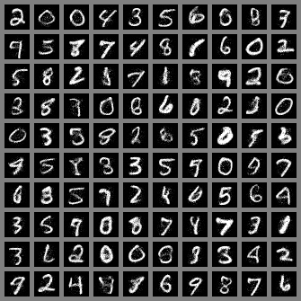
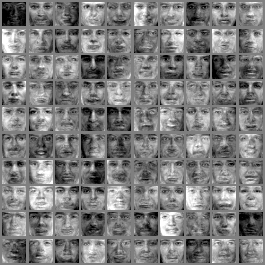
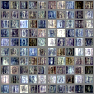
We train NICE on MNIST (LeCun and Cortes,, 1998), the Toronto Face Dataset (TFD) (Susskind et al.,, 2010), the Street View House Numbers dataset (SVHN) (Netzer et al.,, 2011) and CIFAR-10 (Krizhevsky,, 2010). As prescribed in (Uria et al.,, 2013), we use a dequantized version of the data: we add a uniform noise of $\frac{1}{256}$ to the data and rescale it to be in $[0,1]^{D}$ after dequantization. We add a uniform noise of $\frac{1}{128}$ and rescale the data to be in $[-1,1]^{D}$ for CIFAR-10.

The architecture used is a stack of four coupling layers with a diagonal positive scaling (parametrized exponentially) $\exp(s)$ for the last stage, and with an approximate whitening for TFD and exact ZCA on SVHN and CIFAR-10. We partition the input space between by separating odd ($I_{1}$) and even ($I_{2}$) components, so the equation is:

$$h^{(1)}_{I_{1}} =x_{I_{1}}$$

$$h^{(1)}_{I_{2}} =x_{I_{2}}+m^{(1)}(x_{I_{1}})$$

$$h^{(2)}_{I_{2}} =h^{(1)}_{I_{2}}$$

$$h^{(2)}_{I_{1}} =h^{(1)}_{I_{1}}+m^{(2)}(x_{I_{2}})$$

$$h^{(3)}_{I_{1}} =h^{(2)}_{I_{1}}$$

$$h^{(3)}_{I_{2}} =h^{(2)}_{I_{2}}+m^{(3)}(x_{I_{1}})$$

$$h^{(4)}_{I_{2}} =h^{(3)}_{I_{2}}$$

$$h^{(4)}_{I_{1}} =h^{(3)}_{I_{1}}+m^{(4)}(x_{I_{2}})$$

$$h=\exp(s)\odot h^{(4)}$$

The coupling functions $m^{(1)},m^{(2)},m^{(3)}$ and $m^{(4)}$ used for the coupling layers are all deep rectified networks with linear output units. We use the same network architecture for each coupling function: five hidden layers of $1000$ units for MNIST, four of $5000$ for TFD, and four of $2000$ for SVHN and CIFAR-10.

Dataset	MNIST	TFD	SVHN	CIFAR-10
# dimensions	$784$	$2304$	$3072$	$3072$
Preprocessing	None	Approx. whitening	ZCA	ZCA
# hidden layers	$5$	$4$	$4$	$4$
# hidden units	$1000$	$5000$	$2000$	$2000$
Prior	logistic	gaussian	logistic	logistic
Log-likelihood	$1980.50$	$5514.71$	$11496.55$	$5371.78$

Figure 3: Architecture and results. # hidden units refer to the number of units per hidden layer.

Model	TFD	CIFAR-10
NICE	$5514.71$	$5371.78$
Deep MFA	$5250$	$3622$
GRBM	$2413$	$2365$

Figure 4: Log-likelihood results on TFD and CIFAR-10. Note that the Deep MFA number correspond to the best results obtained from (Tang et al.,, 2012) but are actually variational lower bound.

A standard logistic distribution is used as prior for MNIST, SVHN and CIFAR-10. A standard normal distribution is used as prior for TFD.

The models are trained by maximizing the log-likelihood $\log(p_{H}(h))+\sum_{i=1}^{D}{s_{i}}$ with AdaM (Kingma and Ba,, 2014) with learning rate $10^{-3}$, momentum $0.9$, $\beta_{2}=0.01$, $\lambda=1$, and $\epsilon=10^{-4}$. We select the best model in terms of validation log-likelihood after $1500$ epochs.

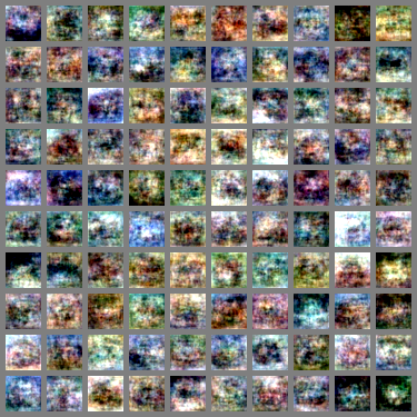
We obtained a test log-likelihood of $1980.50$ on MNIST, $5514.71$ on TFD, $11496.55$ for SVHN and $5371.78$ for CIFAR-10. This compares to the best results that we know of in terms of log-likelihood: $5250$ on TFD and $3622$ on CIFAR-10 with deep mixtures of factor analysers (Tang et al.,, 2012) (although it is still a lower bound), see Table 4. As generative models on continuous MNIST are generally evaluated with Parzen window estimation, no fair comparison can be made. Samples generated by the trained models are shown in Fig. 5.

(a) Model trained on MNIST

(b) Model trained on TFD

(c) Model trained on SVHN

(d) Model trained on CIFAR-10

Figure 5: Unbiased samples from a trained NICE model. We sample $h\sim p_{H}(h)$ and we output $x=f^{-1}(h)$.

5.2 Inpainting

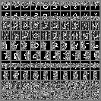
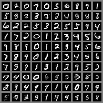
Here we consider a naive iterative procedure to implement inpainting with the trained generative models. For inpainting we clamp the observed dimensions $(x_{O})$ to their values and maximize log-likelihood with respect to the hidden dimensions $(X_{H})$ using projected gradient ascent (to keep the input in its original interval of values) with gaussian noise with step size $\alpha_{i}=\frac{10}{100+i}$, where $i$ is the iteration, following the stochastic gradient update:

$$x_{H,i+1} =x_{H,i}+\alpha_{i}(\frac{\partial\log(p_{X}((x_{O},x_{H,i})))}{\partial x_{H,i}}+\epsilon)$$

$$\epsilon \sim{\mathcal{N}}(0,I)$$

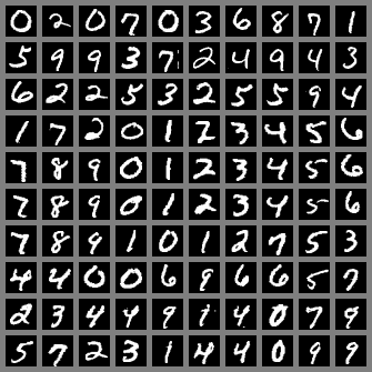
where $x_{H,i}$ are the values of the hidden dimensions at iteration $i$. The result is shown on test examples of MNIST, in Fig 6. Although the model is not trained for this task, the inpainting procedure seems to yield reasonable qualitative performance, but note the occasional presence of spurious modes.

(a) MNIST test examples

(b) Initial state

(c) MAP inference of the state

Figure 6: Inpainting on MNIST. We list below the type of the part of the image masked per line of the above middle figure, from top to bottom: top rows, bottom rows, odd pixels, even pixels, left side, right side, middle vertically, middle horizontally, 75% random, 90% random. We clamp the pixels that are not masked to their ground truth value and infer the state of the masked pixels by projected gradient ascent on the likelihood. Note that with middle masks, there is almost no information available about the digit.

6 Conclusion

In this work we presented a new flexible architecture for learning a highly non-linear bijective transformation that maps the training data to a space where its distribution is factorized, and a framework to achieve this by directly maximizing log-likelihood. The NICE model features efficient unbiased ancestral sampling and achieves competitive results in terms of log-likelihood.

Note that the architecture of our model could be trained using other inductive principles capable of exploiting its advantages, like toroidal subspace analysis (TSA) (Cohen and Welling,, 2014).

We also briefly made a connection with variational auto-encoders. We also note that NICE can enable more powerful approximate inference allowing a more complex family of approximate posterior distributions in those models, or a richer family of priors.

Appendix A Further Visualizations

A.1 Manifold visualization

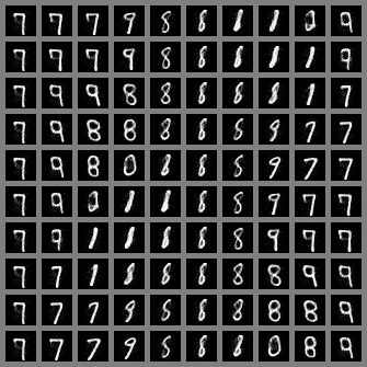
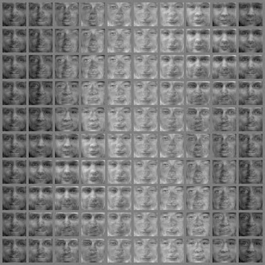
To illustrate the learned manifold, we also take a random rotation $R$ of a 3D sphere $S$ in latent space and transform it to data space, the result $f^{-1}(R(S))$ is shown in Fig 7.

A.2 Spectrum

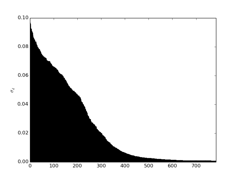
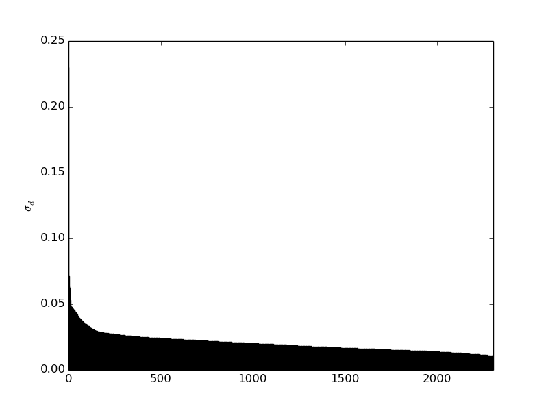
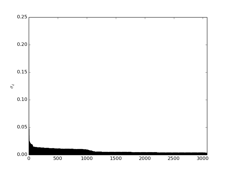
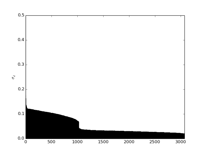
We also examined the last diagonal scaling layer and looked at its coefficients $(S_{dd})_{d\leq D}$. If we consider jointly the prior distribution and the diagonal scaling layer, $\sigma_{d}=S_{dd}^{-1}$ can be considered as the scale parameter of each independent component. This shows us the importance that the model has given to each component and ultimately how successful the model was at learning manifolds. We sort $(\sigma_{d})_{d\leq D}$ and plot it in Fig 8.

(a) Model trained on MNIST

(b) Model trained on TFD

Figure 7: Sphere in the latent space. These figures show part of the manifold structure learned by the model.

(a) Model trained on MNIST

(b) Model trained on TFD

(c) Model trained on SVHN

(d) Model trained on CIFAR-10

Figure 8: Decay of $\sigma_{d}=S_{dd}^{-1}$. The large values correspond to dimensions on which the model chooses to have larger variations, thus highlighting the learned manifold structure from the data. This is the non-linear equivalent of the eigenspectrum in the case of PCA. On the x axis are the components $d$ sorted by $\sigma_{d}$ (on the y axis).

Appendix B Approximate whitening

The procedure for learning the approximate whitening is using the NICE framework, with an affine function and a standard gaussian prior. We have:

$$z=Lx+b$$

with $L$ lower triangular and $b$ a bias vector. This is equivalent to learning a gaussian distribution. The optimization procedure is the same as NICE: RMSProp with early stopping and momentum.

Appendix C Variational auto-encoder as NICE

We assert here that the stochastic gradient variational Bayes (SGVB) algorithm maximizes the log-likelihood on the pair $(x,\epsilon).$(Kingma and Welling,, 2014) define a recognition network:

$$z=g_{\phi}(\epsilon\mid x),~{}\epsilon\sim{\mathcal{N}}(0,I)$$

For a standard gaussian prior $p(z)$ and conditional $p(x\mid z)$, we can define:

$$\xi=\frac{x-f_{\theta}(z)}{\sigma}$$

If we define a standard gaussian prior on $h=(z,\xi)$. The resulting cost function is:

$$\log(p_{(x,\epsilon),(\theta,\phi)}(x,\epsilon))=\log(p_{H}(h))-D_{X}\log(\sigma)+\log(\lvert\det\frac{\partial g_{\phi}}{\partial\epsilon}(\epsilon;x)\rvert)$$

with $D_{X}=dim(X)$. This is equivalent to:

$$\log(p_{(x,\epsilon),(\theta,\phi)}(x,\epsilon))-\log(p_{\epsilon}(\epsilon)) =\log(p_{H}(h))-D_{X}\log(\sigma)+\log(\lvert\det\frac{\partial g_{\phi}}{\partial\epsilon}(\epsilon;x)\rvert)-\log(p_{\epsilon}(\epsilon))$$

$$=\log(p_{H}(h))-D_{X}\log(\sigma)-\log(q_{Z\mid X;\phi}(z))$$

$$=\log(p_{\xi}(\xi)p_{Z}(z))-D_{X}\log(\sigma)-\log(q_{Z\mid X;\phi}(z))$$

$$=\log(p_{\xi}(\xi))+\log(p_{Z}(z))-D_{X}\log(\sigma)-\log(q_{Z\mid X;\phi}(z))$$

$$=\log(p_{\xi}(\xi))-D_{X}\log(\sigma)+\log(p_{Z}(z))-\log(q_{Z\mid X;\phi}(z))$$

$$=\log(p_{X\mid Z}(x\mid z))+\log(p_{Z}(z))-\log(q_{Z\mid X;\phi}(z))$$

This is the Monte Carlo estimate of the SGVB cost function proposed in (Kingma and Welling,, 2014).

References

- Bastien et al., (2012) Bastien, F., Lamblin, P., Pascanu, R., Bergstra, J., Goodfellow, I. J., Bergeron, A., Bouchard, N., and Bengio, Y. (2012). Theano: new features and speed improvements. Deep Learning and Unsupervised Feature Learning NIPS 2012 Workshop.
- Bengio, (1991) Bengio, Y. (1991). Artificial Neural Networks and their Application to Sequence Recognition. PhD thesis, McGill University, (Computer Science), Montreal, Canada.
- Bengio, (2009) Bengio, Y. (2009). Learning deep architectures for AI. Now Publishers.
- Bengio, (2014) Bengio, Y. (2014). How auto-encoders could provide credit assignment in deep networks via target propagation. Technical report, arXiv:1407.7906.
- Bengio and Bengio, (2000) Bengio, Y. and Bengio, S. (2000). Modeling high-dimensional discrete data with multi-layer neural networks. In Solla, S., Leen, T., and Müller, K.-R., editors, Advances in Neural Information Processing Systems 12 (NIPS’99), pages 400–406. MIT Press.
- Bengio et al., (2013) Bengio, Y., Mesnil, G., Dauphin, Y., and Rifai, S. (2013). Better mixing via deep representations. In Proceedings of the 30th International Conference on Machine Learning (ICML’13). ACM.
- Bergstra et al., (2011) Bergstra, J., Bastien, F., Breuleux, O., Lamblin, P., Pascanu, R., Delalleau, O., Desjardins, G., Warde-Farley, D., Goodfellow, I. J., Bergeron, A., and Bengio, Y. (2011). Theano: Deep learning on gpus with python. In Big Learn workshop, NIPS’11.
- Chen and Gopinath, (2000) Chen, S. S. and Gopinath, R. A. (2000). Gaussianization.
- Cohen and Welling, (2014) Cohen, T. and Welling, M. (2014). Learning the irreducible representations of commutative lie groups. arXiv:1402.4437.
- Dayan et al., (1995) Dayan, P., Hinton, G. E., Neal, R., and Zemel, R. (1995). The Helmholtz machine. Neural Computation, 7:889–904.
- Goodfellow et al., (2014) Goodfellow, I. J., Pouget-Abadie, J., Mirza, M., Xu, B., Warde-Farley, D., Ozair, S., Courville, A., and Bengio, Y. (2014). Generative adversarial networks. Technical Report arXiv:1406.2661, arxiv.
- Goodfellow et al., (2013) Goodfellow, I. J., Warde-Farley, D., Lamblin, P., Dumoulin, V., Mirza, M., Pascanu, R., Bergstra, J., Bastien, F., and Bengio, Y. (2013). Pylearn2: a machine learning research library. arXiv preprint arXiv:1308.4214.
- Gregor et al., (2014) Gregor, K., Danihelka, I., Mnih, A., Blundell, C., and Wierstra, D. (2014). Deep autoregressive networks. In International Conference on Machine Learning (ICML’2014).
- Grosse et al., (2013) Grosse, R., Maddison, C., and Salakhutdinov, R. (2013). Annealing between distributions by averaging moments. In ICML’2013.
- Hyvärinen and Oja, (2000) Hyvärinen, A. and Oja, E. (2000). Independent component analysis: algorithms and applications. Neural networks, 13(4):411–430.
- Hyvärinen and Pajunen, (1999) Hyvärinen, A. and Pajunen, P. (1999). Nonlinear independent component analysis: Existence and uniqueness results. Neural Networks, 12(3):429–439.
- Kingma and Ba, (2014) Kingma, D. and Ba, J. (2014). Adam: A method for stochastic optimization. arXiv preprint arXiv:1412.6980.
- Kingma and Welling, (2014) Kingma, D. P. and Welling, M. (2014). Auto-encoding variational bayes. In Proceedings of the International Conference on Learning Representations (ICLR).
- Krizhevsky, (2010) Krizhevsky, A. (2010). Convolutional deep belief networks on CIFAR-10. Technical report, University of Toronto. Unpublished Manuscript: http://www.cs.utoronto.ca/ kriz/conv-cifar10-aug2010.pdf.
- Lappalainen et al., (2000) Lappalainen, H., Giannakopoulos, X., Honkela, A., and Karhunen, J. (2000). Nonlinear independent component analysis using ensemble learning: Experiments and discussion. In Proc. ICA. Citeseer.
- Larochelle and Murray, (2011) Larochelle, H. and Murray, I. (2011). The Neural Autoregressive Distribution Estimator. In Proceedings of the Fourteenth International Conference on Artificial Intelligence and Statistics (AISTATS’2011), volume 15 of JMLR: W&CP.
- LeCun and Cortes, (1998) LeCun, Y. and Cortes, C. (1998). The mnist database of handwritten digits.
- Mnih and Gregor, (2014) Mnih, A. and Gregor, K. (2014). Neural variational inference and learning in belief networks. In ICML’2014.
- Netzer et al., (2011) Netzer, Y., Wang, T., Coates, A., Bissacco, A., Wu, B., and Ng, A. Y. (2011). Reading digits in natural images with unsupervised feature learning. Deep Learning and Unsupervised Feature Learning Workshop, NIPS.
- Ozair and Bengio, (2014) Ozair, S. and Bengio, Y. (2014). Deep directed generative autoencoders. Technical report, U. Montreal, arXiv:1410.0630.
- Rezende et al., (2014) Rezende, D. J., Mohamed, S., and Wierstra, D. (2014). Stochastic backpropagation and approximate inference in deep generative models. Technical report, arXiv:1401.4082.
- Rippel and Adams, (2013) Rippel, O. and Adams, R. P. (2013). High-dimensional probability estimation with deep density models. arXiv:1302.5125.
- Roberts and Everson, (2001) Roberts, S. and Everson, R. (2001). Independent component analysis: principles and practice. Cambridge University Press.
- Salakhutdinov and Hinton, (2009) Salakhutdinov, R. and Hinton, G. (2009). Deep Boltzmann machines. In Proceedings of the International Conference on Artificial Intelligence and Statistics, volume 5, pages 448–455.
- Salakhutdinov and Murray, (2008) Salakhutdinov, R. and Murray, I. (2008). On the quantitative analysis of deep belief networks. In Cohen, W. W., McCallum, A., and Roweis, S. T., editors, Proceedings of the Twenty-fifth International Conference on Machine Learning (ICML’08), volume 25, pages 872–879. ACM.
- Susskind et al., (2010) Susskind, J., Anderson, A., and Hinton, G. E. (2010). The Toronto face dataset. Technical Report UTML TR 2010-001, U. Toronto.
- Tang et al., (2012) Tang, Y., Salakhutdinov, R., and Hinton, G. (2012). Deep mixtures of factor analysers. arXiv preprint arXiv:1206.4635.
- Uria et al., (2013) Uria, B., Murray, I., and Larochelle, H. (2013). Rnade: The real-valued neural autoregressive density-estimator. In NIPS’2013.