On the Degree Distribution of Pólya Urn Graph Processes

Abstract

This paper presents a tighter bound on the degree distribution of arbitrary Pólya urn graph processes, proving that the proportion of vertices with degree $d$ obeys a power-law distribution $P(d)\propto d^{-\gamma}$ for $d\leq n^{\nicefrac{{1}}{{6}}-\epsilon}$ for any $\epsilon>0$, where $n$ represents the number of vertices in the network. Previous work by Bollobás et al.formalized the well-known preferential attachment model of Barabási and Albert, and showed that the power-law distribution held for $d\leq n^{\nicefrac{{1}}{{15}}}$ with $\gamma=3$. Our revised bound represents a significant improvement over existing models of degree distribution in scale-free networks, where its tightness is restricted by the Azuma-Hoeffding concentration inequality for martingales. We achieve this tighter bound through a careful analysis of the first set of vertices in the network generation process, and show that the newly acquired is at the edge of exhausting Bollobás model in the sense that the degree expectation breaks down for other powers.

1 Introduction

The power-law degree distribution is an interesting property exhibited by many complex networks. Aiming at a better understanding of such a characteristic, Barabási and Albert proposed a linear preferential attachment model for generating scale-free networks [2]. The definition of their process, however, was rather informal, as noted by Durret [11]. Since then, different precise forms of such a formulation have been studied in literature [15, 16, 17]. Out of these, the Bollobás et al.model [9], adopted in this paper, stands out as it has been at the core of various developments in network studies [7, 10, 19, 20]. Further, Bollobás et al.’s approach is quite general, as opposed to alternative interpretations [13], in the sense that the degree distribution is size dependent.

In their approach, Bollobás et al.introduce $n$-pairings (i.e., linear chord diagram models) as the procedure to formalize the preferential attachment process. Interestingly, this method allows for the definition of random graphs over $n$ vertices non-recursively. The model also allows for both loops and multiple edges. The authors prove that the power-law degree distribution can be acquired with $\gamma=3$. The proof, however, operates only when the studied degree $d\leq n^{\nicefrac{{1}}{{15}}}$. Such loose bounds restrict real-world applications of Bollobá’s theorem [9] due to the need for extremely large networks (e.g., $10^{15}$ for an individual degree of $10$).

Aiming at a more realistic setting, this paper contributes by first tightening the degree distribution bound above from $d\leq n^{\nicefrac{{1}}{{15}}}$ to $d\leq n^{\nicefrac{{1}}{{14}}-\epsilon}$ for any $\epsilon>0$. Although successful, we show that this result can be further constricted. We introduce a careful analysis of the first set of vertices in the network generation process and show that the bound can be further improved to $d\leq n^{\nicefrac{{1}}{{6}}-\epsilon}$ for any $\epsilon>0$. To our knowledge, this is the tightest bound for the degree distribution of scale-free networks in such a general setting discovered so far. Finally, we present a corollary of the second theorem demonstrating that the newly acquired bound is tight to changes in degree exponents.

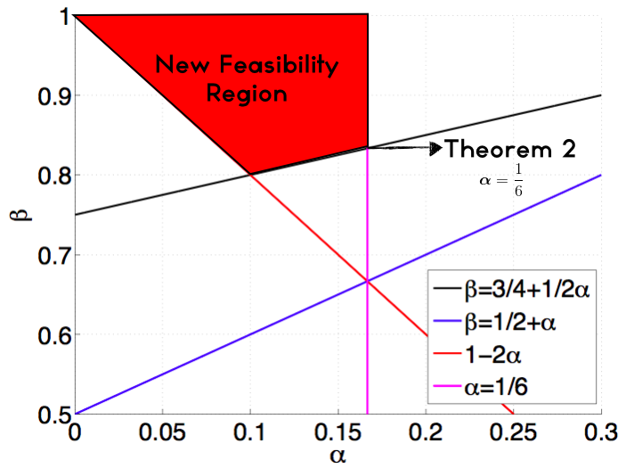
Our final results provide an improvement over previous work, showing that the degree distribution of vertices in arbitrary networks following from the preferential attachment process obey a power-law distribution $P(d)\propto d^{-\gamma}$ for $d\leq n^{\nicefrac{{1}}{{6}}-\epsilon}$ for any $\epsilon>0$. To illustrate, the set of inequalities attained for determining the exponents of the number of vertices are plotted for both theorems proved in this paper. In Figure 2, we show the extend to which Bollobá’s method can be stretched without the careful analysis of the first set of vertices, leading to an exponent of $\nicefrac{{1}}{{14}}$. After our careful analysis of the first set of vertices, we are capable of further extending that feasibility region to acquire an exponent of $\nicefrac{{1}}{{6}}$, see Figure 2.

Figure 1: An illustration showing the result attained in Theorem 1, where Bollobá’s bound is tightened from $\nicefrac{{1}}{{15}}$ to $\nicefrac{{1}}{{14}}$.

Figure 2: Illustrating the extension of the feasibility region due to our analysis in Theorem 2, being at the edge of exhausting Bollobá’s method.

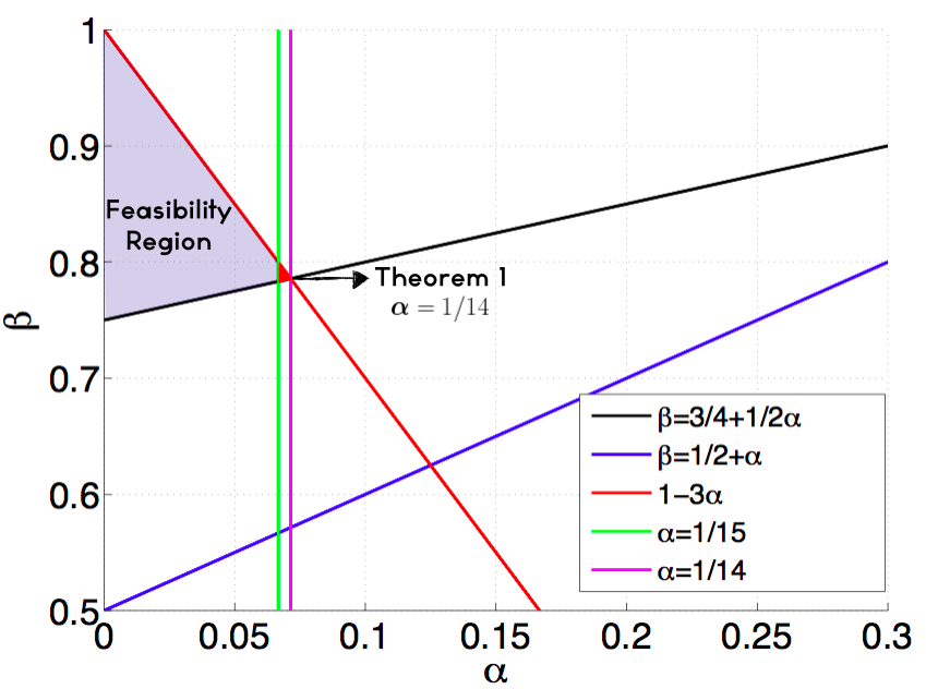
This newly acquired bound can be considered tight as its tightness is restricted by the Azuma-Hoeffding concentration inequality for martingales. Our approach is also at the edge of exhausting Bollobás et al.’s approach, in the sense that the degree expectation breaks down for other powers.

2 Background

2.1 Preferential Attachment and the Pólya Urn Process

The preferential attachment process introduced in [2] can be formalized as a combination of Pólya urn processes [21], in the sense that each newly arriving connection can represent a new ball added to the urn corresponding to that vertex. For such a formalization, consider a Pólya urn process with a two urn model, where the number of balls in one urn represent the degree of a node $\bm{v}_{k}$, and those in the second denote the sum of the degrees for $\bm{v}_{1},\dots,\bm{v}_{k-1}$. The process starts at $n=k$, where node $\bm{v}_{k}$ has exactly $m>0$ connections to $\bm{v}_{1},\dots,\bm{v}_{k-1}$. Recognizing that at this stage the first and second urns start with $m$ and $\left(2k-3\right)m$ balls, respectively, it is easy to see that the evolution is a Pólya urn with strengths $\bm{\alpha}_{k}$ and $1-\bm{\alpha}_{k}$ with $\bm{\alpha}_{k}\sim\bm{\beta}\left(m,\left(2k-3\right)m\right)$, with $\bm{\beta}(\cdot)$ representing the Beta distribution.

The aforementioned process enables an accurate definition of the preferential attachment model by setting $\bm{\alpha}_{1}=1$, and for $2\leq k\leq n$, $\bm{\alpha}_{k}\sim\bm{\beta}\left(m,\left(2k-3\right)m\right)$. Further, by letting $\bm{l}_{k}=\sum_{j=1}^{k}\bm{\Phi}_{k}$, with $\bm{\Phi}_{k}=\bm{\alpha}_{k}\prod_{j=k+1}^{n}\left(1-\bm{\alpha}_{j}\right)$ for $1\leq k\leq n$, an edge between $\bm{v}_{k}$ and $\bm{v}_{j}$ is drawn if for some $i\in[1,m]$, we have $j=\bm{\kappa}\left(\bm{U}_{i,k}\bm{l}_{k-1}\right)$, with $\bm{\kappa}\left(a\right)=\min\left\{k:\bm{l}_{k}\geq a\right\}$ for $a\in[0,1]$ and $\left\{\bm{U}_{i,k}\right\}$ being a sequence of independent random variables for $1\leq i\leq m$ and $1\leq k\leq n$.

Though appealing, Bollobás et al. [9], among others, presented a procedure to formalize such preferential attachment models based on the concept of $n$-pairings [6, 8] enabling easier analysis. This framework exhibits multiple advantages, such as constructing graphs over $n$ vertices non-recursively, and providing compact and tractable representations of degree distributions. Furthermore, this method has been at the core of multiple alternative formalizations of preferential attachment [7, 10, 19, 20] and therefore we adopt it in this paper as a general framework in the study of the degree distribution of scale-free networks.

2.2 $n$-Pairings and Graph Generation

The idea of $n$-parings [8, 6] is one of the essential steps required to generate graphs in the formalization introduced by Bollobás et al. [9]. An n-pairing is a partition of the set $\{1,2,\dots,2n\}$ into pairs, so there are $\left(2n-1\right)!!=\nicefrac{{(2n)!}}{{\left(n!2^{n}\right)}}$ $n$-pairings [9]. These objects can be viewed as linearized chord diagrams (LCDs) [8]. An LCD with $n$ chords consists of $2n$ distinct points on the x-axis paired by chords.

Starting from $2n$-nodes, this process first generates a random matching between pairs of nodes. A directed graph $\bm{\Psi}\left(\mathcal{P}\right)$ is then formed from an $n$-pairing $\mathcal{P}$ as follows: starting from the left, merge all endpoints including the first right endpoint to form $v_{1}$. At this stage, merge all further endpoints up to the next right endpoint to form $v_{2}$. This procedure is repeated until it reaches $v_{n}$. Edges are created by replacing each pair by a directed edge from the vertex corresponding to its right endpoint to that corresponding to its left endpoint. As noted by Bollobás et al. [9], if $\mathcal{P}$ is chosen uniformly at random from all $\nicefrac{{(2n)!}}{{\left(n!2^{n}\right)}}$ $n$-pairings, then $\bm{\Psi}\left(\mathcal{P}\right)$ has the same distribution as a random graph. Such a process can be used to formalize the widely known preferential attachment model of Barabási and Albert, as detailed next.

2.3 Generating Graphs

Bollobás introduced two processes to formalize the scale-free degree distribution inherent to real-world networks. In the one-connection preferential attachment process (Section 2.3.1) the goal is for a new node to make just one connection to the existing nodes in the graph. The multiple-connections preferential attachment process (Section 2.3.2), generalizes this idea to $m>1$ connections. In this setting, the graphs are created by applying the one-connection process multiple times.

2.3.1 One-Connection Preferential Attachment Process

For $m=1$, the goal is for each new node to make only one connection to those nodes that already exist in the graph. This process, $\left(\mathbb{G}_{1}^{(n)}\right)_{n\geq 0}$, is defined inductively so that $\mathbb{G}_{1}^{(n)}$ is a directed graph on $\{v_{i}:1\leq i\leq n\}$. Formally:

Definition 1 (One-Connection Preferential Attachment Process [9]:).

Start with $\mathbb{G}_{1}^{(1)}$, the graph with one vertex and one loop. Construct $\mathbb{G}_{1}^{(n)}$ from $\mathbb{G}_{1}^{(n-1)}$ by adding a vertex (node) $v_{n}$ with a single directed edge from $v_{n}$ to $v_{i}$, with $i$ chosen according to:

$$\mathbb{P}\mathrm{r}(i=s)=\left\{\begin{array}[]{ll}\frac{d^{\left(\mathbb{G}_{1}^{(n-1)}\right)}[v_{s}]}{2n-1}&:1\leq s\leq n-1\\ \nicefrac{{1}}{{2n-1}}&:s=t\end{array}\right.\enspace.$$

2.3.2 Multiple-Connections Preferential Attachment Process

For the case of $m>1$ (i.e., multiple connections), $m$ edges from the new node are added one at a time. The process $\left(\mathbb{G}^{(n)}_{m}\right)_{n\geq 0}$ is defined as following:

Definition 2 (Multiple-Connections Preferential Attachment Process [9]:).

The process $\left(\mathbb{G}^{(n)}_{m}\right)_{n\geq 0}$ is defined by running $\left(\mathbb{G}^{(n)}_{1}\right)_{n\geq 0}$ on a set of vertices $v^{\prime}_{1},v^{\prime}_{2}\dots$ to create $\mathbb{G}^{(mn)}_{1}$. The graph $\mathbb{G}^{(n)}_{m}$ is then formed by identifying the vertices $v_{1}^{\prime},\dots,v^{\prime}_{m}$ to form $v_{1}$, $v^{\prime}_{m+1},\dots,v^{\prime}_{2m}$ to form $v_{2}$, and so forth.

The probability space for directed graphs on $n$ vertices will be denoted by $\mathcal{G}_{m}^{(n)}$, where $\mathbb{G}_{m}^{(n)}\in\mathcal{G}_{m}^{(n)}$ has the distribution derived from the multiple-connection preferential attachment process described above. As noted by Bollobás and Riordan [8], such a distribution has an alternative description in terms of $n$-pairings with the advantage of a simple and non-recursive definition of the distribution of $\mathbb{G}_{m}^{(n)}$. Due to space constraints, the details of such derivations are omitted in this paper. Interested readers are referred to either the supplementary material accompanying this paper or to Bollobás et al.[9, 8] for a more thorough explanation.

3 Revised Bounds on the Degree Distribution

This section presents the main results of this paper in the form of two theorems. Due to space constraints, we only provide proof sketches here; extended proofs can be found in the supplementary material accompanying this paper. Theorem 1 tightens the bounds on the in-degree distribution of scale-free networks from $n^{\nicefrac{{1}}{{15}}}$ to $n^{\nicefrac{{1}}{{14}}-\epsilon}$ for any $\epsilon>0$. Our second main result, summarized in Theorem 2, further tightens the above bound to attain $n^{\nicefrac{{1}}{{6}}-\epsilon}$ for any $\epsilon>0$. This bound is the tightest discovered for such a general setting so far. We achieve $n^{\nicefrac{{1}}{{6}}-\epsilon}$ by performing a detailed and careful analysis of the degree distribution of the first set of vertices in scale-free networks.

Theorem 1.

Let $m\geq 1$ be fixed and $\left(\mathbb{G}_{m}^{(n)}\right)_{n\geq 0}$ be the process defined in Section 2.3.2. For any $\epsilon>0$ and $1\leq d\leq n^{\nicefrac{{1}}{{14}}-\epsilon}$:

$$\mathbb{P}\mathrm{r}\left[\frac{N\left(n,m,d\right)}{n}\sim\frac{1}{d^{3}}\right]\rightarrow 1,\ \text{as $n\rightarrow\infty$}\enspace,$$

with $N\left(n,m,d\right)$ being the number of vertices in graph $\mathbb{G}_{m}^{(n)}$ with an in-degree $d$.

Intuitively, the above theorem states that the probability for vertices to follow a power-law distribution tends to 1 as the $n$ grows large. The studied degree, in this case, should be restricted in the range of $1\leq d\leq n^{\nicefrac{{1}}{{14}}-\epsilon}$ for some $\epsilon>0$, which is tighter than that derived by Bollobás et al.[9] (i.e., $1\leq d\leq n^{\nicefrac{{1}}{{15}}}$). Note that later, we further tighten this bound to $n^{\nicefrac{{1}}{{6}}-\epsilon}$ as summarized by Theorem 2.

Proof.

Our proof is closely related to that of Bollobás et al.[9] with major differences including the tightness of the derived bounds. At a high level, the proof is performed in two steps. In the first step, we consider the $m=1$ scenario and then generalize to $m>1$. Considering $m=1$, the proof is established by proving three Lemmas.

First, we will prove the following:

Lemma 1.

Let $D_{k}$ be the sum of the total degrees of nodes $v_{1},v_{2},\ldots v_{k}$ in graph $\mathbb{G}^{(n)}_{1}$. Then,

$$\mathbb{P}\mathrm{r}\left[|D_{k}-2\sqrt{4kn}|\geq 4\sqrt{n\log n}\right]\approx\mathcal{O}(n^{-\nicefrac{{7}}{{4}}})\enspace.$$

Proof.

Fixing $1\leq s\leq n-k$, we bound the probability of the event $\bm{A}=\{D_{k}=2k+s\}$. The event $\bm{A}$ is equivalent to the event that a set of new nodes $\left(\text{i.e.,}\{v_{k+1},v_{k+2},\ldots,v_{n}\}\right)$ makes exactly $s$ links with the collection $\{v_{1},v_{2},\ldots,v_{k}\}$. This is true since in the $\mathbb{G}^{(n)}_{1}$ process each new node creates exactly one outgoing link with previous nodes. Precisely, $\{v_{1},v_{2},\ldots,v_{k}\}$ exhibit exactly $k$ edges among themselves.

To acquire the value of $\mathbb{P}\mathrm{r}[\bm{A}]$, we will use a well-know result from the $n$-pairings theory [8]. Namely, if $n$-pairings are chosen uniformly randomly, then the corresponding directed graph will exhibit the same distribution as $\mathbb{G}^{(n)}_{1}$:

$$\mathbb{P}\mathrm{r}\left[\bm{A}\right]=\frac{N(s)}{(2n-1)!!}\enspace,$$ (1)

with $N(s)$ representing the number of $n$-pairings in which the $k^{th}$ right-end point corresponds to the LCD-node $2k+s$, with exactly $s$ LCD-nodes in the collection $C_{\text{left}}\triangleq\{1,2,\ldots 2k+s\}$ being left end-points for some $s$ nodes in the collection $C_{\text{right}}\triangleq\{2k+s+1,2k+s+2,\ldots 2n\}$. Furthermore, the total number of all $n$-pairings is given by $(2n-1)!!=\nicefrac{{(2n)!}}{{2^{n}n!}}$. Notice that the number of ways to pair LCD-node $2k+s$ with: (1) one of the elements in $C_{\text{left}}$, and (2) exactly $2k-s-2$ elements of $C_{\text{left}}$ with themselves is given by $(2k+s-1)\left(\begin{array}[]{c}2k+s-2\\ s\end{array}\right)(2k-2)!!$. Similarly, the number of ways to pair exactly $(2n-2k-2s)$ numbers of $C_{\text{right}}$ among each other is given by $\left(\begin{array}[]{c}2n-2k-s\\ s\end{array}\right)(2n-2k-2s)!!$.

Having these derivations, we can write:

$$N(s)=s!(2k+s-1)\left(\begin{array}[]{c}2k+s-2\\ s\end{array}\right)(2k-2)!!\left(\begin{array}[]{c}2n-2k-s\\ s\end{array}\right)(2n-2k-2s)!!\enspace,$$

with $s!$ representing all different ways in which $s$ $C_{\text{left}}$ LCD-nodes can be paired with $s$ nodes in $C_{\text{right}}$.

Given this result, we can rewrite Equation 1 as:

$$\mathbb{P}\mathrm{r}\left[\bm{A}\right]=\frac{(2k+s-1)!(2n-2k-s)!n!2^{s+1}}{s!(k-1)!(n-k-s)!(2n)!}\enspace.$$ (2)

Note that for a fixed $k$, the function $f(s)=\nicefrac{{\mathbb{P}\mathrm{r}\left[D_{k}=2k+s+1\right]}}{{\mathbb{P}\mathrm{r}\left[D_{k}=2k+s\right]}}=\nicefrac{{2(2k+s)(n-k-s)}}{{(s+1)(2n-2k-s)}}$ decreases with $s$. Considering the case where $\nicefrac{{2(2k+s)(n-k-s)}}{{(s+1)(2n-2k-s)}}=1$, we have the following solutions for $s$:

$$s_{01}=\lceil-2k+\sqrt{4kn-2n+\nicefrac{{1}}{{4}}}+\nicefrac{{1}}{{2}}\rceil\enspace,$$

$$s_{02}=\lfloor-2k-\sqrt{4kn-2n+\nicefrac{{1}}{{4}}}-\nicefrac{{1}}{{2}}\rfloor\enspace.$$

Using the above statements, we can prove:

Claim 1.

For all $s^{\prime}$ such that $s^{\prime}<n,$ and $s^{\prime}\neq s_{01},s_{02}$:

$$\mathbb{P}\mathrm{r}\left[D_{k}=2k+s^{\prime}\right]\leq\mathbb{P}\mathrm{r}\left[D_{k}=2k+s_{01}\right]\enspace.$$

Proof.

The opposition case can be stated as follows: there $s^{\prime}\neq s_{01},s_{02}$ such that $\mathbb{P}\mathrm{r}\left[D_{k}=2k+s^{\prime}\right]>\mathbb{P}\mathrm{r}\left[D_{k}=2k+s_{01}\right]$. Two cases are to be considered:

1. Case One: $s^{\prime}<s_{01}$ then $f\left(s^{\prime}\right)\geq f(s_{01})$, therefore $f(s^{\prime})\geq f(s^{\prime}+1)\geq\ldots\geq f(s_{01}-1)\geq f(s_{01})$, i.e: $\mathbb{P}\mathrm{r}\left[D_{k}=2k+s^{\prime}\right]\leq\mathbb{P}\mathrm{r}\left[D_{k}=2k+s^{\prime}+1\right]\leq\mathbb{P}\mathrm{r}\left[D_{k}=2k+s^{\prime}+2\right]\leq\ldots\leq\mathbb{P}\mathrm{r}\left[D_{k}=2k+s_{01}\right]$. Therefore $\mathbb{P}\mathrm{r}\left[D_{k}=2k+s^{\prime}\right]\leq\mathbb{P}\mathrm{r}\left[D_{k}=2k+s_{01}\right]$, which contradicts the statement of $s^{\prime}$.

2. Case Two: $s^{\prime}>s_{01}$ then $f(s^{\prime})\leq f(s_{01})$ then $f(s^{\prime})\leq f(s_{01})=1$, therefore $f(s^{\prime})\leq f(s^{\prime}-1)\leq\ldots\leq f(s_{01}+1)\leq f(s_{01})=1$, i.e: $\mathbb{P}\mathrm{r}\left[D_{k}=2k+s^{\prime}\right]\leq\mathbb{P}\mathrm{r}\left[D_{k}=2k+s^{\prime}-1\right]\leq\mathbb{P}\mathrm{r}\left[D_{k}=2k+s^{\prime}-2\right]\leq\ldots\leq\mathbb{P}\mathrm{r}\left[D_{k}=2k+s_{01}\right]$. Therefore, $\mathbb{P}\mathrm{r}\left[D_{k}=2k+s^{\prime}\right]\leq\mathbb{P}\mathrm{r}\left[D_{k}=2k+s_{01}\right]$, which contradicts the statement of $s^{\prime}$.

∎

Claim 2.

Let $l$ be any positive integer, then for large $n$

$$\mathbb{P}\mathrm{r}\left[D_{k}=2k+s_{01}+l\right]\leq e^{\left(-\nicefrac{{l(l-1)}}{{4n}}\right)}\enspace.$$ (3)

Proof.

Consider the ratio:

$$\frac{f(s+1)}{f(s)}=\frac{(2k+s+1)(n-k-s-1)(s+1)(2n-2k-s)}{(s+2)(2n-2k-s-1)(2k+s)(n-k-s)}=$$ (4)

$$\left[1-\frac{2k+1}{(s+2)(2k+s)}\right]\left[1-\frac{n-k}{(n-k-s)(2n-2k-s-1)}\right]\leq$$

$$\left[1-\frac{2k-1}{2n^{2}}\right]\left[1-\frac{n-k}{2n^{2}}\right]\leq e^{\left(-\nicefrac{{2k-1}}{{2n^{2}}}-\nicefrac{{n-k}}{{2n^{2}}}\right)}\leq e^{\left(-\nicefrac{{1}}{{2n}}\right)}\enspace.$$

Therefore, $f(s_{01}+1)\leq e^{\left(-\nicefrac{{1}}{{2n}}\right)}$. That is., $\mathbb{P}\mathrm{r}\left[D_{k}=2k+s_{01}+1\right]\leq e^{\left(-\nicefrac{{1}}{{2n}}\right)}\mathbb{P}\mathrm{r}\left[D_{k}=2k+s_{01}\right]$. This result can be further generalized: $\frac{f(s_{01}+1)}{f(s_{01})}\leq e^{\left(-\nicefrac{{1}}{{2n}}\right)};\frac{f(s_{01}+2)}{f(s_{01}+1)}\leq e^{\left(-\nicefrac{{1}}{{2n}}\right)};\ldots;\frac{f(s_{01}+l)}{f(s_{01}+l-1)}\leq e^{\left(-\nicefrac{{1}}{{2n}}\right)}$. Therefore, the multiplication of these inequalities gives:

$$\frac{f(s_{01}+l)}{f(s_{01})}\leq e^{\left(-\nicefrac{{l}}{{2n}}\right)}\enspace,$$

and because $f(s_{01})\leq 1$, then $f(s_{01}+l)\leq e^{\left(-\nicefrac{{l}}{{2n}}\right)}$, i.e $\frac{\mathbb{P}\mathrm{r}\left[D_{k}=2k+s_{01}+l\right]}{\mathbb{P}\mathrm{r}\left[D_{k}=2k+s_{01}+l-1\right]}\leq e^{\left(-\nicefrac{{l}}{{2n}}\right)}$.

Given the collection of inequalities:

$$\begin{cases}\mathbb{P}\mathrm{r}\left[D_{k}=2k+s_{01}+l\right]\leq e^{\left(-\nicefrac{{l}}{{2n}}\right)}\mathbb{P}\mathrm{r}\left[D_{k}=2k+s_{01}+l-1\right]\\ \mathbb{P}\mathrm{r}\left[D_{k}=2k+s_{01}+l-1\right]\leq e^{\left(-\nicefrac{{l-1}}{{2n}}\right)}\mathbb{P}\mathrm{r}\left[D_{k}=2k+s_{01}+l-2\right]\\ \vdots\\ \mathbb{P}\mathrm{r}\left[D_{k}=2k+s_{01}+1\right]\leq e^{\left(-\nicefrac{{1}}{{2n}}\right)}\mathbb{P}\mathrm{r}\left[D_{k}=2k+s_{01}\right]\end{cases}$$

leads us to:

$$\mathbb{P}\mathrm{r}\left[D_{k}=2k+s_{01}+l\right]\leq e^{\left(-\frac{l+(l-1)+\ldots+1}{2n}\right)}=e^{\left(-\nicefrac{{l(l-1)}}{{4n}}\right)}\enspace.$$

∎

Similarly, it can be shown that for any positive integer $l$:

$$\mathbb{P}\mathrm{r}\left[D_{k}=2k+s_{01}-l\right]\leq e^{\left(-\nicefrac{{l(l-1)}}{{4n}}\right)}\enspace.$$ (5)

Claim 3.

For any $1\leq k\leq n$:

$$\mathbb{P}\mathrm{r}\left[|D_{k}-2k-s_{01}|\geq 3\sqrt{n\log n}\right]\approx\mathcal{O}(n^{-\nicefrac{{7}}{{4}}})\enspace.$$ (6)

Proof.

Using the inequalities of Equations 3 and 5, it can be seen that:

$$\mathbb{P}\mathrm{r}\left[|D_{k}-2k-s_{01}|\geq 3\sqrt{n\log n}\right]=\mathbb{P}\mathrm{r}\left[D_{k}-2k-s_{01}\geq 3\sqrt{n\log n}\right]+$$ (7)

$$\mathbb{P}\mathrm{r}\left[|D_{k}-2k-s_{01}|\leq-3\sqrt{n\log n}\right]=\sum_{l=\lceil 3\sqrt{n\log n}\rceil}^{\infty}\mathbb{P}\mathrm{r}\left[D_{k}=2k+s_{01}+l\right]+$$

$$\sum_{l=\lfloor 3\sqrt{n\log n}\rfloor}^{\infty}\mathbb{P}\mathrm{r}\left[D_{k}=2k+s_{01}-l\right]\leq 2\sum_{l=\lceil 3\sqrt{n\log n}\rceil}^{\infty}e^{\left(-\nicefrac{{l(l-1)}}{{4n}}\right)}\enspace.$$

Let $l_{0}=\lceil 3\sqrt{n\log n}\rceil$ and consider the ratio:

$$\frac{e^{\left(-\nicefrac{{(l+1)l}}{{4n}}\right)}}{e^{\left(-\nicefrac{{l(l-1)}}{{4n}}\right)}}=e^{\left(-\nicefrac{{l}}{{2n}}\right)}\leq e^{\left(-\nicefrac{{l_{0}}}{{2n}}\right)}\enspace.$$

Therefore, the tight bound for sum in Equation 7 has the following form:

$$\sum_{l=\lceil 3\sqrt{n\log n}\rceil}^{\infty}e^{\left(-\nicefrac{{l(l-1)}}{{4n}}\right)}\leq e^{\left(-\nicefrac{{l_{0}(l_{0}-1)}}{{4n}}\right)}\frac{1}{1-e^{\left(-\nicefrac{{l_{0}}}{{4n}}\right)}}\approx\mathcal{O}\left(n^{-\nicefrac{{7}}{{4}}}\right)\enspace.$$ (8)

Combining the inequalities in Equations 7 and 8, we arrive at:

$$\mathbb{P}\mathrm{r}\left[|D_{k}-2k-s_{01}|\geq 3\sqrt{n\log n}\right]\approx\mathcal{O}(n^{-\nicefrac{{7}}{{4}}})\enspace.$$

∎

Claim 4.

Let event $\bm{B}=\{|D_{k}-2k-s_{01}|\geq 3\sqrt{n\log n}\}$ and event $\bm{C}=\{|D_{k}-2\sqrt{kn}|\geq 4\sqrt{n\log n}\}$. Then for large $n$:

$$\mathbb{P}\mathrm{r}\left[\bm{C}\right]\leq\mathbb{P}\mathrm{r}\left[\bm{B}\right]\enspace.$$ (9)

Proof.

We first prove that for large $n$: $\bm{C}\subseteq\bm{B}$. This is true since for each $k$, such that $1\leq k\leq n$:

$$|s_{01}+2k-2\sqrt{kn}|\leq 2\sqrt{n}\enspace.$$ (10)

Therefore:

$$|D_{k}-2k-s_{01}| =|D_{k}-2k-s_{01}+2\sqrt{kn}-2\sqrt{kn}|$$ (11)

$$\geq|D_{k}-2\sqrt{kn}|-|s_{01}+2k-2\sqrt{kn}|\geq|D_{k}-2\sqrt{kn}|-2\sqrt{n}$$

Finally, using (11) for large $n$ we have:

$$\bm{C}=\{|D_{k}-2\sqrt{kn}|\geq 4\sqrt{n\log n}\}\subseteq\{|D_{k}-2\sqrt{kn}|\geq 2\sqrt{n}+3\sqrt{n\log n}\}\subseteq$$ (12)

$$\{|D_{k}-2k+s_{01}|\geq 3\sqrt{n\log n}\}=\bm{B}$$

Therefore, $\mathbb{P}\mathrm{r}\left[\bm{C}\right]\leq\mathbb{P}\mathrm{r}\left[\bm{B}\right]$. ∎

Using claims 3 and 4, we can conclude that $\mathbb{P}\mathrm{r}\left[|D_{k}-2\sqrt{4kn}|\geq 4\sqrt{n\log n}\right]\approx\mathcal{O}\left(n^{-\nicefrac{{7}}{{4}}}\right)$ thus proving Lemma 1. ∎

The next claim deals with computing the conditional degree distribution of node $v_{k+1}\in\mathbb{G}^{(n)}_{1}$ given the sum of node (i.e., $\{v_{1},v_{2},\ldots,v_{k}\}$) degrees:

Claim 5.

Let $d_{k+1}$ be the total degree of node $v_{k+1}$ in $\mathbb{G}^{(n)}_{1}$, and $D_{k}$ be the sum of total degrees of nodes $v_{1},\ldots v_{k}$, then:

$$\mathbb{P}\mathrm{r}\left[d_{k+1}=d+1|D_{k}=2k+s\right]=\frac{2^{d}(s+d)!(n-k-s)!(2n-2k-s-d-1)!}{(n-k-s-d)!(2n-2k-s)!}\enspace,$$ (13)

where $0\leq s\leq n-k$.

Proof.

To yield $\mathbb{P}\mathrm{r}\left[d_{k+1}=d+1|D_{k}=2k+s\right]$, we will compute the ratio of number of $n$-pairings defining events $\{d_{k+1}=d+1\}$ and $\{D_{k}=2k+s\}$ to the number of $n$-pairings defining that of $\{D_{k}=2k+s\}$.

Consider the number of $n$-pairings of LCD-nodes $\{C_{\text{left}}=\{1,2,\ldots 2k+s\}$ and $C_{\text{right}}=\{2k+s+1,2k+s+2,\ldots 2n\}$. For each n pairing of $C_{\text{left}}$ that defines event $\{D_{k}=2k+s\}$ there are exactly $s!\left(\begin{array}[]{c}2n-2k-s\\ s\end{array}\right)(2n-2k-2s-1)$!! different $n-$pairings of $C_{\text{right}}$ which define the event $\{D_{k}=2k+s\}$. Notice that event $\{d_{k+1}=d+1\}$ is true if and only if LCD-node $2k+s+d+1$ is the right end-point for some other LCD-node, and LCD-nodes $\{2k+s+1,2k+s+2,\ldots,2k+s+d\}$ are left points for $d$ LCD-nodes from $C_{\text{shifted right}}\triangleq\{2k+s+d+1,2k+s+d+2,\ldots,2n\}$.

Therefore, the number of $n$-pairings of the set $C_{\text{right}}$ which define event $\{d_{k+1}=d+1\}$ is:

$$(s+d)!\left(\begin{array}[]{c}2n-2k-s-d-1\\ s+d-1\end{array}\right)(2n-2k-2s-2d-1)!!\enspace.$$ (14)

Furthermore, the number of ways to generate LCD-node $2k+s+d-1$ is $s+d$. Also, the number of ways to pair $s+d-1$ LCD-nodes from the set $\{1,2,\ldots 2k+s+d\}$ with these from $C_{\text{shifted right}}$ is: $\left(\begin{array}[]{c}2n-2k-s-d-1\\ s+d-1\end{array}\right)$, each allowing for $(s+d-1)!$ permutations. Finally, the number of ways to pair the remaining LCD-nodes in $C_{\text{shifted right}}$ among each other is given by $(2n-2k-2s-2d-1)!!$. Letting $\bm{A}$ represent the event $d_{k+1}=d+1$, and using Equations 2 and 14, we see that:

$$\mathbb{P}\mathrm{r}\left[\bm{A}|D_{k}=2k+s\right] =\frac{(s+d)!(2n-2k-2s-2d-1)!!\left(\begin{array}[]{c}2n-2k-s-d-1\\ s+d-1\end{array}\right)}{s!(2n-2k-2s-1)!!\left(\begin{array}[]{c}2n-2k-s\\ s\end{array}\right)}$$

$$=\frac{2^{d}(s+d)!(n-k-s)!(2n-2k-s-d-1)!}{(n-k-s-d)!(2n-2k-s)!}\enspace.$$

∎

The next lemma shows that the degree distribution for $v_{k}\in\mathbb{G}^{(n)}_{1}$ with index $k$ is bounded in $M\leq k\leq n-M$, with $M$ representing the threshold defined as $M=\frac{n^{\beta}}{\log n}$ with $0\leq\beta\leq 1$.

Lemma 2.

Let $d\leq n^{\alpha}$ with $\alpha\in[0,\frac{1}{3}]$ and $d_{k+1}$ be the total degree of node $k+1$, where $k\in[M,n-M]$. Then for all $(\alpha,\beta)$ such that:

$$\begin{cases}2\beta-\alpha>\frac{3}{2}\\ \beta-\alpha>\frac{1}{2}\end{cases}\enspace,$$ (15)

the following is true for large $n$ :

$$\mathbb{P}\mathrm{r}\left[d_{k+1}=d+1\right]\approx(1+o(1))\sqrt{\frac{k}{n}}\left(1-\sqrt{\frac{k}{n}}\right)^{d}+\mathcal{O}(n^{-\nicefrac{{7}}{{4}}})\enspace.$$ (16)

Proof.

Fix $D=2k+s$ such that $|D-2\sqrt{kn}|\leq 4\sqrt{n\\ logn}$ and consider the conditional probability $\mathbb{P}\mathrm{r}\left[d_{k+1}=d+1|D_{k}=D\right]$.

Claim 6.

Let $k\in[M,n-M]$ and $|D-2\sqrt{kn}|\leq 4\sqrt{n\\ logn}$. Then for large $n$:

$$\mathbb{P}\mathrm{r}\left[d_{k+1}=d+1|D_{k}=D\right]\approx 2^{d}\frac{(2\sqrt{kn}-2k+\mathcal{O}(\sqrt{n\log n}))}{(2n-2\sqrt{kn}+\mathcal{O}(\sqrt{n\log n}))}\left(\frac{(\sqrt{n}-\sqrt{k})^{2}+\mathcal{O}(\sqrt{n\log n})}{2n-2\sqrt{kn}+\mathcal{O}(\sqrt{n\log n})}\right)^{d}.$$ (17)

Proof.

Knowing that $D=2k+s$, the inequality $|D-2\sqrt{kn}|\leq 4\sqrt{n\log n}$ gives the following:

$$\-4\sqrt{n\log n}\leq 2k+s-2\sqrt{kn}\leq 4\sqrt{n\log n}$$

$$\Rightarrow 2\sqrt{kn}-2k-4\sqrt{n\log n}\leq s\leq 2\sqrt{kn}-2k+4\sqrt{n\log n}\enspace.$$

Using $d\leq n^{\alpha}$, where $\alpha\in[0,\frac{1}{3}]$ for large, $n$ we have:

$$n-k-s\approx n+k-2\sqrt{kn}+\mathcal{O}(\sqrt{n\log n})$$ (18)

$$2n-2k-s\approx 2n-2\sqrt{kn}+\mathcal{O}(n\log n)$$ (19)

$$s+d\approx 2\sqrt{kn}-2k+\mathcal{O}(\sqrt{n\log n})\enspace.$$ (20)

Using the results of Equations 18, 19, and 20), the conditional probability can be written as:

$$\mathbb{P}\mathrm{r}\left[d_{k+1}=d+1|D_{k}=2k+s\right] =\frac{2^{d}(s+d)!(n-k-s)!(2n-2k-s-d-1)!}{(n-k-s-d)!(2n-2k-s)!}$$

$$=\frac{2^{d}(s+d)!(n-k-s)(n-k-s-1)\cdots(n-k-s-d+1)}{(2n-2k-s-1)(2n-2k-s-2)\cdots(2n-2k-s-d)}$$

$$\approx 2^{d}\frac{(2\sqrt{kn}-2k+\mathcal{O}(\sqrt{n\log n})}{(2n-2\sqrt{kn}+\mathcal{O}(\sqrt{n\log n}))}\left(\frac{(\sqrt{n}-\sqrt{k})^{2}+\mathcal{O}(\sqrt{n\log n})}{2n-2\sqrt{kn}+\mathcal{O}(\sqrt{n\log n})}\right)^{d}\enspace.$$

∎

Claim 7.

Let $k\in[M,n-M]$, and $d\leq n^{\alpha}$ with $\alpha\in[0,\frac{1}{3}]$. Then for $(\alpha,\beta)$ such that $2\beta-\alpha>\frac{3}{2}$:

$$\frac{(\sqrt{n}-\sqrt{k})^{2}}{d\sqrt{n\log n}}\to\infty$$

as $n\to\infty$.

Proof.

Since $k\in[M,n-M]$:

$$\frac{1}{n^{1-\beta}\log n}\leq\frac{k}{n}\leq 1-\frac{1}{n^{1-\beta}\log n}\Rightarrow\left(1-\sqrt{\frac{k}{n}}\right)^{2}\geq\left(1-\sqrt{1-\frac{1}{n^{1-\beta}\log n}}\right)^{2}$$ (21)

Using a Taylor expansion of $(1-\frac{1}{n^{1-\beta}\log n})^{\nicefrac{{1}}{{2}}}\approx 1-\frac{1}{2n^{1-\beta}\log n}$ for large $n$, and using Equation 21, we arrive at:

$$\frac{(\sqrt{n}-\sqrt{k})^{2}}{d\sqrt{n\log n}}\geq\frac{n\left(1-\sqrt{\frac{k}{n}}\right)^{2}}{n^{\nicefrac{{1}}{{2}}+\alpha}\sqrt{\log n}}\geq\frac{n^{\nicefrac{{1}}{{2}}+\alpha}}{\sqrt{\log n}}\left(1-\sqrt{1-\frac{1}{n^{1-\beta}\log n}}\right)^{2}\approx\frac{n^{\nicefrac{{1}}{{2}}-\alpha-2(1-\beta)}}{4\log^{\nicefrac{{5}}{{2}}}n}\enspace.$$

In the case that $2\beta-\alpha>\frac{3}{2}$, the last expression tends to infinity as $n\to\infty$. ∎

Claim 8.

Let $k\in[M,n-M]$, and $d\leq n^{\alpha}$ with $\alpha\in[0,\frac{1}{3}]$. Then for $(\alpha,\beta)$ such that $\beta-\alpha>\frac{1}{2}$:

$$\frac{(2n-2\sqrt{kn})}{d\sqrt{n\log n}}\to\infty$$

as $n\to\infty$

Proof.

Using Equation 21 and following a similar procedure to that in Claim 7 we arrive at:

$$\frac{(2n-2\sqrt{kn})}{d\sqrt{n\log n}}=\frac{2\sqrt{n}\left(1-\sqrt{\frac{k}{n}}\right)}{d\sqrt{\log n}}\geq\frac{2n^{\nicefrac{{1}}{{2}}-\alpha}\left(1-\sqrt{\frac{1}{n^{1-\beta}\log n}}\right)}{\sqrt{\log n}}\approx\frac{n^{-\nicefrac{{1}}{{2}}-\alpha+\beta}}{\log^{\nicefrac{{3}}{{2}}}n}$$

In the case that $\beta-\alpha>\frac{1}{2}$, the last expression tends to infinity as $n\to\infty$. ∎

Claim 9.

Let $k\in[M,n-M]$, and $d\leq n^{\alpha}$ with $\alpha\in[0,\frac{1}{3}]$. Then for $\beta>0$:

$$\frac{\sqrt{n\log n}}{2\sqrt{kn}-2k}\to 0$$

as $n\to\infty$.

Proof.

Using Equation 21:

$$\frac{1}{1-\sqrt{\frac{k}{n}}}\leq\frac{1}{1-\frac{1}{\sqrt{n^{1-\beta}\log n}}}\enspace.$$ (22)

Therefore,

$$\frac{\sqrt{n\log n}}{2\sqrt{kn}-2k} =\frac{\sqrt{n\log n}}{2\sqrt{k}(\sqrt{n}-\sqrt{k})}=\frac{\log^{\nicefrac{{1}}{{2}}}}{2\sqrt{k}\left(1-\sqrt{\frac{k}{n}}\right)}$$ (23)

$$\leq\frac{\log^{\nicefrac{{1}}{{2}}}n}{2\sqrt{k}}\left(\frac{1}{1-\frac{1}{\sqrt{n^{1-\beta}\log n}}}\right)$$

Notice that $\frac{1}{1-\frac{1}{\sqrt{n^{1-\beta}\log n}}}\leq\frac{\sqrt{2}}{\sqrt{2}-1}$ for large $n$. Therefore, for Equation 23:

$$\frac{\sqrt{n\log n}}{2\sqrt{kn}-2k}\leq\frac{\sqrt{2}}{\sqrt{2}-1}\frac{\log^{\nicefrac{{1}}{{2}}}n}{2\sqrt{k}}\enspace.$$ (24)

Similarly to the proofs of the previous two claims, if $\beta>0$ then the last expression goes to $0$ as $n\to\infty$. ∎

Applying the results of Claims 7, 8 and 9 to Equation 17 we deduce:

$$\mathbb{P}\mathrm{r}\left[d_{k+1}=d+1|D_{k}=D\right] \approx 2^{d}\frac{(2\sqrt{kn}-2k+\mathcal{O}(\sqrt{n\log n}))}{(2n-2\sqrt{kn}+\mathcal{O}(\sqrt{n\log n}))}\left(\frac{(\sqrt{n}-\sqrt{k})^{2}+\mathcal{O}(\sqrt{n\log n})}{2n-2\sqrt{kn}+\mathcal{O}(\sqrt{n\log n})}\right)^{d}$$ (25)

$$\approx(1+o(1))\sqrt{\frac{k}{n}}\left(1-\sqrt{\frac{k}{n}}\right)^{d}\enspace.$$

Finally, by letting $\bm{D}_{\alpha}=\{D:|D-2\sqrt{kn}|\leq 4\sqrt{n\log n}\}$ and using the law of total probabilities the following can be written:

$$\mathbb{P}\mathrm{r}\left[d_{k+1}=d+1\right]=\sum_{D}\mathbb{P}\mathrm{r}\left[d_{k+1}=d+1,D_{k}=D\right]$$ (26)

$$=\sum_{D\in\bm{D}_{\alpha}}\mathbb{P}\mathrm{r}\left[d_{k+1}=d+1,D_{k}=D\right]+\sum_{D\notin\bm{D}_{\alpha}}\mathbb{P}\mathrm{r}\left[d_{k+1}=d+1,D_{k}=D\right]$$

At this stage, the goal is to bound each of the two sums in Equation 26. For the first, using Equation 25 and Lemma 1, for large $n$ we have:

$$\sum_{\bm{D}_{\alpha}}\mathbb{P}\mathrm{r}\left[d_{k+1}=d+1,D_{k}=D\right] =\sum_{\bm{D}_{\alpha}}\mathbb{P}\mathrm{r}\left[d_{k+1}=d+1|D_{k}=D\right]\mathbb{P}\mathrm{r}\left[D_{k}=D\right]$$ (27)

$$\approx(1+o(1))\sqrt{\frac{k}{n}}\left(1-\sqrt{\frac{k}{n}}\right)^{d}\sum_{\bm{D}_{\alpha}}\mathbb{P}\mathrm{r}\left[D_{k}=D\right]$$

$$=(1+o(1))\sqrt{\frac{k}{n}}\left(1-\sqrt{\frac{k}{n}}\right)^{d}\mathbb{P}\mathrm{r}\left[|D_{k}-2\sqrt{kn}|\leq 4\sqrt{n\log n}\right]$$

$$\approx(1+o(1))\sqrt{\frac{k}{n}}\left(1-\sqrt{\frac{k}{n}}\right)^{d}(1-\mathcal{O}(n^{-\nicefrac{{7}}{{4}}}))$$

$$\approx(1+o(1))\sqrt{\frac{k}{n}}\left(1-\sqrt{\frac{k}{n}}\right)^{d}\enspace.$$

Similarly, for the second sum in Equation 26:

$$\sum_{D\notin\bm{D}_{\alpha}}\mathbb{P}\mathrm{r}\left[d_{k+1}=d+1,D_{k}=D\right] \leq\sum_{D\notin\bm{D}_{\alpha}}\mathbb{P}\mathrm{r}\left[D_{k}=D\right]$$ (28)

$$\approx\mathbb{P}\mathrm{r}\left[|D_{k}-2\sqrt{kn}|>4\sqrt{n\log n}\right]\approx\mathcal{O}(n^{-\nicefrac{{7}}{{4}}})\enspace.$$

Combining the results of Equations 27 and 28:

$$\mathbb{P}\mathrm{r}\left[d_{k+1}=d+1\right]\approx(1+o(1))\sqrt{\frac{k}{n}}\left(1-\sqrt{\frac{k}{n}}\right)^{d}+\mathcal{O}(n^{-\nicefrac{{7}}{{4}}})\enspace,$$

which proves Lemma 2. ∎

The next lemma computes the expectation of the number of nodes in $\mathbb{G}^{(n)}_{1}$ with a total degree of $d+1$:

Lemma 3.

Let $N(d+1)$ be the number of nodes in $\mathbb{G}^{(n)}_{1}$ that has total degree $d+1$, where $d\leq n^{\alpha}$, with $\alpha\in[0,\frac{1}{3}]$. Then for large $n$:

$$\mathbb{E}(N(d+1))\approx\mathcal{O}(M)+\mathcal{O}(n^{-\nicefrac{{3}}{{4}}})+(1+o(1))\frac{4n}{(d+1)(d+2)(d+3)}\enspace,$$ (29)

and for $(\alpha,\beta)$ such that $1-3\alpha>\beta$:

$$\mathbb{E}(N(d+1))\approx\frac{n}{d^{3}}\enspace.$$

Proof.

Denote by $d_{i}$ the total degree of node $v_{i}$ and consider random variable $X_{i}$ defined as follows:

$$X_{i}=\begin{cases}1&\mbox{if }d_{i}=d+1\\ 0&\mbox{otherwise }\end{cases}$$

Therefore,

$$\mathbb{E}(N(d+1))=\sum_{k=1}^{M-1}\mathbb{E}(X_{i})+\sum_{k=M}^{n-M}\mathbb{E}(X_{i})+\sum_{k=n-M+1}^{n}\mathbb{E}(X_{i})\enspace.$$

Further, notice that:

$$\sum_{k=1}^{M-1}\mathbb{E}(X_{i})+\sum_{k=n-M+1}^{n}\mathbb{E}(X_{i})=\mathcal{O}(M)\enspace.$$ (30)

Using Lemma 2, for large $n$:

$$\sum_{k=M}^{n-M}\mathbb{E}(X_{i}) =\sum_{k=M}^{n-M}\mathbb{P}\mathrm{r}\left[d_{k+1}=d+1\right]$$ (31)

$$\approx\mathcal{O}(n^{-\nicefrac{{3}}{{4}}})+(1+o(1))\sum_{k=M}^{n-M}\sqrt{\frac{k}{n}}\left(1-\sqrt{\frac{k}{n}}\right)^{d}$$ (32)

$$=\mathcal{O}(n^{-\nicefrac{{3}}{{4}}})+(1+o(1))n\sum_{k=M}^{n-M}\sqrt{\frac{k}{n}}\left(1-\sqrt{\frac{k}{n}}\right)^{d}\frac{1}{n}$$

$$=\mathcal{O}(n^{-\nicefrac{{3}}{{4}}})+(1+o(1))\int_{0}^{1}\sqrt{u}(1-\sqrt{u})^{d}du$$

$$=\mathcal{O}(n^{-\nicefrac{{3}}{{4}}})+2(1+o(1))\left(\frac{u^{d+1}}{d+1}-2\frac{u^{d+2}}{d+2}+\frac{u^{d+3}}{d+3}\right)\Bigg{|}_{0}^{1}$$

$$=\mathcal{O}(n^{-\nicefrac{{3}}{{4}}})+(1+o(1))\frac{4n}{(d+1)(d+2)(d+3)}\enspace.$$

Combining Equations 30 and 31:

$$\mathbb{E}(N(d+1))\approx\mathcal{O}(M)+\mathcal{O}(n^{-\nicefrac{{3}}{{4}}})+(1+o(1))\frac{4n}{(d+1)(d+2)(d+3)}\enspace.$$

Notice that if $1-3\alpha>\beta$ then the term $\frac{4n}{(d+1)(d+2)(d+3)}$ dominates all other terms in Equation 29, hence for such $(\alpha,\beta)$:

$$\mathbb{E}(N(d+1))\approx\frac{n}{d^{3}}\enspace.$$ (33)

∎

The next lemma establishes a similar result for graph $\mathbb{G}^{(n)}_{m}$:

Lemma 4.

Let $N^{\prime}(d+1)$ be the number of nodes in $\mathbb{G}^{(n)}_{m}$ that has total degree $d+1$, where $d\leq n^{\alpha}$, with $\alpha\in[0,\frac{1}{3}]$. Then for large $n$:

$$\mathbb{E}(N^{\prime}(d+1))\approx\mathcal{O}(M)+\mathcal{O}(n^{-\nicefrac{{3}}{{4}}})+(1+o(1))\frac{2m(m+1)n}{(d+m)(d+1+m)(d+m+2)}\enspace,$$

and for $(\alpha,\beta)$ such that $1-3\alpha>\beta$: $\mathbb{E}(N^{\prime}(d+1))\approx\frac{n}{d^{3}}$.

Proof.

Using the equivalence of graphs $\mathbb{G}^{(n)}_{m}$ and $\mathbb{G}^{(nm)}_{1}$, and applying the same arguments as Lemmas 1 and 2, for node $v_{mk+j+1}$ of graph $\mathbb{G}^{(nm)}_{1}$:

$$\mathbb{P}\mathrm{r}\left[d_{mk+j+1}=d+1|d_{1},d_{2},\ldots d_{mk+j}\right]\approx\sqrt{\frac{(mk+j)}{mn}}\left(1-\sqrt{\frac{(mk+j)}{mn}}\right)^{d}\approx\sqrt{\frac{k}{n}}\left(1-\sqrt{\frac{k}{n}}\right)^{d}$$

Therefore, for node $v^{\prime}_{k}$ in $\mathbb{G}^{(n)}_{m}$:

$$\mathbb{P}\mathrm{r}\left[d^{\prime}_{k}=d+1|d_{1},d_{2},\ldots d_{mk+j}\right] =\mathcal{O}(n^{-\nicefrac{{7}}{{4}}})+(1+o(1))\sum_{a_{1}+a_{2}+\cdot+a_{m}=d}\prod_{i=1}^{m}\sqrt{\frac{k}{n}}\left(1-\sqrt{\frac{k}{n}}\right)^{a_{i}}$$

$$\approx\mathcal{O}(n^{-\nicefrac{{7}}{{4}}})+(1+o(1))\left(\begin{array}[]{c}d+m-1\\ m-1\end{array}\right)\left(\frac{k}{n}\right)^{\nicefrac{{m}}{{2}}}\left(1-\sqrt{\frac{k}{n}}\right)^{d}$$

By applying the same technique as in Lemma 3 and using $\int_{0}^{1}\sqrt{u}^{\nicefrac{{m}}{{2}}}(1-\sqrt{u})^{d}du=2\frac{(m+1)!d!}{(d+m+2)!}$:

$$\mathbb{E}(N^{\prime}(d+1)) \approx\mathcal{O}(M)+\mathcal{O}(n^{-\nicefrac{{3}}{{4}}})+(1+o(1))n\left(\begin{array}[]{c}d+m-1\\ m-1\end{array}\right)\int_{0}^{1}\sqrt{u}^{\nicefrac{{m}}{{2}}}(1-\sqrt{u})^{d}du$$ (36)

$$\approx\mathcal{O}(M)+\mathcal{O}(n^{-\nicefrac{{3}}{{4}}})+(1+o(1))\frac{2nm(m+1)}{(d+m)(d+m+1)(d+m+2)}$$

If $1-3\alpha>\beta$ then $\frac{2nm(m+1)}{(d+m)(d+m+1)(d+m+2)}$ dominates all other term in (41), hence for such $(\alpha,\beta)$:

$$\mathbb{E}(N^{\prime}(d+1))\approx\frac{n}{d^{3}}$$ (37)

∎

The following lemma introduces the martingale sequence that will be the final step in the proof:

Lemma 5.

Let $\mathcal{F}^{t}_{m}$ be the smallest sigma field generated by random graphs $\{\mathbb{G}^{(1)}_{m},\mathbb{G}^{(2)}_{m},\ldots,\ldots,\mathbb{G}^{(t)}_{m}\}$ and let $Y_{t}=\mathbb{E}(N^{\prime}(d+1)|\mathcal{F}^{t}_{m})$ for $1\leq t\leq n$ Then,

1. $Y_{t}$ is a martingale sequence with respect to filtration $\{\mathcal{F}^{t}_{m}\}^{n}_{t=1}$

2. For $1\leq t\leq n$

   $$|Y_{t}-Y_{t-1}|\leq 2\enspace.$$ (38)

Proof.

Since $Y_{t}$ are adapted to $\{\mathcal{F}^{t}_{m}\}^{n}_{t=1}$ and $\mathbb{E}(Y_{t+1}|{F}^{t}_{m})=\mathbb{E}(\mathbb{E}(N^{\prime}(d+1)|\mathcal{F}^{t+1}_{m})|\mathcal{F}^{t}_{m})=\mathbb{E}(N^{\prime}(d+1)|\mathcal{F}^{t}_{m})=Y_{t}$ it follows that $\{Y_{t}\}$ is martingale sequence.
Now notice that attachment that is made at moment $t$ does not affect the joint degree distribution of other nodes $v_{i}$, therefore, the change in $N^{\prime}(d+1)$ is at most $2$. ∎

The next Lemma, presented without a proof, is the Azuma-Hoeffding concentration inequality for martingales

Lemma 6 (Azuma-Hoeffding Inequality).

Let $\{X_{n}\}$ be a martingale (or super-martingale) such that $|X_{k+1}-X_{k}|\leq c_{k}$ almost surely for $k=0,1,\ldots n-1$. Then for any $N\in\mathbb{N}$ such that $N\leq n$ and $t\in\mathbb{R}$:

$$\mathbb{P}\mathrm{r}\left[|X_{N}-X_{0}|\geq t\right]\leq exp\left(-\frac{t^{2}}{2\sum_{k=1}^{N}c^{2}_{k}}\right)$$ (39)

Proof.

The proof can be found in [1]. ∎

The next Lemma proves the Theorem 1:

Lemma 7.

For all $(\alpha,\beta)$, such that $1-3\alpha>\frac{1}{2}$ and

$$\begin{cases}2\beta-\alpha>\frac{3}{2}\\ \beta-\alpha>\frac{1}{2}\\ 1-3\alpha\geq\beta\\ 0\leq\beta\leq 1\\ 0\leq\alpha\leq\frac{1}{3}\\ \end{cases}$$ (40)

the following is true:

$$\mathbb{P}\mathrm{r}\left[\frac{N(n,m,d)}{n}\sim\frac{1}{d^{3}}\right]\rightarrow 1,\ \text{as $n\rightarrow\infty$}\enspace.$$

Proof.

Notice that $Y_{0}=\mathbb{E}(N(n,m,d)|{F}^{0}_{m})=\mathbb{E}(N(n,m,d))$. Therefore, using Lemmas 5 and 6:

$$\mathbb{P}\mathrm{r}\left[|(N(n,m,d)-\mathbb{E}(N(n,m,d))|\geq\sqrt{n\log n}\right]\leq\exp\left(-\frac{n\log n}{8n}\right) =\exp\left(-\frac{\log n}{8}\right)$$

$$=\mathcal{O}(n^{-\nicefrac{{1}}{{8}}})$$

Consequently,

$$\mathbb{P}\mathrm{r}\left[|(N(n,m,d)-\mathbb{E}(N(n,m,d))|\leq\sqrt{n\log n}\right]\approx 1-\mathcal{O}(n^{-\nicefrac{{1}}{{8}}})$$

Notice that $\mathbb{E}(N(n,m,d))\approx\frac{n}{d^{3}}$ for all $(\alpha,\beta)$ satisfying the system of inequalities in Equation 40. For such $(\alpha,\beta)$, the following result is true:

$$|(N(n,m,d)-\mathbb{E}(N(n,m,d))| \leq\sqrt{n\log n}\Rightarrow\mathbb{E}(N(n,m,d))-\sqrt{n\log n}\leq N(n,m,d)$$

$$\leq\mathbb{E}(N(n,m,d))+\sqrt{n\log n}$$

$$\implies\frac{n}{d^{3}}-\sqrt{n\log n}\leq N(n,m,d)\leq\frac{n}{d^{3}}+\sqrt{n\log n}$$

$$\Rightarrow\frac{1}{d^{3}}-\sqrt{\frac{\log n}{n}}\leq\frac{N(n,m,d)}{n}\leq\frac{1}{d^{3}}+\sqrt{\frac{\log n}{n}}$$

Please note that if $\alpha$ such that $1-3\alpha>\frac{1}{2}$, $\frac{1}{d^{3}}$ asymptotically dominates $\sqrt{\frac{\log n}{n}}$. Thus, if $(\alpha,\beta)$ such that $1-3\alpha>\frac{1}{2}$ and satisfying the system in Equation 40 for large $n$:

$$\mathbb{P}\mathrm{r}\left[\frac{N(n,m,d)}{n}\sim\frac{1}{d^{3}}\right]\rightarrow 1,\ \text{as $n\rightarrow\infty$}$$

∎

The last observation here is that $\alpha<\frac{1}{14}$ satisfies all conditions in Lemma 7, thus concluding the proof of Theorem 1. ∎

3.1 Further Tightening of the Bound

Although successful, next we introduce a novel approach capable of tightening the bound to ${n^{\nicefrac{{1}}{{6}}-\epsilon}}$ for any $\epsilon>0$. The main idea is to carefully analyze the first of vertices as these contribute most to the in-degree. The statement of Theorem 2, demonstrating our results, is similar to that of Theorem 1 with a major difference being the tighter bound of ${n^{\nicefrac{{1}}{{6}}-\epsilon}}$.

Theorem 2.

Let $m\geq 1$ be fixed and $\left(\mathbb{G}_{m}^{(n)}\right)_{n\geq 0}$ be the process defined in Section 2.3.2. For any $\epsilon>0$ and $1\leq d\leq{n^{\nicefrac{{1}}{{6}}-\epsilon}}$:

$$\mathbb{P}\mathrm{r}\left[\frac{N\left(n,m,d\right)}{n}\sim\frac{1}{d^{3}}\right]\rightarrow 1,\ \text{as $n\rightarrow\infty$}\enspace,$$

with $N\left(n,m,d\right)$ is the number of vertices in graph $\mathbb{G}_{m}^{(n)}$ with an indegree $d$.

Proof.

From the proof of Theorem 1, we recognize that the main restriction on inequality $\alpha$ is caused by $1-3\alpha<\beta$. This guarantees that $\frac{n}{d^{3}}$ dominates $M=\frac{n^{\beta}}{\log n}$ in Equation 29. To relax this requirement, we study the contributions of nodes $\{v_{1},v_{2},\ldots,v_{M}\}$ and $\{v_{n-M+1},v_{n-M+2},\ldots,v_{n}\}$ in Equation 29 more carefully. Namely:

$$\mathbb{E}(N(d+1)) \approx\sum_{k=1}^{M}\mathbb{P}\mathrm{r}\left[d_{k+1}=d+1\right]+\frac{4n}{(d+1)(d+2)(d+3)}$$ (41)

$$\hskip 100.00015pt+\sum_{k=n-M+1}^{n}\mathbb{P}\mathrm{r}\left[d_{k+1}=d+1\right]+\mathcal{O}(n^{-\nicefrac{{3}}{{4}}})$$

$$=\mathcal{O}(\log^{2}n)+\sum_{k=\log^{2}n}^{M}\mathbb{P}\mathrm{r}\left[d_{k+1}=d+1\right]+\frac{4n}{(d+1)(d+2)(d+3)}$$

$$\hskip 100.00015pt+\sum_{k=n-M+1}^{n}\mathbb{P}\mathrm{r}\left[d_{k+1}=d+1\right]+\mathcal{O}(n^{-\nicefrac{{3}}{{4}}})$$

$$=\sum_{k=\log^{2}n}^{M}\mathbb{P}\mathrm{r}\left[d_{k+1}=d+1\right]+\sum_{k=n-M+1}^{n}\mathbb{P}\mathrm{r}\left[d_{k+1}=d+1\right]$$

$$\hskip 100.00015pt+\frac{4n}{(d+1)(d+2)(d+3)}+\mathcal{O}(\log^{2}n)\enspace.$$

The proof of Theorem 2 is based on estimating the sums in Equation 41:

Lemma 8.

Let $S_{1}=\sum_{k=log^{2}n}^{M}\mathbb{P}\mathrm{r}\left[d_{k+1}=d+1\right]$, and $\alpha\in[0,\frac{1}{3}]$, $\beta\in(0,1]$. Then:

1. For all $(\alpha,\beta)$ such that $\beta\leq 1-2\alpha$, it is true for large $n$ that:

   $$S_{1}\approx M\sqrt{\frac{M}{n}}=\Theta\left(\frac{n^{\frac{3\beta}{2}-\frac{1}{2}}}{log^{\nicefrac{{3}}{{2}}}n}\right)\enspace.$$ (42)

2. For $d<n^{\frac{1-\beta}{2}}$ and all $(\alpha,\beta)$ such that $\beta>1-2\alpha$ the following is true for large $n$ :

   $$S_{1}\leq\mathcal{O}\left(\frac{n^{\frac{3\beta}{2}-\frac{1}{2}}}{log^{\nicefrac{{3}}{{2}}}n}\right)\enspace.$$ (43)

3. For $d\in[n^{\frac{1-\beta}{2}},n^{\alpha}]$ and all $(\alpha,\beta)$ such that $\beta>1-2\alpha$ the following is true for large $n$ :

   $$S_{1}\approx\mathcal{O}\left(\frac{n}{d^{3}}\right)\enspace.$$ (44)

Proof.

The main idea is to show that when $k\in[log^{2}n,M]$, the expressions in Equation 16 still hold.

Claim 10.

Let $d\leq n^{\alpha}$ with $\alpha\in[0,\frac{1}{3}]$ and $\beta\in(0,1]$, and let $d_{k+1}$ be the total degree of node $k+1$, where $k\in[log^{2}n,M]$. Then for large $n$:

$$\mathbb{P}\mathrm{r}\left[d_{k+1}=d+1\right]\approx(1+o(1))\sqrt{\frac{k}{n}}\left(1-\sqrt{\frac{k}{n}}\right)^{d}+\mathcal{O}(n^{-\nicefrac{{7}}{{4}}})\enspace.$$ (45)

Proof.

Following the proof of Lemma 2, the following facts need to be verified:

1. Let $k\in[\log^{2}n,M]$ and $|D-2\sqrt{kn}|\leq 4\sqrt{n\log n}$. Then for large $n$:

   $$\mathbb{P}\mathrm{r}\left[d_{k+1}=d+1|D_{k}=D\right] \approx 2^{d}\frac{(2\sqrt{kn}-2k+\mathcal{O}(\sqrt{n\log n}))}{(2n-2\sqrt{kn}+\mathcal{O}(\sqrt{n\log n}))}$$ (46)

   $$\hskip 50.00008pt\times\left(\frac{(\sqrt{n}-\sqrt{k})^{2}+\mathcal{O}(n\log n)}{2n-2\sqrt{kn}+\mathcal{O}(\sqrt{n\log n})}\right)^{d}.$$

2. Let $k\in[\log^{2}n,M]$, and $d\leq n^{\alpha}$ with $\alpha\in[0,\frac{1}{3}]$ and $\beta\in[0,1]$, then:

   $$\frac{(\sqrt{n}-\sqrt{k})^{2}}{d\sqrt{nlogn}}\to\infty$$

   as $n\to\infty$.

3. Let $k\in[\log^{2}n,M]$, and $d\leq n^{\alpha}$ with $\alpha\in[0,\frac{1}{3}]$ and $\beta\in[0,1]$, then:

   $$\frac{(2n-2\sqrt{kn})}{d\sqrt{n\log n}}\to\infty$$

   as $n\to\infty$.

4. Let $k\in[\log^{2}n,M]$, and $d\leq n^{\alpha}$ with $\alpha\in[0,\frac{1}{3}]$. Then for $\beta\in(0,1]$:

   $$\frac{\sqrt{n\log n}}{2\sqrt{kn}-2k}\to 0$$

   as $n\to\infty$.

The above facts can be proven accordingly:

1. Similarly to Claim 6 where $|D_{k}-2\sqrt{kn}|\leq 4\sqrt{n\log n}$, we can conclude that:

   $$2\sqrt{kn}-2k-4\sqrt{n\log n}\leq s\leq 2\sqrt{kn}-2k+4\sqrt{n\log n}\enspace.$$

   Therefore, the approximations of Equations 18, 19, and 20 hold. Since $d\leq n^{\alpha}$ with $\alpha\in[0,\frac{1}{3}]$, then $s+d\approx 2\sqrt{kn}-2k+\mathcal{O}(\sqrt{n\log n})$. Hence, the expression in Equation 13 can be written as:

   $$\mathbb{P}\mathrm{r} \left[d_{k+1}=d+1|D_{k}=2k+s\right]=\frac{2^{d}(s+d)!(n-k-s)!(2n-2k-s-d-1)!}{(n-k-s-d)!(2n-2k-s)!}$$

   $$\hskip 60.00009pt=\frac{2^{d}(s+d)!(n-k-s)(n-k-s-1)\cdots(n-k-s-d+1)}{(2n-2k-s-1)(2n-2k-s-2)\cdots(2n-2k-s-d)}$$

   $$\hskip 60.00009pt\approx 2^{d}\frac{(2\sqrt{kn}-2k+\mathcal{O}(\sqrt{n\log n})}{(2n-2\sqrt{kn}+\mathcal{O}(\sqrt{n\log n}))}\left(\frac{(\sqrt{n}-\sqrt{k})^{2}+\mathcal{O}(\sqrt{n\log n})}{2n-2\sqrt{kn}+\mathcal{O}(\sqrt{n\log n})}\right)^{d}\enspace.$$

   Thus, Fact 1 is established.

2. For $k\in[\log^{2}n,M]$, we have:

   $$\log n\leq\sqrt{k}\leq\sqrt{M}\Rightarrow$$ (47)

   $$\sqrt{n}-\sqrt{M}\leq\sqrt{n}-\sqrt{k}\leq\sqrt{n}-\log n\enspace.$$

   Further, since $d\leq n^{\alpha}$:

   $$\frac{(\sqrt{n}-\sqrt{k})^{2}}{d\sqrt{n\log n}}\geq\frac{(\sqrt{n}-\sqrt{M})^{2}}{d\sqrt{n\log n}} =\frac{n\left(1-\sqrt{\frac{M}{n}}\right)^{2}}{d\sqrt{n\log n}}$$

   $$\geq\frac{n^{1-\nicefrac{{1}}{{2}}-\alpha}\left(1-\sqrt{\frac{M}{n}}\right)^{2}}{\sqrt{\log n}}\approx\frac{n^{1-\nicefrac{{1}}{{2}}-\alpha}}{\sqrt{\log n}}\enspace.$$

   If $\alpha<\frac{1}{2}$ then the last expression tends to $\infty$ as $n\to\infty$, thus establishing Fact 2.

3. Using Equation 47, we recognize:

   $$\frac{2n-2\sqrt{kn}}{d\sqrt{n\log n}} =\frac{2(\sqrt{n}-\sqrt{k})}{d\sqrt{\log n}}\geq\frac{2(\sqrt{n}-\sqrt{M})}{d\sqrt{\log n}}$$

   $$=\frac{2\sqrt{n}\left(1-\sqrt{\frac{M}{n}}\right)}{d\sqrt{\log n}}\geq\frac{2n^{\nicefrac{{1}}{{2}}-\alpha}\left(1-\sqrt{\frac{M}{n}}\right)}{\sqrt{\log n}}\approx\frac{n^{\nicefrac{{1}}{{2}}-\alpha}}{\sqrt{\log n}}\enspace.$$

   Fact 3 can be established if $\alpha<\frac{1}{2}$.

4. Using Equation 47, we recognize:

   $$\frac{1}{\sqrt{n}-\log n}\leq\frac{1}{\sqrt{n}-\sqrt{k}}\leq\frac{1}{\sqrt{n}-\sqrt{M}}\enspace.$$

   Therefore,

   $$\frac{\sqrt{n\log n}}{2\sqrt{kn}-2k}\leq\frac{\sqrt{n\log n}}{\log n(\sqrt{n}-\sqrt{M})}=\frac{1}{\sqrt{\log n}\left(1-\sqrt{\frac{M}{n}}\right)}\approx\frac{1}{\sqrt{\log n}}\enspace.$$

   This expression tends to infinity as $n\to\infty$, thus establishing Fact 4.

Having the above facts, we can write:

$$\mathbb{P}\mathrm{r}\left[d_{k+1}=d+1|D_{k}=D\right] \approx 2^{d}\frac{(2\sqrt{kn}-2k+\mathcal{O}(\sqrt{nlogn}))}{(2n-2\sqrt{kn}+\mathcal{O}(\sqrt{nlogn}))}\left(\frac{(\sqrt{n}-\sqrt{k})^{2}+\mathcal{O}(nlogn)}{2n-2\sqrt{kn}+\mathcal{O}(\sqrt{nlogn})}\right)^{d}$$

$$\approx(1+o(1))\sqrt{\frac{k}{n}}\left(1-\sqrt{\frac{k}{n}}\right)^{d}$$

As in Lemma 2, we have that for all $\alpha\in[0,\frac{1}{3}]$, $\beta\in(0,1]$, and for large $n$:

$$\mathbb{P}\mathrm{r}\left[d_{k+1}=d+1\right]\approx(1+o(1))\sqrt{\frac{k}{n}}\left(1-\sqrt{\frac{k}{n}}\right)^{d}+\mathcal{O}(n^{-\nicefrac{{7}}{{4}}})\enspace.$$ (48)

Therefore, $S_{1}$ can be written as:

$$S_{1}=\sum_{k=log^{2}n}^{M}\mathbb{P}\mathrm{r}\left[d_{k+1}=d+1\right]\approx(1+o(1))\sum_{k=log^{2}n}^{M}\sqrt{\frac{k}{n}}\left(1-\sqrt{\frac{k}{n}}\right)^{d}+\mathcal{O}(n^{-\nicefrac{{3}}{{4}}})\enspace.$$ (49)

Claim 11.

Let $M=\frac{n^{\beta}}{logn}$ and $d\leq n^{\alpha}$ with $\alpha\in[0,\frac{1}{3}]$ and $\beta\in(0,1]$. Denote $\mathcal{Z}(n,\alpha,\beta)=\sum_{k=\log^{2}n}^{M}\sqrt{\frac{k}{n}}\left(1-\sqrt{\frac{k}{n}}\right)^{d}$. Then:

1. For all $(\alpha,\beta)$ such that $\beta\leq 1-2\alpha$:

   $$\mathcal{Z}(n,\alpha,\beta)=\Theta\left(\frac{n^{\frac{3\beta}{2}-\frac{1}{2}}}{\log^{\nicefrac{{3}}{{2}}}n}\right)$$ (50)

   for large $n$.

2. For all $(\alpha,\beta)$ such that $\beta>1-2\alpha$ and $d<n^{\frac{1-\beta}{2}}$

   $$\mathcal{Z}(n,\alpha,\beta)\leq\Theta\left(\frac{n^{\frac{3\beta}{2}-\frac{1}{2}}}{\log^{\nicefrac{{3}}{{2}}}n}\right)$$ (51)

   for large $n$.

3. For all $(\alpha,\beta)$ such that $\beta>1-2\alpha$ and $d\in[n^{\frac{1-\beta}{2}},n^{\alpha}]$

   $$\mathcal{Z}(n,\alpha,\beta)\leq\mathcal{O}\left(\frac{n}{d^{3}}\right)$$ (52)

   for large $n$.

Proof.

We separate the proof in two parts, and consider each case separately:

1. Case $\beta\leq 1-2\alpha$: Using the fact that $\sum_{l=1}^{K}\sqrt{l}\approx K\sqrt{K}$, the straightforward upper bound for $\mathcal{Z}(n,\alpha,\beta)$ has the following form:

   $$Z(n,\alpha,\beta)=\sum_{k=log^{2}n}^{M}\sqrt{\frac{k}{n}}\left(1-\sqrt{\frac{k}{n}}\right)^{d}\leq\sum_{k=log^{2}n}^{M}\sqrt{\frac{k}{n}}\approx M\sqrt{\frac{M}{n}}=\Theta\left(\frac{n^{\frac{3\beta}{2}-\frac{1}{2}}}{log^{\nicefrac{{3}}{{2}}}n}\right)\enspace.$$ (53)

   To arrive at the lower bound, we make use of Bernoulli’s inequality to get:

   $$\mathcal{Z}(n,\alpha,\beta)=\sum_{k=\log^{2}n}^{M}\sqrt{\frac{k}{n}}\left(1-\sqrt{\frac{k}{n}}\right)^{d} \geq\sum_{k=\log^{2}n}^{M}\sqrt{\frac{k}{n}}\left(1-d\sqrt{\frac{k}{n}}\right)$$

   $$=\sum_{k=\log^{2}n}^{M}\sqrt{\frac{k}{n}}-\frac{d}{n}\sum_{k=\log^{2}n}^{M}k\approx M\sqrt{\frac{M}{n}}-\frac{dM^{2}}{n}$$

   $$\approx\frac{n^{\frac{3\beta}{2}-\frac{1}{2}}}{\log^{\nicefrac{{3}}{{2}}}n}-\frac{n^{\alpha+2\beta-1}}{\log^{2}n}\approx\frac{n^{\frac{3\beta}{2}-\frac{1}{2}}}{\log^{\nicefrac{{3}}{{2}}}n}\enspace,$$

   where the last step is performed since $\beta\leq 1-2\alpha$ implies $\frac{3\beta}{2}-\frac{1}{2}\geq\alpha+2\beta-1$. Hence:

   $$\mathcal{Z}(n,\alpha,\beta)=\Theta\left(\frac{n^{\frac{3\beta}{2}-\frac{1}{2}}}{log^{\nicefrac{{3}}{{2}}}n}\right)\enspace,$$

   concluding the proof of Equation 50.

2. Case $\beta>1-2\alpha$. First denote $c_{k}=\sqrt{\frac{k}{n}}\left(1-\sqrt{\frac{k}{n}}\right)^{d}$, and consider the ratio:

   $$r_{k}=\frac{c_{k}}{c_{k+1}}=\sqrt{\frac{k}{k+1}}\left(\frac{1-\sqrt{\frac{k}{n}}}{1-\sqrt{\frac{k+1}{n}}}\right)^{d} =\sqrt{\frac{k}{k+1}}\left(1+\frac{\sqrt{k+1}-\sqrt{k}}{\sqrt{n}-\sqrt{k+1}}\right)^{d}$$

   $$=\sqrt{\frac{k}{k+1}}\left(1+\frac{1}{(\sqrt{k+1}+\sqrt{k})(\sqrt{n}-\sqrt{k+1})}\right)^{d}$$

   $$=\sqrt{\frac{k}{k+1}}e^{d\log\left(1+\frac{1}{(\sqrt{k+1}+\sqrt{k})(\sqrt{n}-\sqrt{k+1})}\right)}$$

   $$\approx\sqrt{\frac{k}{k+1}}e^{\frac{d}{(\sqrt{k+1}+\sqrt{k})(\sqrt{n}-\sqrt{k+1})}}$$

   $$=\sqrt{1-\frac{1}{k+1}}e^{\frac{d}{\sqrt{n(k+1)}\left(1+\sqrt{\frac{k}{k+1}}\right)\left(1-\sqrt{\frac{k+1}{n}}\right)}}$$

   $$\approx\left(1-\frac{1}{2(k+1)}\right)e^{\frac{d\left(1+\sqrt{\frac{k+1}{n}}\right)}{2\sqrt{k(n+1)}}}$$

   $$=\left(1-\frac{1}{2(k+1)}\right)e^{\frac{d}{2\sqrt{n(k+1)}}+\frac{d}{2n}}$$

   $$\approx\left(1-\frac{1}{2k}\right)\left(1+\frac{d}{2\sqrt{kn}}\right)\left(1+\frac{d}{2n}\right)$$

   $$\approx 1-\frac{1}{2k}+\frac{d}{2\sqrt{kn}}+\frac{d}{2n}\approx 1-\frac{1}{2k}+\frac{d}{2\sqrt{kn}}\enspace,$$

   where the last step is followed since: $\frac{d}{2n}=o\left(\frac{d}{2\sqrt{kn}}\right)$. Therefore, if $k\geq\frac{n}{d^{2}}$, then $c_{k}$ decreases as $k$ increases. Further, if $k<\frac{n}{d^{2}}$, then $c_{k}$ increases with $k$. Here, we need to consider the following two cases:

   1. Case: $d\leq n^{\frac{1-\beta}{2}}$: Notice that in this case $\frac{n}{d^{2}}\geq M$ and $c_{k}$ increases with $k$, and therefore:

      $$\mathcal{Z}(n,\alpha,\beta)=\sum_{k=\log^{2}n}^{M}\sqrt{\frac{k}{n}}\left(1-\sqrt{\frac{k}{n}}\right)^{d} \leq M\sqrt{\frac{M}{n}}\left(1-\sqrt{\frac{M}{n}}\right)^{d}$$

      $$\leq M\sqrt{\frac{M}{n}}=\Theta\left(\frac{n^{\frac{3\beta}{2}-\frac{1}{2}}}{\log^{\nicefrac{{3}}{{2}}}n}\right)\enspace,$$

      which finishes the proof of Equation 51.

   2. Case: $d\in[n^{\frac{1-\beta}{2}},n^{\alpha}]$:
      Notice that in this case $\log^{2}n<\nicefrac{{n}}{{d^{2}}}<M$ and $c_{k}$ increases when $k\leq\frac{n}{d^{2}}$ and decreases when $\frac{n}{d^{2}}\leq k\leq M$. Denote $m_{0}=\nicefrac{{n}}{{d^{2}}}$ and split the sum $\mathcal{Z}(n,\alpha,\beta)$:

      $$\mathcal{Z}(n,\alpha,\beta)=\underbrace{\sum_{k=\log^{2}n}^{m_{0}}\sqrt{\frac{k}{n}}\left(1-\sqrt{\frac{k}{n}}\right)^{d}}_{\mathcal{Z}_{1}}+\underbrace{\sum_{k=m_{0}}^{M}\sqrt{\frac{k}{n}}\left(1-\sqrt{\frac{k}{n}}\right)^{d}}_{\mathcal{Z}_{2}}\enspace.$$ (54)

      Now, consider each of $\mathcal{Z}_{1}$ and $\mathcal{Z}_{2}$ separately:

      $$\mathcal{Z}_{1} =\sum_{k=log^{2}n}^{m_{0}}\sqrt{\frac{k}{n}}\left(1-\sqrt{\frac{k}{n}}\right)^{d}\leq m_{0}c_{m_{0}}=m_{0}\sqrt{\frac{m_{0}}{n}}\left(1-\sqrt{\frac{m_{0}}{n}}\right)^{d}$$ (55)

      $$=m_{0}\sqrt{\frac{m_{0}}{n}}\left(1-\frac{1}{d}\right)^{d}\approx m_{0}\sqrt{\frac{m_{0}}{n}}=\mathcal{O}\left(\frac{n}{d^{3}}\right)\enspace,$$

      where we made of use of $(1-\frac{1}{x})^{x}\leq e^{-1}$ for $x\geq 1$.

      $$\mathcal{Z}_{2} =\sum_{k=m_{0}}^{M}\sqrt{\frac{k}{n}}\left(1-\sqrt{\frac{k}{n}}\right)^{d}\leq\sum_{k=m_{0}}^{M}\sqrt{\frac{k}{n}}e^{\left(-d\sqrt{\frac{k}{n}}\right)}\leq\int_{m_{0}}^{\infty}\sqrt{\frac{x}{n}}e^{\left(-d\sqrt{\frac{x}{n}}\right)}dx$$ (56)

      $$=2n\int_{\frac{1}{d}}^{\infty}t^{2}e^{-dt}dt=2n\left(-\frac{t^{2}}{d}d^{-dt}-\frac{2t}{d^{2}}e^{-dt}-\frac{2}{d^{3}}e^{-dt}\right)\Bigg{|}_{\frac{1}{d}}^{\infty}$$

      $$=\frac{10n}{d^{3}}e^{-1}=\mathcal{O}\left(\frac{n}{d^{3}}\right)\enspace.$$ (57)

      Using Equations 55 and  56 in Equation 54 gives the result in Equation 52.

∎

Lemma 8 follows by applying Claim 11 to Claim 10. ∎

Lemma 9.

Let $S_{2}=\sum_{k=n-M+1}^{n}\mathbb{P}\mathrm{r}\left[d_{k+1}=d+1\right]$, and $\alpha\in[0,\frac{1}{3}]$, $\beta\in(0,1)$. Then for large $n$

$$S_{2}=\mathcal{O}\left(\frac{n}{d^{3}}\right)\enspace.$$ (58)

Proof.

In this case, $k\in[n-M+1,n]$. Notice that if $d>M$, then $S_{2}=0$, because it is impossible for node $v_{k}$ to accumulate $d$ links from later nodes. Here, $\alpha<\beta$. Considering $v_{n-M+1}\in\mathbb{G}^{(n)}_{m}$.

Claim 12.

Let $d_{n-M+1}$ be the degree of node $v_{n-M+1}\in\mathbb{G}^{(n)}_{m}$, and $d\leq n^{\alpha}$ with $\alpha<\beta$ Then:

$$\mathbb{P}\mathrm{r}\left[d_{n-M+1}=d+1\right]\approx\frac{M^{d}}{2^{d}n^{d}}\enspace.$$ (59)

Proof.

Node $v_{n-M+1}$ has total degree $d+1$ iff exactly $d$ nodes from $\{v_{n-M+2},v_{n-M+3},\ldots,v_{n}\}$ connect to $v_{n-M+1}$. Therefore, the total number of ways to pick $d$ nodes out from $M-1$ is given by $\left(\begin{array}[]{c}M-1\\ d\end{array}\right)$.

Let $\mathbb{P}\mathrm{r}\left[d_{n-M+1}=d+1,\{v_{n-M+r_{1}},v_{n-M+r_{2}},\ldots,v_{n-M+r_{d}}\}\right]$ represent the probability that nodes $\{v_{n-M+r_{1}},v_{n-M+r_{2}},\ldots,v_{n-M+r_{d}}\}$ make connection with $v_{n-M+1}$, where $r_{i}\in[2,M]$. Notice, that because $r_{1}\geq 2,r_{2}\geq 3,\ldots r_{d}\geq d+1$:

$$\mathbb{P}\mathrm{r}\left[d_{n-M+1}=d+1,\{v_{r_{1}},v_{r_{2}},\ldots,v_{r_{d}}\}\right] =\frac{1}{2(n-M+r_{1}-1)}\cdots\frac{d}{2(n-M+r_{d}-1)}$$

$$\leq\frac{d!}{2^{d}(n-M+1)(n-M+2)\cdots(n-M+d)}\enspace.$$

Therefore,

$$\mathbb{P}\mathrm{r}\left[d_{n-M+1}=d+1\right] \leq\left(\begin{array}[]{c}M-1\\ d\end{array}\right)\frac{d!}{2^{d}(n-M+1)(n-M+2)\cdots n}$$

$$=\frac{1}{2^{d}}\frac{(M-d)(M-d+1)\cdots(M-1)}{(n-M+1)(n-M+2)\cdots(n-M+d)}$$

$$=\frac{1}{2^{d}}\frac{M^{d}}{n^{d}}\frac{(1-\frac{d}{M})\cdots(1-\frac{1}{M})}{(1-\frac{M-1}{n})\cdots(1-\frac{M-d}{n})}$$

$$\approx\frac{M^{d}}{2^{d}n^{d}}\enspace.$$

∎

It is easy to see that $\mathbb{P}\mathrm{r}\left[d_{k}=d+1\right]\leq\mathbb{P}\mathrm{r}\left[d_{n-M+1}=d+1\right]$ for other nodes $v_{k}$ with $k\in[n-M+1,n]$. Therefore, using that $2^{d+1}\geq d^{3}$ and $\beta(d+1)<d$ for large $n$,

$$S_{2}=\sum_{k=n-M+1}^{n}\mathbb{P}\mathrm{r}\left[d_{k+1}=d+1\right]\leq M\frac{M^{d}}{2^{d}n^{d}}=\frac{M^{d+1}}{2^{d}n^{d}}\leq\frac{n^{\beta(d+1)}}{2^{d}n^{d}}=\frac{n^{\beta(d+1)-d}}{2^{d}}\leq\frac{2n}{d^{3}}\enspace.$$

∎

Lemmas 8 and 9 applied in Equation 41 give the following three inequalities:

1. For all $\alpha\in[0,\frac{1}{3}]$, $\beta\in(0,1)$ such that

   $$\begin{cases}2\beta-\alpha>\frac{3}{2}\\ \beta-\alpha>\frac{1}{2}\\ \beta\leq 1-2\alpha\\ \frac{3\beta}{2}-\frac{1}{2}\leq 1-3\alpha\end{cases}$$ (60)

   for large $n$

   $$\mathbb{E}(N(d+1))\approx\frac{n}{d^{3}}\enspace.$$

2. For $d<n^{\frac{1-\beta}{2}}$ and for all $\alpha\in[0,\frac{1}{3}]$, $\beta\in(0,1)$ such that

   $$\begin{cases}2\beta-\alpha>\frac{3}{2}\\ \beta-\alpha>\frac{1}{2}\\ \beta>1-2\alpha\\ \frac{3\beta}{2}-\frac{1}{2}\leq 1-3\alpha\end{cases}$$ (61)

   for large $n$

   $$\mathbb{E}(N(d+1))\approx\frac{n}{d^{3}}\enspace.$$

3. For $d\in[n^{\frac{1-\beta}{2}},n^{\alpha}]$ and for all $\alpha\in[0,\frac{1}{3}]$, $\beta\in(0,1)$ such that

   $$\begin{cases}2\beta-\alpha>\frac{3}{2}\\ \beta-\alpha>\frac{1}{2}\\ \beta>1-2\alpha\end{cases}$$ (62)

   for large $n$

   $$\mathbb{E}(N(d+1))\approx\frac{n}{d^{3}}\enspace.$$

The application of the Azuma-Hoeffding inequality requires an additional constraint of: $1-3\alpha<\frac{1}{2}$. Taking this into account, it is easy to see that for any small enough $\epsilon>0$, $\alpha=\frac{1}{6}-\epsilon$ and $\beta=\frac{7}{8}+2\epsilon$ are feasible. Therefore, for $d\in[n^{\frac{1}{16}-\epsilon},n^{\frac{1}{6}-\epsilon}]$:

$$\mathbb{P}\mathrm{r}\left[\frac{N(n,m,d)}{n}\sim\frac{1}{d^{3}}\right]\rightarrow 1,\ \text{as $n\rightarrow\infty$}\enspace.$$

Using this result with the result of Theorem 1 establishes the statement of Theorem 2. ∎

∎

4 Discussion & Conclusion

This paper presents two new bounds on the degree distribution of networks following from the preferential attachment model. Due to its generality and impact, we adopted the preferential attachment formalization proposed by Bollobás et al.[9] as the framework for our analysis. These new bounds were presented in two Theorems. Theorem 1 shows that we are able to tighten the bound of Bollobás et al.[9] from $d\leq n^{\nicefrac{{1}}{{15}}}$ to $d\leq n^{\nicefrac{{1}}{{14}}-\epsilon}$ for any $\epsilon>0$. Theorem 2 then shows that we can further improve this bound to $d\leq n^{\nicefrac{{1}}{{6}}-\epsilon}$ for any $\epsilon>0$, yielding the tightest bound currently available on the degree distribution. We achieve this bound by introducing a novel technique capable of carefully analyzing the first set of vertices in complex networks.

An interesting question is to what extent can the bound on Theorem 2 be further tightened? Definitely, this is an interesting direction for future work. Here, however, we provide a corollary showing that for $\nicefrac{{1}}{{6}}\leq\bm{\alpha}<\nicefrac{{1}}{{3}}$ (the valid $\bm{\alpha}$ range to be considered), the probability that the portion of vertices exhibiting a power-law distribution tends to zero as $n\rightarrow\infty$:

Corollary 1.

Let $m\geq 1$ be fixed and $\left(\mathbb{G}_{m}^{(n)}\right)_{n\geq 0}$ be the process defined in Section 2.3.2. For ${n^{\nicefrac{{1}}{{6}}}}\leq d<{n^{\nicefrac{{1}}{{3}}}}$:

$$\mathbb{P}\mathrm{r}\left[\frac{N\left(n,m,d\right)}{n}=0\right]\rightarrow 1,\ \text{as $n\rightarrow\infty$}$$

with $N\left(n,m,d\right)$ is the number of vertices in graph $\mathbb{G}_{m}^{(n)}$ with an indegree $d$.

This corollary establishes the fact that for $d$-ranges greater than $\nicefrac{{1}}{{6}}$, the probability of attaining a fraction of the vertices following a power-law degree distribution tends to zero as $n$ grows large. Therefore, from such a perspective, the bound in Theorem 2 can be considered tight.

Proof.

The proof is quite straight-forward. It is enough to recognize that if $\bm{\alpha}>\nicefrac{{1}}{{6}}$, the term $\sqrt{\frac{\log n}{n}}$ as opposed to $\frac{n}{d^{3}}$ will dominate the expectation $\mathbb{E}(N(n,m,d))$. Therefore:

$$0\leq \lim_{n\rightarrow\infty}\frac{N(n,m,d)}{n}\leq\lim_{n\rightarrow\infty}\sqrt{\frac{\log n}{n}}=0\enspace.$$

This implies that the probability to find a fraction of the vertices following a power-law degree distribution tends to zero as $n$ grows large. ∎

References

- [1] Kazuoki Azuma. Weighted sums of certain dependent random variables. Tohoku Mathematical Journal 19(3): 357–367, 1967.
- [2] Albert-László Barabási, and Réka Albert. Emergence of scaling in random networks. Science 286: 509–512, 1999.
- [3] Albert-László Barabási, Réka Albert, and Hawoong Jeong. Mean-field theory for scale-free random networks. Physica A 272: 173–187, 1999.
- [4] Albert-László Barabási, Réka Albert, and Hawoong Jeong. Scale-free characteristics of random networks: the topology of the world-wide web. Physica A 281: 69–77, 2000.
- [5] Albert-László Barabási and Eric Bonabeau. Scale-free networks. Scientific American, pp: 50–59, May 2003.
- [6] Béla Bollobás and Oliver Riordan. Linearized chord diagrams and an upper bound for Vassiliev invariants. J. Knot Theory Ramifications 9: 847–853, 2000.
- [7] Béla Bollobás and Oliver Riordan. Coupling scale-free and classical random graphs. Internet Mathematics 1(2): 215–225, 2003.
- [8] Béla Bollobás and Oliver Riordan. The diameter of scale-free random graph. Combinatorics 24: 5–34, 2004.
- [9] Béla Bollobás, Oliver Riordan, Joel Spencer, and Gábor Tusnády. The degree sequence of a scale-free random graph process. Random Structures and Algorithms 18: 279–290, 2001.
- [10] S. N. Dorogovtsev, J. F. F. Mendes, and A. N. Samukhin. Structure of growing networks with preferential linking. Physical Review Letters 85(21): 4633–4636, 2000.
- [11] Rick Durrett. Random Graph Dynamics (Cambridge Series in Statistical and Probabilistic Mathematics). Cambridge University Press, 2006.
- [12] David Easley, and Jon Kleinberg. Networks, Crowds, and Markets: Reasoning About a Highly Connected World. Cambridge University Press, 2010.
- [13] Zhenting Hou, Xiangxing Kong, Dinghua Shi, Guanrong Chen. Degree-distribution stability of scale-free networks. ArXiv e-prints, arXiv:0805.1434, 2008.
- [14] Matthew O. Jackson. Social and Economic Networks. Princeton University Press, 2008.
- [15] Zsolt Katona and Tam s F. M ri. A new class of scale free random graphs. Statistics & Probability Letters 75: 1587–1593, 2006.
- [16] P. L. Krapivsky and S. Redner. Organization of growing random networks. Physical Review E 63(6): 066123, 2001.
- [17] P. L. Krapivsky, S. Redner, and F. Leyvraz. Connectivity of growing random networks. Physical Review Letters 85(21): 4629–4632, 2000.
- [18] Mark Newman, Albert-László Barabási, and Duncan J. Watts. The Structure and Dynamics of Networks (Princeton Studies in Complexity). Princeton University Press, 2006.
- [19] Oliver Riordan. The small giant component in scale-free random graphs. Comb. Probab. Comput. 14: 879–938, 2005.
- [20] Jerzy Szymanski. Concentration of vertex degrees in a scale-free random graph process. Random Structures and Algorithms 26: 224–236, 2005.
- [21] Norman L. Johnson, and Samuel Kotz, Urn Models and Their Application. Wiley, New York, 1977