Probing Models of Extended Gravity using Gravity Probe B and LARES experiments

Abstract

We consider models of Extended Gravity and in particular, generic models containing scalar-tensor and higher-order curvature terms, as well as a model derived from noncommutative spectral geometry. Studying, in the weak-field approximation, the geodesic and Lense-Thirring processions, we impose constraints on the free parameters of such models by using the recent experimental results of the Gravity Probe B and LARES satellites.

I Introduction

Extended Gravity may offer an alternative approach to explain cosmic acceleration and large scale structure without considering dark energy and dark matter. In this framework, while the well-established results of General Relativity (GR) are retained at local scales, deviations at ultraviolet and infrared scales are considered PRnostro . In such models of Extended Gravity, which may result from some effective theory aiming at providing a full quantum gravity formulation, the gravitational interaction may contain further contributions, with respect to GR, at galactic, extra-galactic and cosmological scales where, otherwise, large amounts of unknown dark components are required.

In the simplest version of Extended Gravity, the Ricci curvature scalar $R$, linear in the Hilbert-Einstein action, could be replaced by a generic function $f(R)$ whose true form could be “reconstructed” by the data. Indeed, in the absence of a full theory of Quantum Gravity, one may adopt the approach that observational data could contribute to define and constrain the “true” theory of gravity PRnostro ; reviewodi ; reviewodi1 ; reviewmauro ; reviewvalerio ; libro ; libro1 .

In the weak-field approximation, any relativistic theory of gravitation yields, in general, corrections to the gravitational potentials (e.g., Ref. Qua91 ) which, at the post-Newtonian level and in the Parametrized Post-Newtonian formalism, could constitute the test-bed for these theories Will93 . In Extended Gravity there are further gravitational degrees of freedom (related to higher order terms, nonminimal couplings and scalar fields in the field equations), and moreover gravitational interaction is not invariant at any scale. Hence, besides the Schwarzschild radius, other characteristic gravitational scales could come out from dynamics. Such scales, in the weak field approximation, should be responsible for characteristic lengths of astrophysical structures that should result confined in this way annalen . Considering gravity at local and microscopic level, the possible violation of Equivalence Principle could open the door to test such additional degrees of freedom stequest .

In what follows, we investigate in Sec. IIA the weak-field limit of generic scalar-tensor-higher-order models, in view of constraining their parameters by satellite data like Gravity Probe B and LARES. In addition, we consider in Sec. IIB a scalar-tensor-higher-order model derived from Noncommutative Spectral Geometry. The analysis is performed, in Sec. III, in the Newtonian limit, and the solutions are found for a point-like source in Sec. III.1), and for a rotating ball-like source in Sec. III.2. In Sec. IV.1, we review the aspects on circular rotatation curves and discuss the effects of the parameters of the considered models. In the Sec. IV.2, we analyze all orbital parameters for the case of a rotating source. The comparison with the experimental data is performed in Sec. V and our conclusions are drawn in Sec. VI.

II Extended Gravity

We will discuss the general case of scalar-tensor-higher-order gravity where the standard Hilbert-Einstein action is replaced by a more general action containing a scalar field and curvature invariants, like the Ricci scalar $R$ and the Ricci tensor $R_{\alpha\beta}$. We note that the Riemann tensor can be discarded since the Gauss-Bonnet invariant fixes it in the action (for details see Ref. cqg ). We derive the field equations and, in particular, discuss the case of Noncommutative Geometry in order to show that such an approach is well-founded at the relevant scales.

II.1 The general case: scalar-tensor-higher-order gravity

Consider the action

$$\mathcal{S}\,=\,\int d^{4}x\sqrt{-g}\biggl{[}f(R,R_{\alpha\beta}R^{\alpha\beta},\phi)+\omega(\phi)\phi_{;\alpha}\phi^{;\alpha}+\mathcal{X}\mathcal{L}_{m}\biggr{]}~{},$$ (1)

where $f$ is an unspecified function of the Ricci scalar $R$, the curvature invariant $R_{\alpha\beta}R^{\alpha\beta}\,\doteq\,Y$ where $R_{\alpha\beta}$ is the Ricci scalar, and a scalar field $\phi$. Here $\mathcal{L}_{m}$ is the minimally coupled ordinary matter Lagrangian density, $\omega$ is a generic function of the scalar field, $g$ is the determinant of metric tensor $g_{\mu\nu}$ and $\mathcal{X}\,=\,8\pi G$. In the metric approach, namely when the gravitational field is fully described by the metric tensor $g_{\mu\nu}$ only, the field equations are obtained by varying the action (1) with respect to $g_{\mu\nu}$, leading to

$$f_{R}R_{\mu\nu}-\frac{f+\omega(\phi)\phi_{;\alpha}\phi^{;\alpha}}{2}g_{\mu\nu}-f_{R;\mu\nu}+g_{\mu\nu}\Box f_{R}+2f_{Y}{R_{\mu}}^{\alpha}R_{\alpha\nu}$$

(2)

$$-2[f_{Y}{R^{\alpha}}_{(\mu}]_{;\nu)\alpha}+\Box[f_{Y}R_{\mu\nu}]+[f_{Y}R_{\alpha\beta}]^{;\alpha\beta}g_{\mu\nu}+\omega(\phi)\phi_{;\mu}\phi_{;\nu}\,=\,\mathcal{X}\,T_{\mu\nu}~{},$$

where $T_{\mu\nu}\,=\,-\frac{1}{\sqrt{-g}}\frac{\delta(\sqrt{-g}\mathcal{L}_{m})}{\delta g^{\mu\nu}}$ is the the energy-momentum tensor of matter, $f_{R}\,=\,\frac{df}{dR}$, $f_{Y}\,=\,\frac{df}{dY}$ and $\Box={{}_{;\sigma}}^{;\sigma}$ is the D’Alembert operator. We use for the Ricci tensor the convention $R_{\mu\nu}={R^{\sigma}}_{\mu\sigma\nu}$, whilst for the Riemann tensor we define ${R^{\alpha}}_{\beta\mu\nu}=\Gamma^{\alpha}_{\beta\nu,\mu}+\cdots$. The affinity connections are the usual Christoffel symbols of the metric, namely $\Gamma^{\mu}_{\alpha\beta}=\frac{1}{2}g^{\mu\sigma}(g_{\alpha\sigma,\beta}+g_{\beta\sigma,\alpha}-g_{\alpha\beta,\sigma})$, and we adopt the signature is $(+,-,-,-)$. The trace of the field equation Eq. (II.1) above, reads

$$f_{R}R+2f_{Y}R_{\alpha\beta}R^{\alpha\beta}-2f+\Box[3f_{R}+f_{Y}R]+2[f_{Y}R^{\alpha\beta}]_{;\alpha\beta}-\omega(\phi)\phi_{;\alpha}\phi^{;\alpha}\,=\,\mathcal{X}\,T~{},$$ (3)

where $T\,=\,T^{\sigma}_{\,\,\,\,\,\sigma}$ is the trace of energy-momentum tensor.

By varying the action (1) with respect to the scalar field $\phi$, we obtain the Klein-Gordon field equation

$$2\omega(\phi)\Box\phi+\omega_{\phi}(\phi)\phi_{;\alpha}\phi^{;\alpha}-f_{\phi}\,=\,0~{},$$ (4)

where $\omega_{\phi}(\phi)\,=\,\frac{d\omega(\phi)}{d\phi}$ and $f_{\phi}\,=\,\frac{df}{d\phi}$.

In the following sub-section we will consider a particular model derived by a fundamental theory, namely by noncommutative spectral geometry ncg-book1 ; ncg-book2 .

II.2 The case of Noncommutative Spectral Geometry

Running backwards in time the evolution of our universe, we approach extremely high energy scales and huge densities within tiny spaces. At such extreme conditions, GR can no longer describe satisfactorily the underlined physics, and a full Quantum Gravity Theory has to be invoked. Different Quantum Gravity approaches have been worked out in the literature; they should all lead to GR, considered as an effective theory, as one reaches energy scales much below the Planck scale.

Even though Quantum Gravity may imply that at Planck energy scales spacetime is a widly noncommutative manifold, one may safely assume that at scales a few orders of magnitude below the Planck scale, the spacetime is only mildy noncommutative. At such intermediate scales, the algebra of coordinates can be considered as an almost-commutative algebra of matrix valued functions, which if appropriately chosen, can lead to the Standard Model of particle physics. The application of the spectral action principle Chamseddine:1996zu to this almost-commutative manifold led to the NonCommutative Spectral Geometry (NCSG) Sakellariadou:2010nr ; Sakellariadou:2012jz ; vandenDungen:2012ky , a framework that offers a purely geometric explanation of the Standard Model of particles coupled to gravity ccm ; cchiggs .

For almost-commutative manifolds, the geometry is described by the tensor product ${\cal M}\times{\cal F}$ of a four-dimensional compact Riemannian manifold ${\cal M}$ and a discrete noncommutative space ${\cal F}$, with ${\cal M}$ describing the geometry of spacetime and ${\cal F}$ the internal space of the particle physics model. The noncommutative nature of ${\cal F}$ is encoded in the spectral triple $\left({\cal A}_{\cal F},{\cal H}_{\cal F},D_{\cal F}\right)$. The algebra ${\cal A}_{\cal F}=C^{\infty}({\cal M})$ of smooth functions on ${\cal M}$, playing the rôle of the algebra of coordinates, is an involution of operators on the finite-dimensional Hilbert space ${\cal H_{F}}$ of Euclidean fermions. The operator $D_{\cal F}$ is the Dirac operator ${\partial/}_{\cal M}=\sqrt{-1}\gamma^{\mu}\nabla_{\mu}^{s}$ on the spin manifold ${\cal M}$; it corresponds to the inverse of the Euclidean propagator of fermions and is given by the Yukawa coupling matrix and the Kobayashi-Maskawa mixing parameters.

The algebra ${\cal A}_{\cal F}$ has to be chosen so that it can lead to the Standard Model of particle physics, while it must also fulfill noncommutative geometry requirements. It was hence chosen to be Chamseddine:2007ia ; Sakellariadou:2011wv ; Gargiulo:2013bla

$${\cal A}_{\cal F}=M_{a}(\mathbb{H})\oplus M_{k}(\mathbb{C})~{},$$

with $k=2a$; $\mathbb{H}$ is the algebra of quaternions, which encodes the noncommutativity of the manifold. The first possible value for $k$ is 2, corresponding to a Hilbert space of four fermions; it is ruled out from the existence of quarks. The minimum possible value for $k$ is 4 leading to the correct number of $k^{2}=16$ fermions in each of the three generations. Higher values of $k$ can lead to particle physics models beyond the Standard Model Devastato:2013oqa ; Chamseddine:2013rta . The spectral geometry in the product ${\cal M}\times{\cal F}$ is given by the product rules:

$${\cal A} = C^{\infty}({\cal M})\oplus{\cal A_{F}}\ ,$$

$${\cal H} = L^{2}({\cal M},S)\oplus{\cal H_{F}}\ ,$$

$${\cal D} = {\cal D_{M}}\oplus 1+\gamma_{5}\oplus{\cal D_{F}}~{},$$ (5)

where $L^{2}({\cal M},S)$ is the Hilbert space of $L^{2}$ spinors and ${\cal D_{M}}$ is the Dirac operator of the Levi-Civita spin connection on ${\cal M}$. Applying the spectral action principle to the product geometry ${\cal M}\times{\cal F}$ leads to the NCSG action

$${\rm Tr}(f(D_{\cal A}/\Lambda))+(1/2)\langle J\psi,D\psi\rangle~{},$$

splitted into the bare bosonic action and the fermionic one. Note that $D_{\cal A}=D+{\cal A}+\epsilon^{\prime}J{\cal A}J^{-1}$ are uni-modular inner fluctuations, $f$ is a cutoff function and $\Lambda$ fixes the energy scale, $J$ is the real structure on the spectral triple and $\psi$ is a spinor in the Hilbert space ${\cal H}$ of the quarks and leptons. In what follows we concentrate on the bosonic part of the action, seen as the bare action at the mass scale $\Lambda$ which includes the eigenvalues of the Dirac operator that are smaller than the cutoff scale $\Lambda$, considered as the grand unification scale. Using heat kernel methods, the trace ${\rm Tr}(f({\cal D}_{A}/\Lambda)$ can be written in terms of the geometrical Seeley-de Witt coefficients $a_{n}$ as Chamseddine:2005zk ; Chamseddine:2008zj

$${\rm Tr}(f({\cal D}_{\cal A}/\Lambda))\sim 2\Lambda^{4}f_{4}a_{0}+2\Lambda^{2}f_{2}a_{2}+f_{0}a_{4}+\cdots+\Lambda^{-2k}f_{-2k}a_{4+2k}+\cdots~{},$$ (6)

with $f_{k}$ the momenta of the smooth even test (cutoff) function which decays fast at infinity:

$$f_{0} \equiv f(0)~{},$$

$$f_{k} \equiv \int_{0}^{\infty}f(u)u^{k-1}{\rm d}u\ \ ,\ \ \mbox{for}\ \ k>0~{},$$

$$\mbox{f}_{-2k} = (-1)^{k}\frac{k!}{(2k)!}f^{(2k)}(0)~{}.$$

Since the Taylor expansion of the $f$ function vanishes at zero, the asymptotic expansion of the spectral action reduces to

$${\rm Tr}(f({\cal D}_{\cal A}/\Lambda))\sim 2\Lambda^{4}f_{4}a_{0}+2\Lambda^{2}f_{2}a_{2}+f_{0}a_{4}~{}.$$ (7)

Hence, the cutoff function $f$ plays a rôle only through its momenta $f_{0},f_{2},f_{4}$, three real parameters, related to the coupling constants at unification, the gravitational constant, and the cosmological constant, respectively.

The NCSG model lives by construction at the grand unification scale, hence providing a framework to study early universe cosmology Nelson:2008uy ; Nelson:2009wr ; Marcolli:2009in ; Buck:2010sv . The gravitational part of the asymptotic expression for the bosonic sector of the NCSG action, including the coupling between the Higgs field $\phi$ and the Ricci curvature scalar $R$, in Lorentzian signature, obtained through a Wick rotation in imaginary time, reads ccm

$$\mathcal{S}_{\rm grav}^{\rm L}=\int{\rm d}^{4}x\sqrt{-g}\left[\frac{R}{2\kappa_{0}^{2}}+\alpha_{0}C_{\alpha\beta\gamma\delta}C^{\alpha\beta\gamma\delta}+\tau_{0}R^{\star}R^{\star}-\xi_{0}R|{\bf H}|^{2}\right]\,;$$ (8)

${\bf H}=(\sqrt{af_{0}}/\pi)\phi$, with $a$ a parameter related to fermion and lepton masses and lepton mixing. At unification scale (set up by $\Lambda$), $\alpha_{0}=-3f_{0}/(10\pi^{2})$, $\xi_{0}=\frac{1}{12}$.

The square of the Weyl tensor can be expressed in terms of $R^{2}$ and $R_{\alpha\beta}R^{\alpha\beta}$ as

$$C_{\alpha\beta\gamma\delta}C^{\alpha\beta\gamma\delta}\,=\,2R_{\alpha\beta}R^{\alpha\beta}-\frac{2}{3}R^{2}.$$

The above action (8) is clearly a particular case of the action (1) describing a general model of an Extended Theory of Gravity. As we will show in the following, it may lead to effects observable at local scales (in particular at Solar System scales), hence it may be tested against current gravitational data.

III The Weak-Field Limit

We will study, in the weak-field approximation, models of Extended Gravity at Solar System scales. In order to perform the weak-field limit, we have to perturb Eqs. (II.1), (3) and (4) in a Minkowski background $\eta_{\mu\nu}$ noi-newt ; mio1 . We set

$$g_{\mu\nu}\,\sim\,\begin{pmatrix}1+g^{(2)}_{tt}(t,\mathbf{x})+g^{(4)}_{tt}(t,\mathbf{x})+\dots&g^{(3)}_{ti}(t,\mathbf{x})+\dots\\ g^{(3)}_{ti}(t,\mathbf{x})+\dots&-\delta_{ij}+g^{(2)}_{ij}(t,\mathbf{x})+\dots\end{pmatrix}\,=\,\begin{pmatrix}1+2\Phi+2\Xi&2A_{i}\\ 2A_{i}&-\delta_{ij}+2\Psi\delta_{ij}\end{pmatrix}~{},$$

(9)

$$\phi\,\sim\,\phi^{(0)}+\phi^{(2)}+\dots\,=\,\phi^{(0)}+\varphi~{},$$

where $\Phi$, $\Psi$, $\varphi$ are proportional to the power $(v/c)^{2}$ (Newtonian limit) while $A_{i}$ is proportional to $(v/c)^{3}$ and $\Xi$ to $(v/c)^{4}$ (post-Newtonian limit). The function $f$, up to the $(v/c)^{3}$ order, can be developed as

$$f(R,R_{\alpha\beta}R^{\alpha\beta},\phi)\,=\, f_{R}(0,0,\phi^{(0)})\,R+\frac{f_{RR}(0,0,\phi^{(0)})}{2}\,R^{2}+\frac{f_{\phi\phi}(0,0,\phi^{(0)})}{2}(\phi-\phi^{(0)})^{2}$$

$$+f_{R\phi}(0,0,\phi^{(0)})R\,\phi+f_{Y}(0,0,\phi^{(0)})R_{\alpha\beta}R^{\alpha\beta}~{},$$

while all other possible contributions in $f$ are negligible mio1 ; mio2 ; FOGST . The field equations (II.1), (3) and (4) hence read

$$\begin{array}[]{ll}f_{R}(0,0,\phi^{(0)})\,\biggl{[}R_{tt}-\frac{R}{2}\biggr{]}-f_{Y}(0,0,\phi^{(0)})\triangle R_{tt}-[f_{RR}(0,0,\phi^{(0)})+\frac{f_{Y}(0,0,\phi^{(0)})}{2}]\triangle R-f_{R\phi}(0,0,\phi^{(0)})\triangle\varphi\,=\,\mathcal{X}\,T_{tt}~{},\\ \\ f_{R}(0,0,\phi^{(0)})\,\biggl{[}R_{ij}+\frac{R}{2}\delta_{ij}\biggr{]}-f_{Y}(0,0,\phi^{(0)})\triangle R_{ij}+[f_{RR}(0,0,\phi^{(0)})+\frac{f_{Y}(0,0,\phi^{(0)})}{2}]\delta_{ij}\triangle R-f_{RR}(0,0,\phi^{(0)})R_{,ij}\\ \\ \qquad\qquad\qquad-2f_{Y}(0,0,\phi^{(0)})R^{\alpha}_{\,\,\,\,(i,j)\alpha}-f_{R\phi}(0,0,\phi^{(0)})(\partial^{2}_{ij}-\delta_{ij}\triangle)\varphi\,=\,\mathcal{X}\,T_{ij}~{},\\ \\ f_{R}(0,0,\phi^{(0)})\,R_{ti}-f_{Y}(0,0,\phi^{(0)})\triangle R_{ti}-f_{RR}(0,0,\phi^{(0)})R_{,ti}-2f_{Y}(0,0,\phi^{(0)})R^{\alpha}_{\,\,\,\,(t,i)\alpha}-f_{R\phi}(0,0,\phi^{(0)})\,\varphi_{,ti}\,=\,\mathcal{X}\,T_{ti}~{},\\ \\ f_{R}(0,0,\phi^{(0)})\,R+[3f_{RR}(0,0,\phi^{(0)})+2f_{Y}(0,0,\phi^{(0)})]\triangle R+3f_{R\phi}(0,0,\phi^{(0)})\triangle\varphi\,=\,-\mathcal{X}\,T~{},\\ \\ 2\omega(\phi^{(0)})\triangle\varphi+f_{\phi\phi}(0,0,\phi^{(0)})\varphi+f_{R\phi}(0,0,\phi^{(0)})R\,=\,0~{},\end{array}$$ (22)

where $\triangle$ is the Laplace operator in the flat space. The geometric quantities $R_{\mu\nu}$ and $R$ are evaluated at the first order with respect to the metric potentials $\Phi$, $\Psi$ and $A_{i}$. By introducing the quantities

$$\begin{array}[]{ll}{m_{R}}^{2}\,\doteq\,-\frac{f_{R}(0,0,\phi^{(0)})}{3f_{RR}(0,0,\phi^{(0)})+2f_{Y}(0,0,\phi^{(0)})}~{},\\ \\ {m_{Y}}^{2}\,\doteq\,\frac{f_{R}(0,0,\phi^{(0)})}{f_{Y}(0,0,\phi^{(0)})}~{},\\ \\ {m_{\phi}}^{2}\,\doteq\,-\frac{f_{\phi\phi}(0,0,\phi^{(0)})}{2\omega(\phi^{(0)})}~{},\end{array}$$ (28)

and setting $f_{R}(0,0,\phi^{(0)})\,=\,1$, $\omega(\phi^{(0)})\,=\,1/2$ for simplicity, we get the complete set of differential equations

$$\begin{array}[]{ll}(\triangle-{m_{Y}}^{2})R_{tt}+\biggl{[}\frac{{m_{Y}}^{2}}{2}-\frac{{m_{R}}^{2}+2{m_{Y}}^{2}}{6{m_{R}}^{2}}\triangle\biggr{]}R+{m_{Y}}^{2}\,f_{R\phi}(0,0,\phi^{(0)})\,\triangle\varphi\,=\,-{m_{Y}}^{2}\mathcal{X}\,T_{tt}~{},\\ \\ (\triangle-{m_{Y}}^{2})R_{ij}+\biggl{[}\frac{{m_{R}}^{2}-{m_{Y}}^{2}}{3{m_{R}}^{2}}\,\partial^{2}_{ij}-\delta_{ij}\biggl{(}\frac{{m_{Y}}^{2}}{2}-\frac{{m_{R}}^{2}+2{m_{Y}}^{2}}{6{m_{R}}^{2}}\triangle\biggr{)}\biggr{]}R\\ \\ \qquad\qquad\qquad\qquad+{m_{Y}}^{2}\,f_{R\phi}(0,0,\phi^{(0)})\,(\partial^{2}_{ij}-\delta_{ij}\triangle)\varphi\,=\,-{m_{Y}}^{2}\,\mathcal{X}\,T_{ij}~{},\\ \\ (\triangle-{m_{Y}}^{2})R_{ti}+\frac{{m_{R}}^{2}-{m_{Y}}^{2}}{3{m_{R}}^{2}}R_{,ti}+{m_{Y}}^{2}\,f_{R\phi}(0,0,\phi^{(0)})\,\varphi_{,ti}\,=\,-{m_{Y}}^{2}\mathcal{X}\,T_{ti}~{},\\ \\ (\triangle-{m_{R}}^{2})R-3{m_{R}}^{2}\,f_{R\phi}(0,0,\phi^{(0)})\,\triangle\varphi\,=\,{m_{R}}^{2}\,\mathcal{X}\,T~{},\\ \\ (\triangle-{m_{\phi}}^{2})\varphi+f_{R\phi}(0,0,\phi^{(0)})\,R\,=\,0~{}.\end{array}$$ (40)

The components of the Ricci tensor in Eq. (40) in the weak-field limit read

$$\begin{array}[]{ll}R_{tt}\,=\,\frac{1}{2}\triangle\,g^{(2)}_{tt}\,=\,\triangle\Phi~{},\\ \\ R_{ij}\,=\,\frac{1}{2}g^{(2)}_{ij,mm}-\frac{1}{2}g^{(2)}_{im,mj}-\frac{1}{2}g^{(2)}_{jm,mi}-\frac{1}{2}g^{(2)}_{tt,ij}+\frac{1}{2}g^{(2)}_{mm,ij}\,=\,\triangle\Psi\,\delta_{ij}+(\Psi-\Phi)_{,ij}~{},\\ \\ R_{ti}=\frac{1}{2}g^{(3)}_{ti,mm}-\frac{1}{2}g^{(2)}_{im,mt}-\frac{1}{2}g^{(3)}_{mt,mi}+\frac{1}{2}g^{(2)}_{mm,ti}\,=\,\triangle A_{i}+\Psi_{,ti}~{}.\end{array}$$ (46)

The energy momentum tensor $T_{\mu\nu}$ can be also expanded. For a perfect fluid, when the pressure is negligible with respect to the mass density $\rho$, it reads $T_{\mu\nu}\,=\,\rho\,u_{\mu}u_{\nu}$ with $u_{\sigma}u^{\sigma}\,=\,1$. However, the development starts form the zeroth order, hence $T_{tt}\,=\,T^{(0)}_{tt}\,=\,\rho$, $T_{ij}\,=\,T^{(0)}_{ij}\,=\,0$ and $T_{ti}\,=\,T^{(1)}_{ti}\,=\,\rho\,v_{i}$, where $\rho$ is the density mass and $v^{i}$ is the velocity of the source. Thus, $T_{\mu\nu}$ is independent of metric potentials and satisfies the ordinary conservation condition $T^{\mu\nu}_{\,\,\,\,\,\,\,\,\,,\mu}\,=\,0$. Equations (40) thus read

$$\begin{array}[]{ll}(\triangle-{m_{Y}}^{2})\triangle\Phi+\biggl{[}\frac{{m_{Y}}^{2}}{2}-\frac{{m_{R}}^{2}+2{m_{Y}}^{2}}{6{m_{R}}^{2}}\triangle\biggr{]}R+{m_{Y}}^{2}\,f_{R\phi}(0,0,\phi^{(0)})\,\triangle\varphi\,=\,-{m_{Y}}^{2}\mathcal{X}\,\rho~{},\\ \\ \biggl{\{}(\triangle-{m_{Y}}^{2})\triangle\Psi-\biggl{[}\frac{{m_{Y}}^{2}}{2}-\frac{{m_{R}}^{2}+2{m_{Y}}^{2}}{6{m_{R}}^{2}}\triangle\biggr{]}R-{m_{Y}}^{2}\,f_{R\phi}(0,0,\phi^{(0)})\,\triangle\varphi\biggr{\}}\delta_{ij}\\ \\ \qquad\qquad\qquad\qquad\qquad\qquad+\biggl{\{}(\triangle-{m_{Y}}^{2})(\Psi-\Phi)+\frac{{m_{R}}^{2}-{m_{Y}}^{2}}{3{m_{R}}^{2}}\,R+{m_{Y}}^{2}\,f_{R\phi}(0,0,\phi^{(0)})\,\varphi\biggr{\}}_{,ij}\,=\,0~{},\\ \\ \biggl{\{}(\triangle-{m_{Y}}^{2})\triangle A_{i}+{m_{Y}}^{2}\mathcal{X}\,\rho\,v_{i}\biggr{\}}+\biggl{\{}(\triangle-{m_{Y}}^{2})\Psi+\frac{{m_{R}}^{2}-{m_{Y}}^{2}}{3{m_{R}}^{2}}R+{m_{Y}}^{2}\,f_{R\phi}(0,0,\phi^{(0)})\,\varphi\biggr{\}}_{,ti}\,=\,0~{},\\ \\ (\triangle-{m_{R}}^{2})R-3{m_{R}}^{2}\,f_{R\phi}(0,0,\phi^{(0)})\,\triangle\varphi\,=\,{m_{R}}^{2}\,\mathcal{X}\,\rho~{},\\ \\ (\triangle-{m_{\phi}}^{2})\varphi+f_{R\phi}(0,0,\phi^{(0)})\,R\,=\,0~{}.\end{array}$$ (58)

In the following we will consider the Newtonian and Post-Newtonian limits.

III.1 The Newtonian limit: solutions of the fields $\Phi$, $\varphi$ and $R$

Equations (58a) and (58b) are coupled system and, for a point-like source $\rho(\mathbf{x})\,=\,M\,\delta(\mathbf{x})$, admit the solutions:

$$\begin{array}[]{ll}\varphi(\textbf{x})\,=\,\sqrt{\frac{\xi}{3}}\,\frac{r_{g}}{|\textbf{x}|}\frac{e^{-m_{R}\tilde{k}_{R}\,|\textbf{x}|}-e^{-m_{R}\tilde{k}_{\phi}\,|\textbf{x}|}}{{\tilde{k}_{R}}^{2}-{\tilde{k}_{\phi}}^{2}}~{},\\ \\ R(\textbf{x})\,=\,-{m_{R}}^{2}\frac{r_{\rm g}}{|\textbf{x}|}\frac{({\tilde{k}_{R}}^{2}-\eta^{2})\,e^{-m_{R}\tilde{k}_{R}\,|\textbf{x}|}-({\tilde{k}_{\phi}}^{2}-\eta^{2})\,e^{-m_{R}\tilde{k}_{\phi}\,|\textbf{x}|}}{{\tilde{k}_{R}}^{2}-{\tilde{k}_{\phi}}^{2}}~{},\end{array}$$ (62)

where $r_{\rm g}$ is the Schwarzschild radius, ${\tilde{k}_{R,\phi}}^{2}\,=\,\frac{1-\xi+\eta^{2}\pm\sqrt{(1-\xi+\eta^{2})^{2}-4\eta^{2}}}{2}$, $\xi\,=\,3{f_{R\phi}(0,0,\phi^{(0)})}^{2}$ and $\eta\,=\,\frac{m_{\phi}}{m_{R}}$ FOGST . Moreover $\xi$ and $\eta$ satisfy the condition $(\eta-1)^{2}-\xi\,>\,0$. The formal solution of the gravitational potential $\Phi$, derived from Eq. (58a), reads

$$\Phi(\mathbf{x})\,=\,\frac{-1}{16\pi^{2}}\int\frac{d^{3}\mathbf{x}^{\prime}d^{3}\mathbf{x}^{\prime\prime}}{|\mathbf{x}-\mathbf{x}^{\prime}|}\frac{e^{-m_{Y}|\mathbf{x}^{\prime}-\mathbf{x}^{\prime\prime}|}}{|\mathbf{x}^{\prime}-\mathbf{x}^{\prime\prime}|}\biggl{[}\frac{4{m_{Y}}^{2}-{m_{R}}^{2}}{6}\mathcal{X}\,\rho(\mathbf{x}^{\prime\prime})+\frac{{m_{Y}}^{2}-{m_{R}}^{2}(1-\xi)}{6}R(\mathbf{x}^{\prime\prime})-\frac{{m_{R}}^{4}\eta^{2}}{2\sqrt{3}}\,\xi^{1/2}\,\varphi(\mathbf{x}^{\prime\prime})\biggr{]}~{},$$

which for a point-like source is

$$\Phi(\mathbf{x})\,=\,-\frac{GM}{|\mathbf{x}|}\biggl{[}1+g(\xi,\eta)\,e^{-m_{R}\tilde{k}_{R}|\mathbf{x}|}+[\frac{1}{3}-g(\xi,\eta)]\,e^{-m_{R}\tilde{k}_{\phi}|\mathbf{x}|}-\frac{4}{3}\,e^{-m_{Y}|\mathbf{x}|}\biggr{]}~{},$$ (63)

where

$$g(\xi,\eta)\,=\,\frac{1-\eta^{2}+\xi+\sqrt{\eta^{4}+(\xi-1)^{2}-2\eta^{2}(\xi+1)}}{6\sqrt{\eta^{4}+(\xi-1)^{2}-2\eta^{2}(\xi+1)}}\,~{}.$$

Note that for $f_{Y}\,\rightarrow\,0$ i.e. $m_{Y}\,\rightarrow\,\infty$, we obtain the same outcome for the gravitational potential as in Ref. FOGST for a $f(R,\phi)$-theory. The absence of the coupling term between the curvature invariant $Y$ and the scalar field $\phi$, as well as the linearity of the field equations (58) guarantee that the solution (63) is a linear combination of solutions obtained within an $f(R,\phi)$-theory and an $R+Y/{m_{Y}}^{2}$-theory.

III.2 The Post-Newtonian limit: solutions of the fields $\Psi$ and $A_{i}$

Equation (58b) can be formally solved as

$$\Psi(\mathbf{x})\,=\,\Phi(\mathbf{x})+\frac{{m_{R}}^{2}-{m_{Y}}^{2}}{12\pi{m_{R}}^{2}}\int d^{3}\mathbf{x}^{\prime}\frac{e^{-m_{Y}|\mathbf{x}-\mathbf{x}^{\prime}|}}{|\mathbf{x}-\mathbf{x}^{\prime}|}\,R(\mathbf{x}^{\prime})+\frac{{m_{Y}}^{2}\xi^{1/2}}{4\sqrt{3}\pi}\int d^{3}\mathbf{x}^{\prime}\frac{e^{-m_{Y}|\mathbf{x}-\mathbf{x}^{\prime}|}}{|\mathbf{x}-\mathbf{x}^{\prime}|}\,\varphi(\mathbf{x}^{\prime})~{},$$

which for a point-like source reads

$$\Psi(\mathbf{x})\,=\,-\frac{GM}{|\mathbf{x}|}\biggl{[}1-g(\xi,\eta)\,e^{-m_{R}\tilde{k}_{R}|\mathbf{x}|}-[1/3-g(\xi,\eta)]\,e^{-m_{R}\tilde{k}_{\phi}|\mathbf{x}|}-\frac{2}{3}\,e^{-m_{Y}|\mathbf{x}|}\biggr{]}~{},$$ (64)

obtained by setting $\{\dots\}_{,ij}\,=\,0$ in Eq. (58b), while one also has $\{\dots\}\delta_{ij}\,=\,0$ leading to

$$\Psi(\mathbf{x})=-\frac{1}{16\pi^{2}}\int d^{3}\mathbf{x}^{\prime}d^{3}\mathbf{x}^{\prime\prime}\frac{e^{-m_{Y}|\mathbf{x}^{\prime}-\mathbf{x}^{\prime\prime}|}}{|\mathbf{x}-\mathbf{x}^{\prime}||\mathbf{x}^{\prime}-\mathbf{x}^{\prime\prime}|}\biggl{[}\frac{{m_{R}}^{2}+2{m_{Y}}^{2}}{6}\mathcal{X}\rho(\mathbf{x}^{\prime\prime})-\frac{{m_{Y}}^{2}-{m_{R}}^{2}(1-\xi)}{6}R(\mathbf{x}^{\prime\prime})+\frac{{m_{R}}^{4}\eta^{2}}{2\sqrt{3}}\xi^{1/2}\varphi(\mathbf{x}^{\prime\prime})\biggr{]} ~{},$$

which is however equivalent to solution (III.2). The solutions (63) and (64) generalize the outcomes of the theory $f(R,\,R_{\alpha\beta}R^{\alpha\beta})$ mio2 .

From Eq. (58c), we immediately obtain the solution for $A_{i}$, namely

$$A_{i}(\mathbf{x})\,=\,-\frac{{m_{Y}}^{2}\mathcal{X}}{16\pi^{2}}\int d^{3}\mathbf{x}^{\prime}d^{3}\mathbf{x}^{\prime\prime}\,\frac{e^{-m_{Y}|\mathbf{x}^{\prime}-\mathbf{x}^{\prime\prime}|}}{|\mathbf{x}-\mathbf{x}^{\prime}||\mathbf{x}^{\prime}-\mathbf{x}^{\prime\prime}|}\,\rho(\mathbf{x}^{\prime\prime})\,v^{\prime\prime}_{i}~{}.$$ (66)

In Fourier space, solution (66) presents the massless pole of General Relativity, and the massive one is induced by the presence of the $R_{\alpha\beta}R^{\alpha\beta}$ term. Hence, the solution (66) can be rewritten as the sum of General Relativity contributions and massive modes. Since we do not consider contributions inside rotating bodies, we obtain

$$A_{i}(\mathbf{x})\,=\,-\frac{\mathcal{X}}{4\pi}\int d^{3}\mathbf{x}^{\prime}\frac{\rho(\mathbf{x}^{\prime})\,v^{\prime}_{i}}{|\mathbf{x}-\mathbf{x}^{\prime}|}+\frac{\mathcal{X}}{4\pi}\int d^{3}\mathbf{x}^{\prime}\frac{e^{-m_{Y}|\mathbf{x}-\mathbf{x}^{\prime}|}}{|\mathbf{x}-\mathbf{x}^{\prime}|}\,\rho(\mathbf{x}^{\prime})\,v^{\prime}_{i}~{}.$$ (67)

For a spherically symmetric system ($|\mathbf{x}|\,=\,r$) at rest and rotating with angular frequency $\mathbf{\Omega}(r)$, the energy momentum tensor $T_{ti}$ is

$$T_{ti}\,=\,\rho(\mathbf{x})\,v_{i}\,=\,T_{tt}(r)\,[\mathbf{\Omega}(r)\times\mathbf{x}]_{i}\,=\,\frac{3M}{4\pi\mathcal{R}^{3}}\Theta(\mathcal{R}-r)\,[\mathbf{\Omega}(r)\times\mathbf{x}]_{i}~{},$$ (68)

where $\mathcal{R}$ is the radius of the body and $\Theta$ is the Heaviside function. Since only in General Relativity and Scalar Tensor Theories the Gauss theorem is satisfied, here we have to consider the potentials $\Phi$, $\Psi$ generated by the ball source with radius $\mathcal{R}$, while they also depend on the shape of the source. In fact for any term $\propto\,\frac{e^{-mr}}{r}$, there is a geometric factor multiplying the Yukawa term, namely $F(m\,\mathcal{R})\,=\,3\frac{m\,\mathcal{R}\cosh m\,\mathcal{R}-\sinh m\,\mathcal{R}}{m^{3}\mathcal{R}^{3}}$. We thus get

$$\begin{array}[]{ll}\Phi_{\rm ball}(\mathbf{x})\,=\,-\frac{GM}{|\mathbf{x}|}\biggl{[}1+g(\xi,\eta)\,F(m_{R}\tilde{k}_{R}\mathcal{R})\,e^{-m_{R}\tilde{k}_{R}|\mathbf{x}|}+[\frac{1}{3}-g(\xi,\eta)]\,F(m_{R}\tilde{k}_{\phi}\mathcal{R})\,e^{-m_{R}\tilde{k}_{\phi}|\mathbf{x}|}-\frac{4\,F(m_{Y}\mathcal{R})}{3}\,e^{-m_{Y}|\mathbf{x}|}\biggr{]}~{},\\ \\ \Psi_{\rm ball}(\mathbf{x})\,=\,-\frac{GM}{|\mathbf{x}|}\biggl{[}1-g(\xi,\eta)\,F(m_{R}\tilde{k}_{R}\mathcal{R})\,e^{-m_{R}\tilde{k}_{R}|\mathbf{x}|}-[\frac{1}{3}-g(\xi,\eta)]\,F(m_{R}\tilde{k}_{\phi}\mathcal{R})\,e^{-m_{R}\tilde{k}_{\phi}|\mathbf{x}|}-\frac{2\,F(m_{Y}\mathcal{R})}{3}\,e^{-m_{Y}|\mathbf{x}|}\biggr{]}~{}.\end{array}$$ (72)

For $\mathbf{\Omega}(r)\,=\,\mathbf{\Omega}_{0}$, the metric potential (67) reads

$$\mathbf{A}(\mathbf{x})\,=\,-\frac{3MG}{2\pi\mathcal{R}^{3}}\mathbf{\Omega}_{0}\times\int d^{3}\mathbf{x}^{\prime}\frac{1-e^{-m_{Y}|\mathbf{x}-\mathbf{x}^{\prime}|}}{|\mathbf{x}-\mathbf{x}^{\prime}|}\,\Theta(\mathcal{R}-r^{\prime})\,\mathbf{x}^{\prime}~{}.$$ (73)

Making the approximation

$$\frac{e^{-m_{Y}|\mathbf{x}-\mathbf{x}^{\prime}|}}{|\mathbf{x}-\mathbf{x}^{\prime}|}\,\sim\,\frac{e^{-m_{Y}\,r}}{r}+\frac{e^{-m_{Y}\,r}(1+m_{Y}\,r)\cos\alpha}{r}\frac{r^{\prime}}{r}+\mathcal{O}\biggl{(}\frac{{r^{\prime}}^{2}}{{r}^{2}}\biggr{)}~{},$$ (74)

where $\alpha$ is the angle between the vectors $\mathbf{x}$, $\mathbf{x}^{\prime}$, with $\mathbf{x}\,=\,r\,\hat{\mathbf{x}}$ where $\hat{\mathbf{x}}\,=\,(\sin\theta\cos\phi,\sin\theta\sin\phi,\cos\theta)$ and considering only the first order of $r^{\prime}/r$, we can evaluate the integration in the vacuum ($r\,>\,\mathcal{R}$) as

$$\int d^{3}\mathbf{x}^{\prime}\,\frac{e^{-m_{Y}|\mathbf{x}-\mathbf{x}^{\prime}|}}{|\mathbf{x}-\mathbf{x}^{\prime}|}\,\Theta(\mathcal{R}-r^{\prime})\,\mathbf{x}^{\prime}\,=\,\frac{4\pi}{15}\,\frac{(1+m_{Y}\,r)\,e^{-m_{Y}\,r}\,\mathcal{R}^{5}}{\,{r}^{3}}\,\mathbf{x}~{}.$$ (75)

Thus, the field $\mathbf{A}$ outside the sphere is

$$\mathbf{A}(\mathbf{x})\,=\,\frac{G}{|\mathbf{x}|^{2}}\,\biggl{[}1-(1+m_{Y}|\mathbf{x}|)\,e^{-m_{Y}|\mathbf{x}|}\biggr{]}\,\hat{\mathbf{x}}\times\mathbf{J}~{},$$ (76)

where $\mathbf{J}\,=\,2M\mathcal{R}^{2}\mathbf{\Omega}_{0}/5$ is the angular momentum of the ball.

The modification with respect to General Relativity has the same feature as the one generated by the point-like source stabstab . From the definition of $m_{R}$ and $m_{Y}$ (28), we note that the presence of a Ricci scalar function ($f_{RR}(0)\,\neq\,0$) appears only in $m_{R}$. Considering only $f(R)$-gravity ($m_{Y}\,\rightarrow\,\infty$), the solution (76) is unaffected by the modification in the Hilbert-Einstein action.

In the following, we will apply the above analysis in the case of bodies moving in the gravitational field.

IV The body motion in the weak gravitational field

Let us consider the geodesic equations

$$\frac{d^{2}\,x^{\mu}}{ds^{2}}+\Gamma^{\mu}_{\alpha\beta}\frac{dx^{\alpha}}{ds}\frac{dx^{\beta}}{ds}\,=\,0~{},$$ (77)

where $ds\,=\,\sqrt{g_{\alpha\beta}dx^{\alpha}dx^{\beta}}$ is the relativistic distance. In terms of the potentials generated by the ball source with radius $\mathcal{R}$, the components of the metric $g_{\mu\nu}$ read

$$g_{tt}\,=\,1+2\Phi_{ball}(\mathbf{x})\,=\,1-\frac{2GM}{|\mathbf{x}|}\biggl{[}1+g(\xi,\eta)\,F(m_{R}\tilde{k}_{R}\mathcal{R})\,e^{-m_{R}\tilde{k}_{R}|\mathbf{x}|}+[1/3-g(\xi,\eta)]\,F(m_{R}\tilde{k}_{\phi}\mathcal{R})\,e^{-m_{R}\tilde{k}_{\phi}|\mathbf{x}|}$$

$$\qquad\qquad\qquad\qquad\qquad\qquad\qquad\qquad-\frac{4\,F(m_{Y}\mathcal{R})}{3}\,e^{-m_{Y}|\mathbf{x}|}\biggr{]}~{},$$

$$g_{ti}\,=\,2A_{i}(\mathbf{x})\,=\,\frac{2G}{|\mathbf{x}|^{2}}\,\biggl{[}1-(1+m_{Y}|\mathbf{x}|)\,e^{-m_{Y}|\mathbf{x}|}\biggr{]}\,\hat{\mathbf{x}}\times\mathbf{J}~{},$$ (78)

$$g_{ij}\,=\,-\delta_{ij}+2\Psi_{ball}(\mathbf{x})\delta_{ij}\,=\,-\delta_{ij}\,-\frac{2GM}{|\mathbf{x}|}\biggl{[}1-g(\xi,\eta)\,F(m_{R}\tilde{k}_{R}\mathcal{R})\,e^{-m_{R}\tilde{k}_{R}|\mathbf{x}|}$$

$$\qquad\qquad\qquad\qquad\qquad\qquad\qquad\qquad\qquad\qquad-[1/3-g(\xi,\eta)]\,F(m_{R}\tilde{k}_{\phi}\mathcal{R})\,e^{-m_{R}\tilde{k}_{\phi}|\mathbf{x}|}-\frac{2\,F(m_{Y}\mathcal{R})}{3}\,e^{-m_{Y}|\mathbf{x}|}\biggr{]}\delta_{ij}~{},$$

and the non-vanishing Christoffel symbols read

$$\Gamma^{t}_{ti}\,=\,\Gamma^{i}_{tt}=\partial_{i}\Phi_{\rm ball}~{},$$

$$\Gamma^{i}_{tj}\,=\,\frac{\partial_{i}A_{j}-\partial_{j}A_{i}}{2}~{},$$ (79)

$$\Gamma^{i}_{jk}\,=\,\delta_{jk}\partial_{i}\Psi_{\rm ball}-\delta_{ij}\partial_{k}\Psi_{ball}-\delta_{ik}\partial_{j}\Psi_{\rm ball}~{}.$$

Let us consider some specific motions.

IV.1 Circular rotation curves in a spherically symmetric field

In the Newtonian limit, Eq.(77), neglecting the rotating component of the source, leads to the usual equation of motion of bodies

$$\frac{d^{2}\,\mathbf{x}}{dt^{2}}\,=\,-\nabla\Phi_{\rm ball}(\mathbf{x})~{},$$ (80)

where the gravitational potential is given by Eq. (72). The study of motion is very simple considering a particular symmetry for mass distribution $\rho$, otherwise analytical solutions are not available. However, our aim is to evaluate the corrections to the classical motion in the easiest situation, namely the circular motion, in which case we do not consider radial and vertical motions. The condition of stationary motion on the circular orbit reads

$$v_{\rm c}(r)\,=\,\sqrt{r\,\frac{\partial\Phi(r)}{\partial r}}~{},$$ (81)

where $v_{\rm c}$ denotes the velocity.

A further remark on Eq. (63) is needed. The structure of solutions is mathematically similar to the one of fourth-order gravity $f(R,R_{\alpha\beta}R^{\alpha\beta})$, however there is a fundamental difference regarding the algebraic signs of the Yukawa corrections. More precisely, whilst the Yukawa correction induced by a generic function of the Ricci scalar leads to an attractive gravitational force, and the one induced by Ricci tensor squared leads to a repulsive one stabscel , here the Yukawa corrections induced by a generic function of Ricci scalar and a nonminimally coupled scalar field, have both a positive coefficient (see for details Ref. FOGST ). Hence the scalar field gives rise to a stronger attractive force than in $f(R)$-gravity, which may imply that $f(R,\phi)$-gravity is a better choice than $f(R,R_{\alpha\beta}R^{\alpha\beta})$-gravity. However, there is a problem in the limit $|\textbf{x}|\,\rightarrow\,\infty$: the interaction is scale-depended (the scalar fields are massive) and, in the vacuum, the corrections turn off. Thus, at large distances, we recover only the classical Newtonian contribution. In conclusion, the presence of scalar fields makes the profile smooth, a behavior which is apparent in the study of rotation curves.

For an illustration, let us consider the phenomenological potential $\Phi_{\rm SP}(r)\,=\,-\frac{GM}{r}\biggl{[}1+\alpha\,e^{-m_{\rm S}\,r}\biggr{]}$, with $\alpha$ and $m_{\rm S}$ free parameters, chosen by Sanders sanders in an attempt to fit galactic rotation curves of spiral galaxies in the absence of dark matter, within the MOdified Newtonian Dynamics (MOND) proposal of Milgrom Milgrom:1983ca , was further accompanied by a relativistic partner known as Tensor-Vector-Scalar (TeVES) model Bekenstein:2004ne . The free parameters selected by Sanders were $\alpha\,\simeq\,-0.92$ and $1/m_{\rm S}\,\simeq\,40\,\text{Kpc}$. Note that this potential were recently used for elliptical galaxies capdena . In both cases, assuming a negative value for $\alpha$, an almost constant profile for rotation curve is recovered, however there are two issues. Firstly, an $f(R,\phi)$-gravity does not lead to that negative value of $\alpha$, and secondly the presence of Yukawa-like correction with negative coefficient leads to a lower rotation curve and only by resetting $G$ one can fit the experimental data.

Only if we consider a massive, non minimally coupled scalar-tensor theory, we get a potential with negative coefficient in Eq. (63) FOGST . In fact setting the gravitational constant equal to ${\displaystyle G_{0}\,=\,\frac{2\,\omega(\phi^{(0)})\,\phi^{(0)}-4}{2\,\omega(\phi^{(0)})\,\phi^{(0)}-3}\frac{G_{\infty}}{\phi^{(0)}}}$, where $G_{\infty}$ is the gravitational constant as measured at infinity, and imposing $\alpha^{-1}\,=\,3-2\,\omega(\phi^{(0)})\,\phi^{(0)}$, the potential (63) becomes $\Phi(r)\,=\,-\frac{G_{\infty}M}{r}\biggl{\{}1+\alpha\,e^{-\sqrt{1-3\alpha}\,m_{\phi}r}\biggr{\}}$ and then the Sanders potential can be recovered.

In Fig. 1 we show the radial behaviour of the circular velocity induced by the presence of a ball source in the case of the Sanders potential and of potentials shown in Table 1.

Case	Theory	Gravitational potential	Free parameters
A	$f(R)$	$-\frac{GM}{|\mathbf{x}|}\biggl{[}1+\frac{1}{3}\,e^{-m_{R}|\mathbf{x}|}\biggl{]}$	$\begin{array}[]{ll}{m_{R}}^{2}\,=\,-\frac{1}{3f_{RR}(0)}\end{array}$
B	$f(R,\,R_{\alpha\beta}R^{\alpha\beta})$	$-\frac{GM}{|\mathbf{x}|}\biggl{[}1+\frac{1}{3}\,e^{-m_{R}|\mathbf{x}|}-\frac{4}{3}\,e^{-m_{Y}|\mathbf{x}|}\biggl{]}$	$\begin{array}[]{ll}{m_{R}}^{2}\,=\,-\frac{1}{3f_{RR}(0,0)+2f_{Y}(0,0)}\\ \\ {m_{Y}}^{2}\,=\,\frac{1}{f_{Y}(0,0)}\end{array}$
C	$f(R,\,\phi)+\omega(\phi)\phi_{;\alpha}\phi^{;\alpha}$	$\begin{array}[]{ll}-\frac{GM}{|\mathbf{x}|}\biggl{[}1+g(\xi,\eta)\,e^{-m_{R}\tilde{k}_{R}\,|\textbf{x}|}\\ \\ \qquad\qquad+[1/3-g(\xi,\eta)]\,e^{-m_{R}\tilde{k}_{\phi}\,|\textbf{x}|}\biggr{]}\end{array}$	$\begin{array}[]{ll}{m_{R}}^{2}\,=\,-\frac{1}{3f_{RR}(0,\phi^{(0)})}\\ \\ {m_{\phi}}^{2}\,=\,-\frac{f_{\phi\phi}(0,\phi^{(0)})}{2\omega(\phi^{(0)})}\\ \\ \xi\,=\,\frac{3{f_{R\phi}(0,\phi^{(0)})}^{2}}{2\omega(\phi^{(0)})}\\ \\ \eta\,=\,\frac{m_{\phi}}{m_{R}}\\ \\ g(\xi,\,\eta)\,=\,\frac{1-\eta^{2}+\xi+\sqrt{\eta^{4}+(\xi-1)^{2}-2\eta^{2}(\xi+1)}}{6\sqrt{\eta^{4}+(\xi-1)^{2}-2\eta^{2}(\xi+1)}}\\ \\ {\tilde{k}_{R,\phi}}^{2}\,=\,\frac{1-\xi+\eta^{2}\pm\sqrt{(1-\xi+\eta^{2})^{2}-4\eta^{2}}}{2}\end{array}$
D	$f(R,\,R_{\alpha\beta}R^{\alpha\beta},\phi)+\omega(\phi)\phi_{;\alpha}\phi^{;\alpha}$	$\begin{array}[]{ll}-\frac{GM}{|\mathbf{x}|}\biggl{[}1+g(\xi,\eta)\,e^{-m_{R}\tilde{k}_{R}\,|\textbf{x}|}\\ \\ \,\,\,\,+[1/3-g(\xi,\eta)]\,e^{-m_{R}\tilde{k}_{\phi}\,|\textbf{x}|}-\frac{4}{3}\,e^{-m_{Y}|\mathbf{x}|}\biggr{]}\end{array}$	$\begin{array}[]{ll}{m_{R}}^{2}\,=\,-\frac{1}{3f_{RR}(0,0,\phi^{(0)})+2f_{Y}(0,0,\phi^{(0)})}\\ \\ {m_{Y}}^{2}\,=\,\frac{1}{f_{Y}(0,0,\phi^{(0)})}\\ \\ {m_{\phi}}^{2}\,=\,-\frac{f_{\phi\phi}(0,0,\phi^{(0)})}{2\omega(\phi^{(0)})}\\ \\ \xi\,=\,\frac{3{f_{R\phi}(0,0,\phi^{(0)})}^{2}}{2\omega(\phi^{(0)})}\\ \\ \eta\,=\,\frac{m_{\phi}}{m_{R}}\\ \\ g(\xi,\,\eta)\,=\,\frac{1-\eta^{2}+\xi+\sqrt{\eta^{4}+(\xi-1)^{2}-2\eta^{2}(\xi+1)}}{6\sqrt{\eta^{4}+(\xi-1)^{2}-2\eta^{2}(\xi+1)}}\\ \\ {\tilde{k}_{R,\phi}}^{2}\,=\,\frac{1-\xi+\eta^{2}\pm\sqrt{(1-\xi+\eta^{2})^{2}-4\eta^{2}}}{2}\end{array}$

Table 1: Table of fourth order gravity models analyzed in the Newtonian limit for gravitational potentials generated by a point-like source Eq. (63). The range of validity of cases C, D is $(\eta-1)^{2}-\xi\,>\,0$. We set $f_{R}(0,0,\phi^{(0)})\,=\,1$.

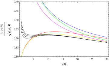
Figure 1: The circular velocity of a ball source of mass $M$ and radius $\mathcal{R}$, with the potentials of Table 1. We indicate case A by green line, case B by yellow line, case D by red line, case C by blue line, and the GR case by magenta line. The black line correspond to the Sanders model for $-0.95\,<\,\alpha\,<\,-0.92$. The values of free parameters are: $\omega(\phi^{(0)})\,=\,-1/2$, $\xi\,=\,-5$, $\eta\,=\,.3$, $m_{Y}\,=\,1.5*m_{R}$, $m_{S}\,=\,1.5*m_{R}$, $m_{R}\,=\,.1*\mathcal{R}^{-1}$

IV.2 Rotating sources and orbital parameters

Considering the geodesic equations (77) with the Christoffel symbols given in Eq. (IV), we obtain

$$\frac{d^{2}x^{i}}{ds^{2}}+\Gamma^{i}_{tt}+2\Gamma^{i}_{tj}\frac{dx^{j}}{ds}\,=\,0~{},$$ (82)

which in the coordinate system ${\bf J}\,=\,(0,0,J)$, reads

$$\ddot{x}+\frac{GM}{r^{3}}x\,=\,-\frac{GM\Lambda(r)}{r^{3}}x+\frac{2GJ}{r^{5}}\biggl{\{}\zeta(r)\biggl{[}\biggl{(}x^{2}+y^{2}-2z^{2}\biggl{)}\dot{y}+3yz\dot{z}\biggr{]}+2\Sigma(r)L_{x}z\biggr{\}}~{},$$

$$\ddot{y}+\frac{GM}{r^{3}}y\,=\,-\frac{GM\Lambda(r)}{r^{3}}y-\frac{2GJ}{r^{5}}\biggl{\{}\zeta(r)\biggl{[}\biggl{(}x^{2}+y^{2}-2z^{2}\biggl{)}\dot{x}+3xz\dot{z}\biggl{]}-2\Sigma(r)L_{y}z\biggr{\}}~{},$$ (83)

$$\ddot{z}+\frac{GM}{r^{3}}z\,=\,-\frac{GM\Lambda(r)}{r^{3}}z+\frac{6GJ}{r^{5}}\biggl{\{}\zeta(r)+\frac{2}{3}\Sigma(r)\biggr{\}}L_{z}z~{},$$

where

$$\Lambda(r)\,\doteq\,g(\xi,\eta)\,F(m_{R}\tilde{k}_{R}\mathcal{R})\,(1+m_{R}\tilde{k}_{R}r)\,e^{-m_{R}\tilde{k}_{R}r}+[1/3-g(\xi,\eta)]\,F(m_{R}\tilde{k}_{\phi}\mathcal{R})\,(1+m_{R}\tilde{k}_{\phi}r)\,e^{-m_{R}\tilde{k}_{\phi}r}$$

$$\qquad\qquad-\frac{4\,F(m_{Y}\mathcal{R})}{3}\,(1+m_{Y}r)\,e^{-m_{Y}r}~{},$$

$$\zeta(r)\,\doteq\,1-\bigl{[}1+m_{Y}r+(m_{Y}r)^{2}\bigr{]}e^{-m_{Y}r}~{},$$ (84)

$$\Sigma(r)\,\doteq\,(m_{Y}r)^{2}e^{-m_{Y}r}\,~{},$$

with $L_{x}$,$L_{y}$ and $L_{z}$ the components of the angular momentum.

The first terms in the right-hand-side of Eq. (IV.2), depending on the three parameters $m_{R},m_{Y}$ and $m_{\phi}$, represent the Extended Gravity (EG) modification of the Newtonian acceleration. The second terms in these equations, depending on the angular momentum $J$ and the EG parameters $m_{R},m_{Y}$ and $m_{\phi}$, correspond to dragging contributions. The case $m_{R}\rightarrow\infty,\,m_{Y}\rightarrow\infty$ and $m_{\phi}\rightarrow 0$ leads to $\Lambda(r)\rightarrow 0$, $\zeta(r)\rightarrow 1$ and $\Sigma(r)\rightarrow 0$, and hence one recovers the familiar results of GR  LenseThirring . These additional gravitational terms can be considered as perturbations of Newtonian gravity, and their effects on planetary motions can be calculated within the usual perturbative schemes assuming the Gauss equations RoyOrbit . We will follow this approach in what follows.

Let us consider the right-hand-side of Eq. (IV.2) as the components $(A_{x},A_{y},A_{z})$ of the perturbing acceleration in the system ($X,Y,Z$) (see Fig. 2), with $X$ the axis passing through the vernal equinox $\gamma$, $Y$ the transversal axis, and $Z$ the orthogonal axis parallel to the angular momentum J of the central body. In the system ($S,T,W$), the three components can be expressed as $(A_{s},A_{t},A_{w})$, with $S$ the radial axis, $T$ the transversal axis, and $W$ the orthogonal one. We will adopt the standard notation: $a$ is the semimajor axis; $e$ is the eccentricity; $p=a(1-e^{2})$ is the semilatus rectum; $i$ is the inclination; $\Omega$ is the longitude of the ascending node $N$; $\tilde{\omega}$ is the longitude of the pericenter $\Pi$; $M^{0}$ is the longitude of the satellite at time $t=0$; $\nu$ is the true anomaly; $u$ is the argument of the latitude given by $u=\nu+\tilde{\omega}-\Omega$; $n$ is the mean daily motion equal to $n=(GM/a^{3})^{1/2}$; and $C$ is twice the velocity, namely $C=r^{2}\dot{\nu}a^{2}(1-e^{2})^{1/2}$.

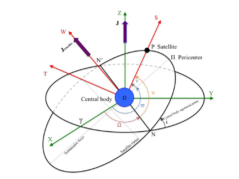
Figure 2: $i$ =  $)<$ $YN\Pi$ is the inclination; $\Omega$ =  $)<$ $XON$ is the longitude of the ascending node $N$; $\tilde{\omega}$= broken $)<$ $XO\Pi$ is the longitude of the pericenter $\Pi$; $\nu$ =  $)<$ $\Pi OP$ is the true anomaly; $u$ =  $)<$ $\Omega OP$=$\nu+\tilde{\omega}-\Omega$ is the argument of the latitude; J is the angular momentum of rotation of the central body; and $\textbf{J}_{\rm Satellite}$ is the angular momentum of revolution of a satellite around the central body.

The transformation rules between the coordinates frames ($X,Y,Z$) and ($S,T,W$) are

$$\begin{array}[]{ll}x\,=\,r(\cos u\cos\Omega-\sin u\sin\Omega\cos i)~{},\\ y\,=\,r(\cos u\sin\Omega+\sin u\cos\Omega\cos i)~{},\\ z\,=\,r\sin u\sin i\\ r\,=\,\frac{p}{1+e\cos\nu}~{},\end{array}$$ (89)

and the components of the angular momentum obey the equations

$$L_{x}\,=\,y\dot{z}-z\dot{y}=C\sin i\,\sin\Omega~{},$$

$$L_{y}\,=\,z\dot{x}-x\dot{z}=-C\cos\Omega\,\sin i~{},$$ (90)

$$L_{z}\,=\,x\dot{y}-y\dot{x}=C\cos i~{}.$$

The components of the perturbing acceleration in the ($S,\,T,\,W$) system read

$$A_{s}\,=\,-\frac{G\,M\,\Lambda(r)}{r^{2}}+\frac{2\,G\,J\,C\cos i}{r^{4}}\zeta(r)~{},$$

$$A_{t}\,=\,-\frac{2\,G\,J\,C\,e\cos\,i\sin\nu}{p\,r^{3}}\zeta(r)~{},$$ (91)

$$A_{w}\,=\,\frac{2\,G\,J\,C\sin i}{r^{4}}\left[\left(\frac{r\,e\sin\nu\cos u}{p}+2\sin u\right)\zeta(r)+2\sin u\,\Sigma(r)\right]~{}.$$

The $A_{s}$ component has two contributions: the former one results from the modified Newtonian potential $\Phi_{\rm ball}(\mathbf{x})$, while the latter one results from the gravito-magnetic field $A_{i}$ and it is a higher order term than the first one. Note that the components $A_{t}$ and $A_{w}$ depend only on the gravito-magnetic field. The Gauss equations for the variations of the six orbital parameters, resulting from the perturbing acceleration with components $A_{x},A_{y},A_{z}$, read

$$\begin{array}[]{ll}\frac{da}{dt}\,=\,\dot{a}_{\rm EG}\,=\,\frac{2e\,G\,M\,\Lambda(r)\,\sin\nu}{n\,\,\sqrt[]{1-e^{2}}\,C}\dot{\nu}~{},\\ \frac{de}{dt}\,=\,\dot{e}_{\rm GR}+\dot{e}_{\rm EG}\,=\,\frac{\sqrt[]{1-e^{2}}\,G\,M\,\Lambda(r)\,\sin\nu}{n\,a\,C}\dot{\nu}+\dot{e}_{\rm GR}\biggl{[}1-\,e^{-m_{Y}r}\Bigl{(}1+m_{Y}r+(m_{Y}r)^{2}\Bigr{)}\biggl{]}~{},\\ \frac{d\Omega}{dt}\,=\,\dot{\Omega}_{\rm GR}+\dot{\Omega}_{\rm EG}\,=\,\dot{\Omega}_{\rm GR}\biggl{\{}1-\,e^{-m_{Y}r}\Bigl{[}1+m_{Y}r+\bigl{(}1+f(\nu,u,e)\bigl{)}(m_{Y}r)^{2}\Bigl{]}\biggl{\}}~{},\\ \frac{di}{dt}\,=\,\dot{i}_{\rm GR}+\dot{i}_{\rm EG}\,=\,\dot{i}_{\rm GR}\biggl{\{}1-\,e^{-m_{Y}r}\Bigl{[}1+m_{Y}r+\bigl{(}1+f(\nu,u,e)\bigl{)}(m_{Y}r)^{2}\Bigl{]}\biggl{\}}~{},\\ \frac{d\tilde{\omega}}{dt}\,=\,\dot{\tilde{\omega}}_{\rm GR}+\dot{\tilde{\omega}}_{\rm EG}\,=\,-\frac{\sqrt[]{1-e^{2}}\,G\,M\,\Lambda(r)\,\cos\nu}{n\,a\,e\,C}\dot{\nu}+\dot{\tilde{\omega}}_{\rm GR}\biggl{[}1-\,e^{-m_{Y}r}\Bigl{(}1+m_{Y}r+(m_{Y}r)^{2}\Bigr{)}\biggl{]}\\ \qquad\qquad\qquad\qquad\qquad\qquad\qquad\qquad\qquad\qquad\qquad\qquad\qquad-2\sin^{2}\frac{i}{2}\,\dot{\Omega}_{\rm GR}f(\nu,u,e)\Sigma(r)~{},\\ \frac{dM^{0}}{dt}\,=\,\dot{M^{0}}_{\rm GR}+\dot{M^{0}}_{\rm EG}\,=\,-\frac{G\,M\,\Lambda(r)}{n\,a\,C}\biggl{[}\frac{2r}{a}+\frac{e\,\,\,\sqrt[]{1-e^{2}}}{1+\,\,\sqrt[]{1-e^{2}}}\cos\nu\biggl{]}\dot{\nu}+\dot{M^{0}}_{\rm GR}\biggl{[}1-\,e^{-m_{Y}r}\Bigl{(}1+m_{Y}r+(m_{Y}r)^{2}\Bigr{)}\biggl{]}\\ \qquad\qquad\qquad\qquad\qquad\qquad\qquad\qquad\qquad\qquad\qquad\qquad\qquad\qquad\qquad\qquad\qquad-2\sin^{2}\frac{i}{2}\,\dot{\Omega}_{\rm GR}f(\nu,u,e)\Sigma(r)~{},\end{array}$$ (100)

where

$$\begin{array}[]{ll}\dot{e}_{\rm GR}\,=\,\frac{2\,G\,J\cos i\sin\nu}{a\,C}\dot{\nu}~{},\\ \dot{\Omega}_{\rm GR}\,=\,\frac{2\,G\,J\sin u}{p\,C}\biggl{[}e\sin\nu\cos u+2\biggl{(}1+e\cos\nu\biggl{)}\sin u\biggl{]}\dot{\nu}~{},\\ \dot{i}_{\rm GR}\,=\,\frac{2\,G\,J\cos u\sin i}{C\,p}\biggl{[}e\sin\nu\cos u+2\biggl{(}1+e\cos\nu\biggl{)}\sin u\biggl{]}\dot{\nu}~{},\\ \dot{\tilde{\omega}}_{\rm GR}\,=\,-\frac{2\,G\,J\cos i}{a\,C}\left(2+\frac{1+e^{2}}{e}\cos\nu\right)\dot{\nu}+2\sin^{2}\frac{i}{2}\,\dot{\Omega}_{\rm GR}~{},\\ \dot{{\cal M}^{0}}_{\rm GR}\,=\,-\frac{4\,G\,J\cos i}{n\,a^{2}\,p}\biggl{(}1+e\cos\nu\biggl{)}\dot{\nu}+\frac{e^{2}}{1+\,\,\sqrt[]{1-e^{2}}}\dot{\tilde{\omega}}_{\rm GR}+2\,\,\sqrt[]{1-e^{2}}\sin^{2}\frac{i}{2}\,\dot{\Omega}_{\rm GR}~{},\\ f(\nu,u,e)\,=\,\frac{1+e\cos\nu}{1+e\left(\frac{\sin\nu\cot u}{2}+\cos\nu\right)}~{}.\end{array}$$ (107)

Hence, we have derived the corresponding equations of the six orbital parameters for Extended Gravity, with the dynamics of $a,e,\tilde{\omega},L^{0}$ depending mainly on the terms related to the modifications of the Newtonian potential, whilst the dynamics of $\Omega$ and $i$ depending only on the dragging terms.

Considering an almost circular orbit ($e\ll 1$), we integrate the Gauss equations with respect to the only anomaly $\nu$, from $0$ to $\nu(t)\,=\,nt$, since all other parameters have a slower evolution than $\nu$, hence they can be considered as constraints with respect to $\nu$. At first order we get

$$\begin{array}[]{ll}\Delta a(t)\,=\,0~{},\\ \Delta e(t)\,=\,0~{},\\ \Delta i(t)\,=\,\frac{G\,J\,e^{2}\,\sin i}{na^{3}}e^{-m_{Y}p}(m_{Y}p)^{2}\biggl{[}1+\frac{(m_{Y}p)^{2}}{2}\biggl{(}m_{Y}p-4\biggl{)}\biggl{]}\sin\biggl{(}\tilde{\omega}(t)-\Omega(t)\biggl{)}\nu(t)+{\cal O}(e^{4})~{},\\ \Delta\Omega(t)\,=\,\frac{2\,G\,J}{na^{3}}\biggl{[}1-e^{-m_{Y}p}\biggl{(}1+m_{Y}p+2(m_{Y}p)^{2}\biggl{)}\biggl{]}\nu(t)+{\cal O}(e^{2})~{},\\ \Delta\tilde{\omega}(t)\,=\,\biggl{\{}\frac{\tilde{\Lambda}(p)}{2}-\frac{2\,G\,J}{na^{3}}\biggl{[}3\cos i-1+e^{-m_{Y}p}(1+m_{Y}p+\frac{3}{2}(m_{Y}p)^{2}\\ \qquad\qquad\qquad\qquad\qquad\qquad-(3+3m_{Y}p+3(m_{Y}p)^{2}+\frac{1}{12}(m_{Y}p)^{3})\cos i)\biggl{]}\biggr{\}}\nu(t)+{\cal O}(e^{2})~{},\\ \Delta{\cal M}^{0}(t)\,=\,\biggl{\{}2\Lambda(p)-\frac{2\,G\,J}{na^{3}}\biggl{[}3\cos i-1-e^{-m_{Y}p}\biggl{(}1+m_{Y}p+2(m_{Y}p)^{2}\biggl{)}\biggl{(}\cos i-1\biggl{)}\biggl{]}\biggr{\}}\nu(t)+{\cal O}(e^{2})~{},\end{array}$$ (115)

where

$$\tilde{\Lambda}(p) \doteq g(\xi,\eta)\,F(m_{R}\tilde{k}_{R}\mathcal{R})\,(m_{R}\tilde{k}_{R}p)^{2}\,e^{-m_{R}\tilde{k}_{R}p}+[1/3-g(\xi,\eta)]\,F(m_{R}\tilde{k}_{\phi}\mathcal{R})\,(m_{R}\tilde{k}_{\phi}p)^{2}\,e^{-m_{R}\tilde{k}_{\phi}p}$$

$$-\frac{4\,F(m_{Y}\mathcal{R})}{3}\,(m_{Y}p)^{2}\,e^{-m_{Y}p}~{}.$$

We hence notice that the contributions to the semimajor axis $a$ and eccentricity $e$ vanish, as in GR, whilst there are nonzero contributions to $i$, $\Omega$, $\tilde{\omega}$ and $M^{0}$. In particular, the contributions to the inclination $i$ and the longitude of the ascending node $\Omega$, depend only on the drag effects of the rotating central body; while the contributions to the pericenter longitude $\tilde{\omega}$ and mean longitude at $M^{0}$, depend also on the modified Newtonian potential. Finally, note that in the Extended Gravity model we have considered here, the inclination $i$ has a nonzero contribution, in contrast to the result obtained within GR, and also $\Delta\tilde{\omega}(t)\neq\Delta M^{0}(t)$, given by

$$\Delta\tilde{\omega}(t)-\Delta{\cal M}^{0}(t)\simeq \biggl{\{}\frac{\tilde{\Lambda}(p)-4\Lambda(p)}{2}+\frac{2GJ}{na^{3}}e^{-m_{Y}p}\biggl{[}\frac{(m_{Y}p)^{2}}{2}+(2+2m_{Y}p+(m_{Y}p)^{2}$$

$$\qquad+\frac{(m_{Y}p)^{3}}{12})\cos i\biggr{]}\biggl{\}}\,\nu(t)+{\cal O}(e^{2})~{}.$$

In the limit $m_{R}\rightarrow\infty,m_{Y}\rightarrow\infty$ and $m_{\phi}\rightarrow 0$, we obtain the well-known results of GR.

V Experimental constraints

The orbiting gyroscope precession can be split into a part generated by the metric potentials, $\Phi$ and $\Psi$, and one generated by the vector potential $\mathbf{A}$. The equation of motion for the gyro-spin three-vector $\mathbf{S}$ is

$$\frac{d\mathbf{S}}{dt}\,=\,\frac{d\mathbf{S}}{dt}\Big{|}_{\text{G}}+\frac{d\mathbf{S}}{dt}\Big{|}_{\text{LT}}$$ (118)

where the geodesic and Lense-Thirring precessions are

$$\frac{d\mathbf{S}}{dt}\Big{|}_{\text{G}}\,=\,\mathbf{\Omega}_{\text{G}}\times\mathbf{S}\,\,\,\,\text{with}\,\,\,\,\mathbf{\Omega}_{\text{G}}\,=\,\frac{\nabla(\Phi+2\Psi)}{2}\times\mathbf{v}~{},$$

(119)

$$\frac{d\mathbf{S}}{dt}\Big{|}_{\text{LT}}\,=\,\mathbf{\Omega}_{\text{LT}}\times\mathbf{S}\,\,\,\,\text{with}\,\,\,\,\mathbf{\Omega}_{\text{LT}}\,=\,\frac{\nabla\times\mathbf{A}}{2}~{}.$$

The geodesic precession, $\mathbf{\Omega}_{G}$, can be written as the sum of two terms, one obtained with GR and the other being the Extended Gravity contribution. Then we have

$$\mathbf{\Omega}_{\text{G}}\,=\,\mathbf{\Omega}_{\text{G}}^{\text{(GR)}}+\mathbf{\Omega}_{\text{G}}^{\text{(EG)}}~{},$$ (120)

where

$$\mathbf{\Omega}_{\text{G}}^{\text{(GR)}}\,=\,\frac{3GM}{2|\mathbf{x}|^{3}}\,\,\mathbf{x}\times\mathbf{v}~{},$$

$$\mathbf{\Omega}_{\text{G}}^{\text{(EG)}}\,=\,-\biggl{[}g(\xi,\eta)(m_{R}\tilde{k}_{R}r+1)\,F(m_{R}\tilde{k}_{R}\mathcal{R})\,e^{-m_{R}\tilde{k}_{R}r}+\frac{8}{3}(m_{Y}r+1)\,F(m_{Y}\mathcal{R})\,e^{-m_{Y}r}$$ (121)

$$\qquad\qquad\qquad\qquad\qquad\qquad\qquad\qquad+\biggl{[}\frac{1}{3}-g(\xi,\eta)](m_{R}\tilde{k}_{\phi}r+1)F(m_{R}\tilde{k}_{\phi}\mathcal{R})\,e^{-m_{R}\tilde{k}_{\phi}r}\biggr{]}\frac{{\bf\Omega}_{\rm G}^{\rm(GR)}}{3}~{}.$$

where $|\textbf{x}|=r$. Similarly one has

$$\mathbf{\Omega}_{\text{LT}}\,=\,\mathbf{\Omega}_{\text{LT}}^{\text{(GR)}}+\mathbf{\Omega}_{\text{LT}}^{\text{(EG)}}~{},$$ (122)

with

$$\mathbf{\Omega}_{\text{LT}}^{\text{(GR)}}\,=\,\frac{G}{2r^{3}}\,\mathbf{J}~{},$$

(123)

$$\mathbf{\Omega}_{\text{LT}}^{\text{(EG)}}\,=\,-e^{-m_{Y}r}(1+m_{Y}r+{m_{Y}}^{2}r^{2})\,\mathbf{\Omega}_{\text{LT}}^{\text{(GR)}}~{},$$

where we have assumed that, on the average, $\langle(\mathbf{J}\cdot\mathbf{x})\,\mathbf{x}\rangle\,=\,0$.

Gravity Probe B satellite contains a set of four gyroscopes and has tested two predictions of GR: the geodetic effect and frame-dragging (Lense-Thirring effect). The tiny changes in the direction of spin gyroscopes, contained in the satellite orbiting at $h=650$ km of altitude and crossing directly over the poles, have been measured with extreme precision. The values of the geodesic precession and the Lense-Thirring precession, measured by the Gravity Probe B satellite and those predicted by GR, are given in Table II.

Table 2: The geodesic precession and Lense-Thitting (frame dragging) precession as predicted by GR and observed with the Gravity Probe B experiment GPBexp .

Effect	Measured (mas/y)	Predicted (mas/y)
Geodesic precession	$6602\pm 18$	6606
Lense-Thirring precession	$\ \ \ \ \ \ 37.2\pm 7.2$	39.2

Imposing the constraint $|\mathbf{\Omega}_{\text{G}}^{\text{(EG)}}|\,\lesssim\,\delta\mathbf{\Omega}_{\text{G}}$ and $|\mathbf{\Omega}_{\text{LT}}^{\text{(EG)}}|\,\lesssim\,\delta\mathbf{\Omega}_{\text{LT}}$, LamSakSta , with $r^{*}\,=\,R_{\oplus}+h$ where $R_{\oplus}$ is the radius of the Earth and $h\,=\,650\,km$ is the altitude of the satellite, we get

$$g(\xi,\eta)\big{(}m_{R}\tilde{k}_{R}\,r^{*}+1)\,F(m_{R}\tilde{k}_{R}R_{\oplus})\,e^{-m_{R}\tilde{k}_{R}\,r^{*}}+[1/3-g(\xi,\eta)](m_{R}\tilde{k}_{\phi}\,r^{*}+1)\,F(m_{R}\tilde{k}_{\phi}R_{\oplus})\,e^{-m_{R}\tilde{k}_{\phi}\,r^{*}}$$

$$\qquad\qquad\qquad\qquad\qquad\qquad\qquad\qquad\qquad+\frac{8}{3}(m_{Y}\,r^{*}+1)\,F(m_{Y}R_{\oplus})\,e^{-m_{Y}\,r^{*}}\,\lesssim\,\frac{3\,\delta|\mathbf{\Omega}_{\text{G}}|}{|\mathbf{\Omega}_{\text{G}}^{\text{(GR)}}|}\simeq 0.008~{},$$ (124)

$$(1+m_{Y}r^{*}+{m_{Y}}^{2}{r^{*}}^{2})\,e^{-m_{Y}r^{*}}\,\lesssim\,\frac{\,\delta|\mathbf{\Omega}_{\text{LT}}|}{|\mathbf{\Omega}_{\text{LT}}^{\text{(GR)}}|}\simeq 0.19~{},$$

since, from the experiments, we have $|\mathbf{\Omega}_{\text{G}}^{\text{(GR)}}|\,=\,6606\,{\rm mas}$ and $\delta|\mathbf{\Omega}_{\text{G}}|\,=\,18\,{\rm mas}$, $|\mathbf{\Omega}_{\text{LT}}^{\text{(GR)}}|\,=\,37.2\,{\rm mas}$ and $\delta|\mathbf{\Omega}_{\text{LT}}|\,=\,7.2\,{\rm mas}$. From Eq. (V) we thus obtain that $m_{Y}\geq 7.3\times 10^{-7}m^{-1}$.

The LAser RElativity Satellite (LARES) mission laresdata of the Italian Space Agency is designed to test the frame-dragging and the Lense-Thirring effect, to within 1$\%$ of the value predicted in the framework of GR. The body of this satellite has a diameter of about 36.4 cm and weights about 400 kg. It was inserted in an orbit with 1450 km of perigee, an inclination of $69.5\pm 1$ degrees and eccentricity $9.54\times 10^{-4}$. It allows us to obtain a stronger constraint for $m_{Y}$:

$$(1+m_{Y}r^{*}+{m_{Y}}^{2}{r^{*}}^{2})\,e^{-m_{Y}r^{*}}\,\lesssim\,\frac{\,\delta|\mathbf{\Omega}_{\text{LT}}|}{|\mathbf{\Omega}_{\text{LT}}^{\text{(GR)}}|}\simeq 0.01~{},$$ (125)

from the which we obtain $m_{Y}\geq 1.2\times 10^{-6}m^{-1}$.

In the specific case of the Noncommutative Spectral Geometry model, the quantities (28) become $m_{R}\rightarrow\infty$, $m_{Y}=\sqrt{\frac{5\pi^{2}\bigl{(}k_{0}^{2}{\bf H}^{(0)}-6\bigr{)}}{36f_{0}k_{0}^{2}}}$ and $m_{\phi}=0$, implying that $\xi=\frac{af_{0}({\bf H}^{(0)})^{2}}{12\pi^{2}}$, $\eta=0$ , $g(\xi,\eta)=\frac{af_{0}({\bf H}^{(0)})^{2}+12\pi^{2}}{6|af_{0}({\bf H}^{(0)})^{2}-12\pi^{2}|}+\frac{1}{6}$ and ${\tilde{k}_{R,\phi}}^{2}=1-\frac{af_{0}({\bf H}^{(0)})^{2}}{12\pi^{2}}\,,\,0$. The first relation (V) becomes

$$\frac{8}{3}(m_{Y}\,r^{*}+1)\,F(m_{Y}R_{\oplus})\,e^{-m_{Y}\,r^{*}}\,\lesssim\,0.008~{},$$

hence the constraint on $m_{Y}$ imposed from GBP is

$$m_{Y}>7.1\times 10^{-5}{\rm m}^{-1}~{},$$

whereas the LARES experiment (125) implies

$$m_{Y}>1.2\times 10^{-6}{\rm m}^{-1}~{},$$

a bound similar to the one obtained earlier on using binary pulsars Nelson:2010ru , or the Gravity Probe B data LamSakSta . It is important to note that a much stronger limit, $m_{Y}>10^{4}{\rm m}^{-1}$, has been obtained using the torsion balance experiments LamSakSta .

In conclusion, using data form Gravity Probe B and LARES missions, we obtain similar constraints on $m_{Y}$; a result that one could have anticipated since both these experiments are designed to test the same type of physical phenomenon. However, by using the stronger constraint for $m_{Y},$ namely $m_{Y}>10^{4}{\rm m}^{-1}$, we observe that the modifications to the orbital parameters (100) induced by Noncommutative Spectral Geometry are indeed small, confirming the consistency between the predictions of NCSG as a gravitational theory beyond GR and the Gravity Probe B and LARES measurements. At this point let us stress that, in principle, space-based experiments can be used to test parameters of fundamental theories.

VI Conclusions

In the context of Extended Gravity, we have studied the linearized field equations in the limit of weak gravitational fields and small velocities generated by rotating gravitational sources, aiming at constraining the free parameters, which can be seen as effectives masses (or lengths), using recent recent experimental results. We have studied the precession of spin of a gyroscope orbiting about a rotating gravitational source. Such a gravitational field gives rise, according to GR predictions, to geodesic and Lense-Thirring processions, the latter being strictly related to the off-diagonal terms of the metric tensor generated by the rotation of the source. We have focused in particular on the gravitational field generated by the Earth, and on the recent experimental results obtained by the Gravity Probe B satellite, which tested the geodesic and Lense-Thirring spin precessions with high precision.

In particular, we have calculated the corrections of the precession induced by scalar, tensor and curvature corrections. Considering an almost circular orbit, we integrated the Gauss equations and obtained the variation of the parameters at first order with respect to the eccentricity. We have shown that the induced EG effects depend on the effective masses $m_{R}$, $m_{Y}$ and $m_{\phi}$ (115), while the nonvalidity of the Gauss theorem implies that these effects also depend on the geometric form and size of the rotating source. Requiring that the corrections are within the experimental errors, we then imposed constraints on the free parameters of the considered EG model. Merging the experimental results of Gravity Probe B and LARES, our results can be summarized as follows:

$$g(\xi,\eta)\big{(}m_{R}\tilde{k}_{R}\,r^{*}+1)\,F(m_{R}\tilde{k}_{R}R_{\oplus})\,e^{-m_{R}\tilde{k}_{R}\,r^{*}}+[1/3-g(\xi,\eta)](m_{R}\tilde{k}_{\phi}\,r^{*}+1)\,F(m_{R}\tilde{k}_{\phi}R_{\oplus})\,e^{-m_{R}\tilde{k}_{\phi}\,r^{*}}$$

$$\qquad\qquad\qquad\qquad\qquad\qquad\qquad\qquad\qquad+\frac{8}{3}(m_{Y}\,r^{*}+1)\,F(m_{Y}R_{\oplus})\,e^{-m_{Y}\,r^{*}}\,\lesssim\,0.008~{},$$ (126)

and

$$m_{Y}\geq 1.2\times 10^{-6}m^{-1}~{}.$$ (127)

It is interesting to note that the field equation for the potential $A_{i}$, Eq. (58c), is time-independent provided the potential $\Phi$ is time-independent. This aspect guarantees that the solution Eq. (76) does not depend on the masses $m_{R}$ and $m_{\phi}$ and, in the case of $f(R,\,\phi)$ gravity, the solution is the same as in GR. In the case of spherical symmetry, the hypothesis of a radially static source is no longer considered, and the obtained solutions depend on choice of the $f(R,\,\phi)$ ET model, since the geometric factor $F(x)$ is time-dependent. Hence in this case, gravito-magnetic corrections to GR emerge with time-dependent sources.

A final remark deserves the case of Noncommutative Spectral Geometry that we discussed above. This model descends from a fundamental theory and can be considered as a particular case of Extended Gravity. Its parameters, can be probed in the weak-field limit and at local scales, opening new perspectives worth to be further developed stequest ; GINGER .

References

• (1) Capozziello S., De Laurentis M., Phyisics Reports 509, 167 (2011).
• (2) Nojiri S., Odintsov S.D., Phys. Rept. 505, 59 (2011).
• (3) Nojiri S., Odintsov S.D., Int. J. Geom. Meth. Mod. Phys. 4, 115 (2007).
• (4) Capozziello S., Francaviglia M., Gen. Rel. Grav. 40,357, (2008).
• (5) Capozziello S., De Laurentis M., Faraoni V., The Open Astr. Jour 2, 1874 (2009).
• (6) Capozziello S., Faraoni V., Beyond Einstein gravity: A Survey of gravitational theories for cosmology and astrophysics, Fundamental Theories of Physics, Vol. 170, Springer, New York (2010).
• (7) Capozziello S., De Laurentis M., Invariance Principles and Extended Gravity: Theory and Probes, Nova Science Publishers, New York (2010).
• (8) Quandt I., Schmidt H.J., Astron. Nachr. 312, 97 (1991). Teyssandier P., Class. Quant. Grav. 6, 219 (1989). S. Capozziello, G. Lambiase, Int. J. Mod. Phys. D 12, 843 (2003). S. Calchi Novati, S. Capozziello, G. Lambiase, Grav. Cosmol. 6, 173 (2000).
• (9) Will C.M., Theory and Experiment in Gravitational Physics, 2nd ed. Cambridge University Press, Cambridge, UK (1993).
• (10) Capozziello S., De Laurentis M., Annalen Phys. 524, 545 (2012).
• (11) Altschul B, Bailey Q.G., et al. to appear in Advances in Space Research (2014) arXiv:1404.4307 [gr-qc].
• (12) Capozziello S., Stabile A. Class. Quant. Grav. 26, 085019 (2009).
• (13) A. Connes, Noncommutative Geometry, Academic Press, New York (1994)
• (14) A. Connes and M. Marcolli, Noncommutative Geometry, Quantum Fields and Motives, Hindustan Book Agency, India (2008)
• (15) A. H. Chamseddine and A. Connes, Commun. Math. Phys.  186 (1997) 731 [hep-th/9606001].
• (16) M. Sakellariadou, Int. J. Mod. Phys. D 20, 785 (2011) [arXiv:1008.5348 [hep-th]].
• (17) M. Sakellariadou,PoS CORFU 2011, 053 (2011) [arXiv:1204.5772 [hep-th]].
• (18) K. van den Dungen and W. D. van Suijlekom, Rev. Math. Phys.  24 (2012) 1230004 [arXiv:1204.0328 [hep-th]].
• (19) A. H. Chamseddine, A. Connes and M. Marcolli, Adv. Theor. Math. Phys.  11, 991 (2007) [arXiv:hep-th/0610241].
• (20) A. H. Chamseddine and A. Connes, JHEP 1209, 104 (2012) [arXiv:1208.1030 [hep-ph]].
• (21) A. H. Chamseddine and A. Connes, Phys. Rev. Lett.  99 (2007) 191601 [arXiv:0706.3690 [hep-th]].
• (22) M. Sakellariadou, A. Stabile and G. Vitiello, Phys. Rev. D 84, 045026 (2011) [arXiv:1106.4164 [math-ph]].
• (23) M. V. Gargiulo, M. Sakellariadou and G. Vitiello, [arXiv:1305.0659 [hep-th]].
• (24) A. Devastato, F. Lizzi and P. Martinetti, [arXiv:1304.0415 [hep-th]].
• (25) A. H. Chamseddine, A. Connes and W. D. van Suijlekom, arXiv:1304.8050 [hep-th].
• (26) A. H. Chamseddine and A. Connes, J. Math. Phys.  47 (2006) 063504 [hep-th/0512169].
• (27) A. H. Chamseddine and A. Connes, Commun. Math. Phys.  293 (2010) 867 [arXiv:0812.0165 [hep-th]].
• (28) W. Nelson and M. Sakellariadou, Phys. Rev. D 81, 085038 (2010) [arXiv:0812.1657 [hep-th]].
• (29) W. Nelson and M. Sakellariadou, Phys. Lett.  B 680, 263 (2009) [arXiv:0903.1520 [hep-th]].
• (30) M. Marcolli and E. Pierpaoli, Adv. Theor. Math. Phys.  14 (2010) [arXiv:0908.3683 [hep-th]].
• (31) M. Buck, M. Fairbairn and M. Sakellariadou, Phys. Rev. D 82, 043509 (2010) [arXiv:1005.1188 [hep-th]].
• (32) J. F. Donoghue, Phys. Rev. D 50 (1994) 3874 [gr-qc/9405057].
• (33) Capozziello S., Stabile A., Troisi A., Phys. Rev. D 76, 104019 (2007).
• (34) Stabile A., Phys. Rev. D 82, 064021 (2010).
• (35) Stabile A., Phys. Rev. D 82, 124026 (2010).
• (36) Stabile A., Capozziello S., Phys. Rev. D 87, 064002 (2013).
• (37) Stabile A., Stabile An., Phys. Rev. D 85, 044014 (2012).
• (38) Stabile A., Scelza G., Phys. Rev. D 84, 124023 (2011).
• (39) Sanders R. H., Astron. Astrophys. 136, L21 (1984).
• (40) M. Milgrom, Astrophys. J.  270 (1983) 365.
• (41) J. D. Bekenstein, Phys. Rev. D 70 (2004) 083509 [Erratum-ibid. D 71 (2005) 069901] [astro-ph/0403694].
• (42) I. Ferreras, M. Sakellariadou and M. F. Yusaf, Phys. Rev. Lett.  100 (2008) 031302 [arXiv:0709.3189 [astro-ph]].
• (43) N. E. Mavromatos, M. Sakellariadou and M. F. Yusaf, Phys. Rev. D 79 (2009) 081301 [arXiv:0901.3932 [astro-ph.GA]].
• (44) I. Ferreras, N. E. Mavromatos, M. Sakellariadou and M. F. Yusaf, Phys. Rev. D 80 (2009) 103506 [arXiv:0907.1463 [astro-ph.GA]].
• (45) I. Ferreras, N. E. Mavromatos, M. Sakellariadou and M. F. Yusaf, Phys. Rev. D 86 (2012) 083507 [arXiv:1205.4880 [astro-ph.CO]].
• (46) N. Mavromatos and M. Sakellariadou, Phys. Lett. B 652 (2007) 97 [hep-th/0703156 [HEP-TH]].
• (47) N. E. Mavromatos, M. Sakellariadou and M. F. Yusaf, JCAP 1303 (2013) 015 [arXiv:1211.1726 [hep-th]].
• (48) Napolitano N. R., Capozziello S., Romanowsky A. J., Capaccioli M., Tortora C., ApJ 748, 87 (2012).
• (49) Lense J., Thirring H., Phys. Z 19, 33 (1918)
• (50) Roy A.E., Orbital Motion, IOP Publishing, Bristol (2005)
• (51) Everitt C.W.F., et al., Phys.  Rev.  Lett. 106, 221101 (2011).
• (52) Lambiase G., Sakellariadou M., Stabile An., JCAP 12, 020 (2013).
• (53) http://www.asi.it/it/attivita/cosmologia/lares
• (54) W. Nelson, J. Ochoa and M. Sakellariadou, Phys. Rev. Lett.  105, 101602 (2010) [arXiv:1005.4279 [hep-th]].
• (55) Besides GP-B and LARES experiments, it should be also mentioned GINGER experiment gingerexp , which is an Earth based experiment that aims to evaluate the response to the gravitational field of a ring laser array. GINGER forthcoming data will therefore allow to determine independent constraints on the parameters characterzing theories that generalize GR (see e.g. ninfa ).
• (56) See for example http://www.df.unipi.it/ginger.
• (57) N. Radicella, G. Lambiase, L. Parisi, and G. Vilasi, arXiv:1408.1247 [gr-qc].