Interferometric Tests of Planckian Quantum Geometry Models

Abstract

The effect of Planck scale quantum geometrical effects on measurements with interferometers is estimated with standard physics, and with a variety of proposed extensions. It is shown that effects are negligible in standard field theory with canonically quantized gravity. Statistical noise levels are estimated in a variety of proposals for non-standard metric fluctuations, and these alternatives are constrained using upper bounds on stochastic metric fluctuations from LIGO. Idealized models of several interferometer system architectures are used to predict signal noise spectra in a quantum geometry that cannot be described by a fluctuating metric, in which position noise arises from holographic bounds on directional information. Predictions in this case are shown to be close to current and projected experimental bounds.

I introduction

It is often remarked that quantum gravity should lead to the creation and annihilation of high energy virtual particles that gravitationally alter spacetime to be “foamy” or “fuzzy” at the Planck scale. While various models mathematically suggest such nonclassicalityWheeler (1963); Hawking (1978); Hawking et al. (1980); Ashtekar et al. (1992); Ellis et al. (1992), it is unclear exactly how much the actual physical metric departs from the classical structure, particularly in systems much larger than the Planck length. In particular, it is not known how the effects of Planck scale fluctuations perturb the geodesic of a macroscopic experimental object.

Laser interferometry is a particularly good experimental tool to test theories of position, because it is the most precise measure of relative space-time position of massive bodies. The LIGO collaboration has previously published limits on the stochastic gravitational-wave background that correspond to a spectral density of noise below the Planck spectral density– that is, the formal experimental bound on variance in dimensionless strain per frequency interval is now less than the Planck time. Having crossed the Planck threshold in experimental technique, there is a need for better controlled theoretical predictions for the characteristics of Planckian spacetime noise as they actually appear in interterferometer data, and a more systematic application of the experimental constraints to model parameters. This paper presents a survey of candidate models of Planckian quantum geometry, and computes their effects using schematic theoretical models of interferometers that are sufficiently detailed and well characterized to provide useful constraints on new physics.

A straightforward Planck-scale change in position is impossible to measure experimentally. Moreover, we show below that metric perturbations that fluctuate only at a microscopic scale average out in macroscopic measurements and thus become practically unobservable in real experiments. However, a beam splitter suspended in an interferometer such as LIGO is in free fall (i.e. following a geodesic) in horizontal directions at frequencies much higher than 100Hz Weiss (1972); Adhikari (2014); The LIGO Scientific Collaboration (2009). Thus, the effects of certain types of spacetime noise can accumulate over time, enough for some types of deviations from geodesics to be observable in extensions of known physics.

We start by calculating, in standard field theory, measurable fluctuations in a macroscopic spacetime distance expected from vacuum fluctuations in graviton fields. This calculation confirms the conventional wisdom that in standard field theory, Planck scale effects stay at the Planck scale: they average out to create negligible departures from classical behavior on macroscopic scales.

We then proceed to survey a variety of phenomenological proposals, based on conjectures about macroscopic quantum properties of the space-time metric. These extensions of standard physics are still based on metric perturbations, so they can be compared directly with published bounds on metric fluctuations from gravitational wave backgrounds. We classify the scaling behavior of metric perturbation noise with respect to the length scales involved in the measurementAmelino-Camelia (1999); *AmelinoCamelia2000; Amelino-Camelia (2001a); *AmelinoCamelia2001a; Ng and van Dam (2000); Wu and Ford (2000); Campbell-Smith et al. (1999), and compare these with experimental data from LIGO. Among the alternative models surveyed, we find that they generally are either already convincingly ruled out by current data, or do not produce detectable effects.

An important exception lies in a class of models where Planckian geometrical degrees of freedom cannot be expressed as fluctuations of a metric, treated in the usual way as quantized amplitudes of modes that have a determinate classical spatial structure. It has been known that field modes within a classical background spacetime result in infrared paradoxes of states denser than black holesCohen et al. (1999). Macroscopic geometrical uncertainty in a different kind of model can be estimated from the holographic information content of gravitational systems, and from general symmetry principles Fischler and Susskind (1998); Bousso (1999a, b, 2002). Spatial information can be regarded as being carried by null waves subject to a Planck frequency cut-off or bandwidth limitHogan (2008a, b, 2009); Hogan and Jackson (2009). This hypothesis predicts directional spacetime uncertainty that does not average away in the same way as fluctuations in field theoryHogan (2012a, b, c); indeed by some measures, it grows with scale. It also allows nonlocal entanglement of position states of a kind not available within the local framework of quantum field theory, while preserving causal relationships.

In these information-bounded models, the spatial coherence of fluctuations depends differently on the causal structure of the space-time than in the case of gravitational waves, or in metric-based extension models. Interferometers far apart from each other display a coherent, correlated response to a low frequency stochastic gravitational wave background. This is true even for small interferometers, as long as their separation is not much larger than the measured wavelength (on the order of $10^{6}\textrm{m}$ for gravitational-wave detectors). By contrast, fluctuations from information bounds are only correlated if the two interferometers measure causally overlapping space-time regions. The response of interferometer systems depends differently on their architectures – the layout of the optical paths in space. The apparatus must be modeled to take these differences into account in making predictions for signal correlations.

In the later sections of this paper we compare predictions in this kind of model with experimental bounds from LIGO and GEO-600, as well as future tests with the Fermilab Holometer, a pair of co-located, cross-correlated interferometers specifically designed to search for such effects. Since these perturbations are not equivalent to metric fluctuations, we develop models of the interferometers to estimate their response to this kind of geometrical uncertainty. We find that this class of model is close to being either ruled out or experimentally detectable.

Throughout this paper, where numerical values are needed, we use $\hbar=6.58\times 10^{-22}\textrm{ MeV s}$, $G=6.71\times 10^{-39}\textrm{ }\hbar c\textrm{ }(\textrm{GeV}/c^{2})^{-2}$, and $c=299792458\textrm{ m/s}$ K. A. Olive et al. (2014) (Particle Data Group).

II Constraints on Planckian Noise from Metric Fluctuations

II.1 Standard Field Theory

It is well-known that standard methods of quantizing general relativity as graviton fields lead to results that are not renormalizable. However, on macroscopic scales graviton self-interactions can be neglected, and it is consistent to use the zero-point amplitude of metric fluctuations to estimate the order of magnitude of metric fluctuations predicted by a model based on field theory.

Assume plane wave solutions in linearized gravity, and consider a wave incident perpendicular to a length being measured (e.g. an interferometer arm). The mean amplitude of a perturbation vanishes, but a graviton mode has a typical fluctuation energy on the order of $\frac{1}{2}\hbar\omega_{g}$, where $\omega_{g}$ is the frequency of the mode. Divided by the typical scale of volume that such a field would occupy, this corresponds to an energy density of:

$$u=\frac{\frac{1}{2}\hbar\omega_{g}}{(c/\omega_{g})^{3}}$$ (1)

A gravitational wave of strain amplitude $h$ has an energy density of:

$$u=\frac{c^{2}}{32\pi G}\omega_{g}^{2}h^{2}$$ (2)

Equating the two equations gives us a typical strain amplitude of:

$$h\approx 4\sqrt{\pi}\frac{l_{p}\omega_{g}}{c}$$ (3)

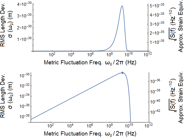
Figure 1: RMS length deviation in a $1\mu\textrm{m}$ laser beam extended over a 4km macroscopic distance, measured with two macroscopic boundary surfaces and generated by an optimally oriented graviton vacuum mode of zero-point energy $\frac{1}{2}\hbar\omega_{g}$. The result is also shown in equivalent strain, calculated by assuming a perfect detector response. This is not the same as strain noise observed in interferometers, as discussed below. Averaging the metric fluctuation over the minimum laser beam width causes exponential suppression at frequencies higher than $\omega_{g}=c\sqrt{2\pi/\mathcal{L}\lambda}$, the inverse diffraction scale. The value of the peak, marked above at 2GHz, is $4\times 10^{-30}\textrm{m}$ or $5\times 10^{-35}\textrm{Hz}^{-\frac{1}{2}}$.

If a gravitational plane wave of this strain amplitude travels in the $z$ direction, in a length $\mathcal{L}$ orthogonal to the propagation we expect a position fluctuation of the following time-dependent magnitude:

$$\Delta\mathcal{L}=F(z-ct) \equiv\frac{1}{2}\mathcal{L}h\cos(kz-\omega_{g}t)$$ (4)

$$=2\sqrt{\pi}\mathcal{L}\frac{l_{p}\omega_{g}}{c}\cos(\frac{\omega_{g}}{c}z-\omega_{g}t)$$ (5)

However, this is not the actual length fluctuation measurable between two macroscopic objects (e.g. mirrors). To determine the position of a macroscopic object, we need the object to interact with a measurable field, which occurs over a nonzero area. If we consider a light beam of wavelength $\lambda$ extended over a length $\mathcal{L}$, that would require the beam to have a minimum cross section width on the order of the diffraction scale, $\sqrt{\mathcal{L}\lambda/2\pi}$. The function $F(z-ct)$ varies with $z$ at a distance scale of $\frac{2\pi c}{\omega_{g}}$, which is much smaller than $\sqrt{\mathcal{L}\lambda/2\pi}$ for the higher-energy modes that lead to larger metric strain. Therefore the interaction between the surface of the object and the light beam would cause a significant amount of suppression in the measurable length fluctuation as we average across a macroscopic boundary of this width.

Now model the cross section of the beam as a gaussian. A one-dimensional averaging in the direction of an optimally oriented gravitational plane wave mode will suffice as a demonstrative example.

$$G(z)\equiv\frac{1}{\sqrt{\mathcal{L}\lambda}}\textrm{e}^{-\frac{\pi z^{2}}{\mathcal{L}\lambda}}$$ (6)

To find the measurable time-dependent fluctuation in $\mathcal{L}$, we average the fluctuation $F(z-ct)$ over the cross section of the beam by taking the following convolution with $G(z)$:

$$x(t) = \intop_{-\infty}^{\infty}F(z-ct)G(z)\textrm{d}z$$ (7)

$$= 2\sqrt{\pi}\frac{\mathcal{L}l_{p}\omega_{g}}{c}\cos(\omega_{g}t)\textrm{e}^{-\frac{\mathcal{L}\lambda\omega_{g}^{2}}{4\pi c^{2}}}$$ (8)

Take the RMS value over time:

$$\sigma(\omega_{g})=\sqrt{2\pi}\frac{\mathcal{L}l_{p}\omega_{g}}{c}\textrm{e}^{-\frac{\mathcal{L}\lambda\omega_{g}^{2}}{4\pi c^{2}}}$$ (9)

Figure 1 shows a plot of $\sigma(\omega_{g})$, assuming $\lambda=1\mu\textrm{m}$ and $\mathcal{L}=4\textrm{km}$ to match the physical parameters of LIGO, currently the most sensitive experiment for detecting such metric strains. As intuitively expected, higher frequency modes lead to higher zero-point energy and larger metric strain, but averaging the fluctuation over the beam width exponentially suppresses the observable macroscopic length deviation for those short-wavelength graviton modes. The resultant peak occurs at:

$$\omega_{g,\,max}=c\sqrt{\frac{2\pi}{\mathcal{L}\lambda}}\qquad\sigma(\omega_{g,\,max})=2\pi l_{p}\sqrt{\frac{\mathcal{L}}{\textrm{e}\lambda}}$$ (10)

The plot has a peak value of $4\times 10^{-30}\textrm{m}$ at 2GHz. This is clearly too small to be observed, and occurs at a frequency many orders of magnitude higher than the optimal measurement band for LIGO, which causes the detectable effect to be even further suppressed.

We sum over all frequency modes to obtain the total length fluctuation. Since the relevant length scale here is $\sqrt{\mathcal{L}\lambda/2\pi}$, we perform a dimensionless mode summation assuming a 1-dimensional box of that size. We apply the substitution:

$$\omega_{g}=2\pi f_{g}=\pi c\sqrt{\frac{2\pi}{\mathcal{L}\lambda}}n$$ (11)

and sum over values of n running from 0 to $\infty$. Since these are independent modes, to obtain the overall uncertainty in $\mathcal{L}$, we sum their contributions in quadrature:

$$\sigma_{tot} = \left[\int_{0}^{\infty}\left(\sqrt{2\pi}\frac{\mathcal{L}l_{p}}{c}\pi c\sqrt{\frac{2\pi}{\mathcal{L}\lambda}}n\textrm{e}^{-\frac{\pi^{2}}{2}n^{2}}\right)^{2}\textrm{d}n\right]^{\frac{1}{2}}$$ (12)

$$= \sqrt{\frac{\mathcal{L}}{\lambda}}\pi^{\frac{3}{4}}l_{p}$$ (13)

For the physical parameters of LIGO, this gives a total uncertainty of $2\times 10^{-30}\textrm{m}$, dominated by the peak value in Figure 1. Observing this would require either a much larger apparatus or a light beam of a much higher frequency, both without compromising sensitivity to other sources of noise.

In an ideal detector, we could make another substitution to rewrite this integral in terms of frequency:

$$2\pi f\equiv\pi c\sqrt{\frac{2\pi}{\mathcal{L}\lambda}}n$$ (14)

$$\sigma_{tot}^{2} =\int_{0}^{\infty}\left(4\sqrt{\frac{\pi^{3}}{c^{3}}}\mathcal{L}l_{p}\left(\frac{\mathcal{L}\lambda}{2\pi}\right)^{\frac{1}{4}}f\textrm{e}^{-\frac{\pi\mathcal{L}\lambda}{c^{2}}f^{2}}\right)^{2}\textrm{d}f$$ (15)

$$=\int_{0}^{\infty}S(f)\textrm{d}f$$ (16)

$$\sqrt{S(f_{max})}=\frac{l_{p}}{\sqrt{\textrm{e}c}}\left(\frac{2^{5}\mathcal{L}^{3}\pi^{3}}{\lambda}\right)^{\frac{1}{4}}$$ (17)

To be clear, this is the positional uncertainty involved in a light beam statically extended over a single length $\mathcal{L}$, arising from optimally oriented vacuum plane wave modes of the graviton field. An actual measurement of a length $\mathcal{L}$ involves a light round trip, in which case we should consider the frequency response to this time-varying gravitational wave mode as the light makes forward and return passes. The result is a further suppression of the measurable noise at higher frequencies relative to inverse light travel timeSchilling (1997). The angular response is even more involved because the polarization of the gravitational wave mode is flipped midway relative to the direction of light propagation.

We should also note here that the frequency dependence of metric strain noise detected in a linear measurement of length is different from the frequency dependence observed in interferometric experiments, as we will discuss in a future section.

II.2 Non-Standard Metric-Based Fluctuations

While field theory gives a spacetime position fluctuation that is clearly too small to be measurable, there have been proposed extensions of standard physics that give measurable phenomenological predictions. All of these models assume that light propagates in a metric in the usual way, but apply different non-standard assumptions about quantum fluctuations in the metric, generally with some degree of non-standard macroscopic coherence, to discuss how metric perturbations affect macroscopic distance measurements. It is assumed in all of these models that the effect of metric fluctuations on a macroscopic object can be calculated by treating it as a coherent rigid body and calculating the effects on the center-of-mass.

With these caveats, we categorize the proposed phenomenologies by how the magnitude of the uncertainty scales with the macroscopic lengths and times being measured. We characterize each suggested hypothesis by the root-mean-square deviation $\sigma$ and the power spectrum $S(f)$ of the strain noise $h$, defined as followsRadeka (1988); Saulson (1994):

$$\left\langle h^{2}\right\rangle\equiv\frac{\left\langle x^{2}\right\rangle}{\mathcal{L}^{2}}=\frac{\sigma^{2}}{\mathcal{L}^{2}}=\int_{1/t}^{f_{max}}S(f)df$$ (18)

Here $\mathcal{L}$ and $f_{max}$ are respectively a length scale and a cutoff frequency associated with an experimental apparatus. In most cases, the integral will be dominated by the region around $f\sim 1/t$, where $t$ is the time scale of the measurement, usually following $t\sim\mathcal{L}/c$; this is where the non-standard macroscopic coherence enters.

II.2.1 White Spacetime Noise

One of the simplest conjectures is that $S(f)$ is not dependent on the physical properties of the space-time probe. Under such an assumption, dimensional analysis leads to a low-frequency expansion of the typeAmelino-Camelia (2001a); *AmelinoCamelia2001a:

$$S(f)=a_{0}\frac{l_{p}}{c}+a_{1}\left(\frac{l_{p}}{c}\right)^{2}f+a_{2}\left(\frac{l_{p}}{c}\right)^{3}f^{2}+\cdots\;\sim\frac{l_{p}}{c}$$ (19)

Terms involving $f^{-\left|n\right|}$ are not included because they also involve factors of $l_{p}^{-\left|n\right|+1}$ and thus do not disappear in the classical limit $l_{p}\rightarrow 0$. For cases in which $f\ll c/l_{p}$, the expansion reduces to a “white spacetime noise” that is frequency independent. This prediction covers a class of theories in which the strain spectrum of the spatial uncertainty is not apparatus dependent, although the measured noise spectrum in specific experiments (e.g. interferometers) might not be flat, as will be discussed further below. In particular, some analogies interpreting the spacetime foam as a quantum thermal bath suggest such resultsGaray (1998).

II.2.2 Minimum Uncertainty

Another simple hypothesis is that the RMS deviation in any length follows a “minimum uncertainty” close to the Planck scaleAmelino-Camelia (1999); *AmelinoCamelia2000; Padmanabhan (1987); Garay (1995):

$$\sigma\sim l_{p}\qquad\qquad S(f)\sim\frac{l_{p}^{2}}{f\mathcal{L}^{2}}$$ (20)

The spectrum in (20) is only approximate, as small logarithmic $t$-dependent corrections are ignored. This prediction might be consistent with some theories of critical strings Amati et al. (1987) and the quantum-group structure described in Kempf et al. (1995); it is also implied by certain models of minimum distance fluctuations from graviton effectsJaekel and Reynaud (1990, 1994).

II.2.3 Random Walk Noise

One of the most frequently suggested is the “random walk” model. The rationale for this model is a gedanken experiment suggested by Salecker and Wigner in which a distance is measured by a clock that records the time taken for a light signal to travel the distance twice, with the light reflected by a mirror at the endWigner (1957); Salecker and Wigner (1958). If we apply Heisenberg’s uncertainty principle to the positions and momenta of the mirrors and require that measurement devices be less massive than black holes whose Schwarzschild radii are equal to the size of the devices, we obtainAmelino-Camelia (1999); *AmelinoCamelia2000; Diosi and Lukacs (1989); Amelino-Camelia (1994) (Also see Bergmann and Smith (1982)):

$$\sigma\sim\sqrt{ctl_{p}}\qquad\qquad S(f)\sim\frac{cl_{p}}{f^{2}\mathcal{L}^{2}}$$ (21)

Since this model predicts a noise level near the current limits of experimental accuracy, we will go through a slightly more involved description of the noise spectrum. Note that the effect of this model is as if an object deviates from its classical gedesic in a traditional random walk; i.e. for every Planck time elapsed the object takes a random step of size $l_{p}$. This means that its RMS velocity is always the speed of light, similar to the “Zitterbewegung” of an electron studied by Schr$\ddot{\textrm{o}}$dinger early in the development of quantum mechanics. Thus, representing the deviation $x$ as a Fourier integral:

$$x(t)=\int df\widetilde{x}(f)e^{2\pi ift}$$ (22)

it is straightforward from Parseval’s theorem that the one-sided power spectrum of the velocity $v=dx/dt$ is white:

$$\Xi_{v}(f)\sim\begin{cases}c^{2}/f_{N}=2cl_{p}&\text{{if\ }}f<f_{N}=1/2t_{p}\\ 0&\text{{if\ }}f>f_{N}=1/2t_{p}\end{cases}$$ (23)

where $f_{N}$ is the Nyquist frequency. This in turn implies that the one-sided power spectrum of the strain is given by:

$$S(f)\sim\frac{\Xi_{v}(f)}{4\pi^{2}f^{2}\mathcal{L}^{2}}\thicksim\frac{cl_{p}}{2\pi^{2}f^{2}\mathcal{L}^{2}}$$ (24)

This prediction is associated with dimensionally deformed Poincare symmetries Lukierski et al. (1995); Amelino-Camelia (1997) and could also hold within Liouville (non-critical) string theoryEllis et al. (1992); Amelino-Camelia et al. (1997).

II.2.4 One-Third Power Noise

Lastly, there is an intriguing prediction, called the “one-third power model,” also based on the same Salecker-Wigner gedanken experiment but with the added assumption that the uncertainty in a length measurement is bounded by the size of the measurement device, for example a light clock that measures travel time with its ticksAmelino-Camelia (1999); *AmelinoCamelia2000; Ng and van Dam (1994); Diosi and Lukacs (1989) (Also see Karolyhazy (1966); Sasakura (1999)). This bound is known to be in rough agreement with what we get if we divide up a cube of side $\mathcal{L}$ into small cubes of side $\sigma$ and crudely apply the Holographic Principle in a directionally isotropic manner, demanding that the number of degrees of freedom (the number of small cubes) match the holographic limitNg and van Dam (2000); Ng (2002). This gives:

$$\sigma\sim\sqrt[3]{ctl_{p}^{2}}\qquad\qquad S(f)\sim\frac{c^{2/3}l_{p}^{4/3}}{f^{5/3}\mathcal{L}^{2}}$$ (25)

II.3 Predictions for Measured Noise in Interferometers

	RMS Deviation $\sigma$	Strain Amplitude Spectrum $\sqrt{S(f)}$of Metric Noise (Scaling Behavior)	Strain Amplitude Spectrum $\sqrt{S_{\Delta}(f)}$ of Interferometer Noise (Low Frequency)	$\sqrt{S_{\Delta}(f)}$ (LIGO) ($\textrm{Hz}^{-1/2}$)	References
Random Walk Noise	$\sqrt{ctl_{p}}$	$f^{-1}\sqrt{cl_{p}}\mathcal{L}^{-1}$	$4\pi\sqrt{l_{p}/c}$	$3\times 10^{-21}$	Amelino-Camelia (1999); *AmelinoCamelia2000; Diosi and Lukacs (1989); Amelino-Camelia (1994); Bergmann and Smith (1982); Lukierski et al. (1995); Amelino-Camelia (1997); Ellis et al. (1992); Amelino-Camelia et al. (1997)
White Space- Time Noise		$\sqrt{l_{p}/c}$	$4\pi f\sqrt{l_{p}/c^{3}}\mathcal{L}$	$4\times 10^{-24}$	Amelino-Camelia (2001a); *AmelinoCamelia2001a; Garay (1998)
One-Third Power Noise	$\sqrt[3]{ctl_{p}^{2}}$	$f^{-\frac{5}{6}}\sqrt[3]{cl_{p}^{2}}\mathcal{L}^{-1}$	$4\pi f^{\frac{1}{6}}\sqrt[3]{l_{p}^{2}/c^{2}}$	$4\times 10^{-28}$	Amelino-Camelia (1999); *AmelinoCamelia2000; Ng and van Dam (1994); Diosi and Lukacs (1989); Karolyhazy (1966); Sasakura (1999); Ng and van Dam (2000); Ng (2002)
Minimim Uncertainty	$l_{p}$	$f^{-\frac{1}{2}}l_{p}\mathcal{L}^{-1}$	$4\pi f^{\frac{1}{2}}l_{p}/c$	$7\times 10^{-42}$	Amelino-Camelia (1999); *AmelinoCamelia2000; Padmanabhan (1987); Garay (1995); Amati et al. (1987); Kempf et al. (1995); Jaekel and Reynaud (1990, 1994)
Field Theory (Graviton 0-pt)	$\sqrt{\frac{ct}{\lambda}}\pi^{\frac{3}{4}}l_{p}$	$4\sqrt{\frac{\pi^{3}}{c^{3}}}\mathcal{L}l_{p}\left(\frac{\mathcal{L}\lambda}{2\pi}\right)^{\frac{1}{4}}f\textrm{e}^{-\frac{\pi\mathcal{L}\lambda}{c^{2}}f^{2}}$	$16\sqrt{\frac{\pi^{5}}{c^{5}}}\mathcal{L}^{2}l_{p}\left(\frac{\mathcal{L}\lambda}{2\pi}\right)^{\frac{1}{4}}f^{2}$	$7\times 10^{-44}$

Table 1: A list of metric-based measurable spacetime uncertainty predictions for a length of scale $\mathcal{L}$, corresponding to a travel time of scale $t$. We give the predicted overall RMS length uncertainty from metric fluctuations, the corresponding metric strain amplitude spectra, and the strain spectra of the noise actually expected in gravitational-wave interferometers. Numbers for LIGO are calculated assuming $\mathcal{L}=4\textrm{km}$, $\lambda=1\textrm{$\mu$}\textrm{m}$, and $f=100\textrm{Hz}$. The scaling dependence on $f$ listed in the $\sqrt{S(f)}$ column are order of magnitude estimates only and likely omits a scalar coefficient from a more robust predictive theory. The $\sqrt{S_{\Delta}(f)}$ column gives approximate behavior for frequencies lower than the inverse travel time for a single interferometer arm. LIGO’s 95% upper bound at $100\textrm{Hz}$ on the $\sqrt{S_{\Delta}(f)}$ values is $9\times 10^{-25}\textrm{Hz}^{-1/2}$The LIGO Scientific Collaboration and The Virgo Collaboration (2014). This rules out the “random walk” model and places a limit $a_{0}<0.06$ on the scalar coefficient that included in (19) for the “white spacetime noise” model.

Most, if not all, previously published works assume that the scaling behavior for the spatial length uncertainties translates into a similar behavior in the noise measured in interferometers (in the portion of the noise caused by quantum gravitational effects). However, this straightforward conversion from the raw noise source to the measured phenomenon, which works for classical displacement noise applied to the optics, may overestimate the detector’s sensitivity to quantum gravitational effects. The meta-models discussed above all assume some type of fluctuations in the metric, which must coherently affect the geodesics of both light and matter, so we actually cannot consider them as classical displacement noises (in which case many would have been ruled out a long time ago, as we will see in the following sections). Alternatively, we might assume that these meta-models of quantum metric fluctuations affect interferometers just like excitations of gravitational waves, but we know that in other respects they do not behave exactly the same way— for example, they do not contribute a mean density to the system in the same way as a stochastic background of gravitational waves.

So in order to convincingly rule out any one of these models, we need a model that establishes a conservative limit on how much continuous measurements at an interferometer can pick up these quantum gravitational effects. Let us take a concrete example in which the beam splitter position variable $x$ is measured (relative to the end mirror) along the direction of one of the two arms. We will take the relevant length scale $\mathcal{L}$ of the apparatus to be the length of the arm. The light modes traversing along the two orthogonal arms of an interferometer reflect off the beam splitter at two times separated by an interval $\tau=2\mathcal{L}/c$.

For a classical displacement noise, the variable $x$ is picked up once, upon the $90\textdegree$ reflection, as a classical deviation in $x$ does not affect the length of the other orthogonal arm (to leading order). For a gravitational wave, the signal measured, and its phase noise, are caused by metric fluctuations along the whole light path of scale $\mathcal{L}$. The metric fluctuations coherently affect both the optics and the spatial paths traveled by the light beams, even though the interference itself happens at the “measurement” or reflection. However, these meta-models posit metric fluctuations that are quantum in nature. Quantum measurement theoryWigner (1957); Salecker and Wigner (1958); Peres (1980); Padmanabhan (1987); Braginsky and Khalili (1992); Aharonov et al. (1998); Zurek (2003) has established that any physically realizable measurement system has to be subject to a universal Planckian frequency bound in information. Operational definitions of classical observables such as positions on a classical metric are inevitably limited by quantum indeterminacies.

Therefore, consistent with the phenomenological models surveyed above, we consider a detector response model in which a superposition of entangled states of geometry and propagating light remains indeterminate until an interaction of light with matter (at an optical element) constitutes a measurement that projects the overall quantum state onto a signal. While the statistical outcome must be observer-independent, the actual outcome may depend on the locations of special world lines, such as the world lines of the beamsplitter or other optical elements, in a way that is different from gravitational waves. This allows for the possibility that these quantum fluctuations in the metric might produce correlations of a kind that can appear in quantum-mechanical systems, but are impossible for classical systems because they violate locality. They can add correlations from degrees of freedom not present in the classical metric.

Think of an interferometer as measuring the metric-based fluctuation in $x$ over a light round trip, given by:

$$\Delta x(t)=x(t+\tau/2)-x(t-\tau/2)$$ (26)

This one-dimensional model suffices to derive a scaling behavior for the measured noise. In Fourier space, the power spectrum $S_{\Delta}(f)$ of this measured strain $\Delta h=\Delta x/\mathcal{L}$ is related to the power spectrum $S(f)$ of the raw spacetime strain $h=x/\mathcal{L}$ by:

$$S_{\Delta}(f)=4\sin^{2}(\pi f\tau)S(f)\thickapprox\frac{16\pi^{2}f^{2}\mathcal{L}^{2}}{c^{2}}S(f)$$ (27)

where we have taken a low frequency (relative to $c/2\mathcal{L}$) approximation as appropriate for graviational-wave interferometers.

This should be considered an appropriately conservative model of the detector response. The output (differential arm-length) phase noise “measures” the variable $x$ twice, including when the light beam passes through the beamsplitter without a reflection, because equation (26) preserves the quality of metric fluctuations that they coherently apply to the Riemannian spacetime manifold on which both the optics and the light paths reside, at least locally. But it still allows non-standard macroscopic quantum nonlocalities of the kinds posited in these meta-models, in that the metric-light quantum state along the rest of the light path (where there are no interactions) is considered indeterminate. By allowing for these correlations, much of the effect cancels out at low frequencies, and using this suppressed detector sensitivity we can thoroughly test for conservative interpretations of the meta-models.

Note briefly the implications of this calculation on the “random walk” model above, intuitively understood as the quantum system displaying random walk deviations from the classical geodesic at a rate of one Planck length per Planck time until an interaction constitutes a measurement and collapses the light-geometry state. This model now corresponds to a flat spectrum of noise, expressed in terms of a dimensionless gravitational wave strain measured inside an interferometer.

II.4 Comparison with Experimental Data

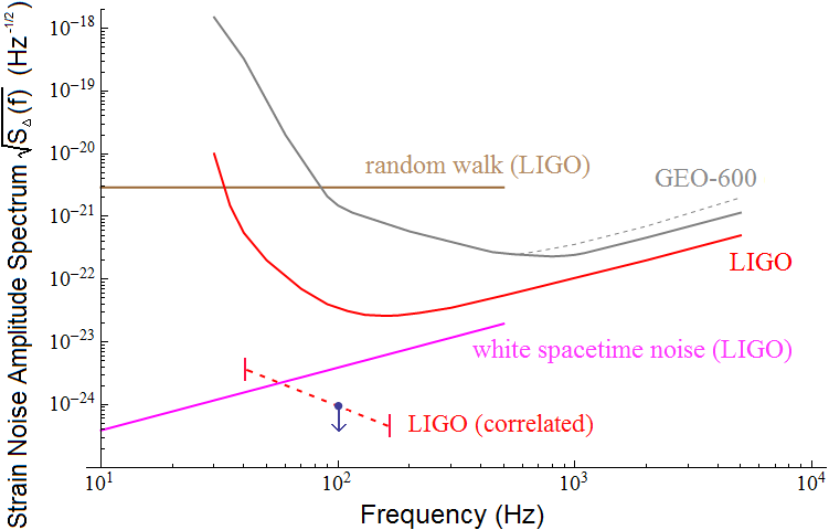
Figure 2: Spectra for strain amplitudes in interferometers, assuming metric fluctuations on classical determinate spacetime. The latest published noise spectra are compared against the predictions from models. Absolute normalizations for noise predictions are rough estimates only. The dashed line for GEO-600 is the sensitivity before light-squeezing techniques were applied. Since all predictions are metric-based, they should be compared against the “correlated” data point for LIGO’s stochastic gravitational-wave background limit, obtained by cross-correlating two interferometers far apart. The LIGO Scientific Collaboration (2011); The LIGO Scientific Collaboration and The Virgo Collaboration (2010)

Currently the experiments closest to the Planckian or sub-Planckian sensitivity levels required to test the predictions listed in the previous sections are gravitational interferometers such as LIGO. Noise levels published by the LIGO collaboration rule out select classes of metric-based noise predictions. The LIGO collaboration previously reported that it had achieved a strain noise of $3\times 10^{-23}\textrm{Hz}^{-1/2}$ around 100Hz in a single interferometerThe LIGO Scientific Collaboration and The Virgo Collaboration (2009). Also, by cross-correlating signals from pairs of interferometers separated by a large distance (the two 4-km LIGO detectors), the LIGO and Virgo collaborations obtained a more stringent bound on the stochastic gravitational-wave background, which may be used to set an upper limit on metric fluctuations as a source of noise. As long as the effects of Planckian fluctuations can be described in terms of a fluctuating metric, these limits can be carried over into limits on Planckian physics.

The cross-correlations here are of a different nature than the cross-correlations used in the Holometer, which are explained in a later section. In the case of a stochastic gravitational-wave background, as long as two detectors are within a distance smaller than the wavelength of the gravitational wave (on the order of $10^{6}\textrm{m}$ for a $100\textrm{Hz}$ wave), they show a coherent response to strains in the metric. LIGO and Virgo take the measured signals from two interferometers $s_{1}(t)$ and $s_{2}(t)$ and generate a time-integrated product signal $S\equiv\intop_{-T/2}^{T/2}dt\>s_{1}(t)s_{2}(t)$ Allen and Romano (1999). The two measured signals are each a mixture of metric strains and instrument noise, but $\left\langle S\right\rangle$ measures the correlated strain, while $\sqrt{\left\langle S^{2}\right\rangle-\left\langle S\right\rangle{}^{2}}$ measures the uncorrelated noise.

The gravitational wave energy density is defined as:

$$\Omega_{GW}(f)=\frac{f}{\rho_{c}}\frac{\mathrm{\mathrm{\textrm{d}}}\rho_{GW}}{\mathit{\mathrm{d}}f}$$ (28)

$\Omega_{GW}(f)$ is characterized by a power law dependence on $f$ in most models of interest. By assuming a frequency-independent spectrum over the frequency band $41.5-169.25\textrm{Hz}$, LIGO and Virgo obtained a result of $\Omega_{GW}<5.6\times 10^{-6}$ at 95% confidenceThe LIGO Scientific Collaboration and The Virgo Collaboration (2014). Using the relationshipThe LIGO Scientific Collaboration (2009),

$$\sqrt{S_{\Delta}(f)}=4\times 10^{-22}\sqrt{\Omega_{GW}}\left(\frac{100\textrm{Hz}}{f}\right)^{\frac{3}{2}}\textrm{Hz}^{-\frac{1}{2}}$$ (29)

this corresponds to a strain noise of $9.5\times 10^{-25}\textrm{Hz}^{-1/2}$.

Referring to Figure 2 and the $\sqrt{S_{\Delta}(f)}$ column of Table 1, it is clear that the “random walk” model is now safely ruled out. There were previous assertions that this model was ruled out by the Caltech 40-meter interferometer dataAmelino-Camelia (1999); *AmelinoCamelia2000; Ng and van Dam (2000), but as discussed in the previous section, such claims were results of incorrect straightforward comparisons between the predicted raw spacetime noise $\sqrt{S(f)}$ and the noise levels measurable specifically in interferometers, which should correspond to $\sqrt{S_{\Delta}(f)}$. Also notable is that the “white spacetime noise” model, approximating a class of possibilities in which the strain spectrum of the raw spatial noise is not dependent on the characteristics of the apparatus, is also probably ruled out: the 95% upper bound established by LIGO and Virgo is apparently lower than the predicted level of noise. However the quoted expression for $S(f)$ was only an estimate and equation (19) contains an uncalibrated scalar normalization factor that could be numerically much less than unity. We calculate the limit on this coefficient as $a_{0}<0.06$, with the same 95% confidence level. The sensitivity of the LIGO system continues to improve, and is expected to lead to better limits in the future The LIGO Scientific Collaboration and The Virgo Collaboration (2016a, b). The “one-third power” model is still out of reach, but could be within reach of proposed space interferometers such as eLISA. The simple “minimum uncertainty” model is quite far out of reach. Our prediction based on a zero-point field theory calculation also gives a result that is too small for any foreseeable experimental project. Again, all of the alternative metric fluctuation-based models are able to generate larger macroscopic effects only by suggesting non-standard coherence that is not present in standard field theory of Planckian metric fluctuations.

Other phenomenological approaches have considered different fundamental length scales for quantum gravity effects, for example by using the string length instead of the Planck lengthAmelino-Camelia (2001a); *AmelinoCamelia2001a. This would increase the predicted noise level slightly, although not to an extent that would significantly change our conclusions about exclusion of models.

II.5 Other Constraints Without Macroscopic Coherence

We have previously stated that these meta-models of metric based fluctuations make non-standard assumptions of coherence in order to generate macroscopically measurable effects. Without such assumptions, any noise that scales with distance would eventually result in locally measurable effects, making it difficult to preserve locality. There is now an experimental bound on such effects, established from the sharpness of optical images seen in telescopes and most stringently improved by observing TeV $\gamma$-rays using Cherenkov telescopesPerlman et al. (2015). If photons from a faraway source were subject to uncertainties that scale with the distance of travel, without an additional assumption of macroscopic coherence, the local images we take (at the telescope) of the source would suffer a loss of resolution. The clarity of these images can be used to place a general upper bound on any strain noise that scales as $\sigma\approx l_{P}^{\alpha}\mathcal{L}^{1-\alpha}$, at $\alpha\apprge 0.72$, which rules out both the “random walk” model and the “one-third power” model if we consider them without macroscopic coherence.

This constraint demonstrates the difficulty of satisfying the holographic information bound while considering spacetime degrees of freedom. Unlike in local field theories that attain holographic scaling of information through dualities (ignoring infrared paradoxesCohen et al. (1999)), quantum geometric states dominate the field ones in number once they are counted (e.g. statistical models of gravity Jacobson (1995); Verlinde (2011)). Examples like the “one-third power” model suggest that quantum geometric uncertainties must scale with system size in order to sufficiently limit the total degree of freedom. But an uncertainty that scales with distance makes it difficult to create a model that preserves locality, not to mention that a directionally isotropic strain noise such as the “one-third power” model violates the fundamental requirement of diffeomorphism covariance usually present in theories of spacetime.

III Holographic Fluctuations

III.1 Theory of Planckian Directional Entanglement

III.1.1 Theoretical Motivation

All effective theories treated thus far have assumed a classical determinate structure of spacetime and considered metric fluctuations within that structure. However, there are motivations to relax this assumption.

The theory of black holes suggests that the fundamental degrees of freedom present within a region of spacetime is not an extensive quantity but instead limited by the area of a surface bounding a given volume, measured in Planck unitsBardeen et al. (1973); Bekenstein (1972, 1973, 1974); Hawking (1974, 1975). Since it is well-known from considerations of quantum mechanical unitaritySusskind (1995); ’t Hooft (1993) that black holes are objects of maximal entropy, it makes sense to consider the two-dimensional entropy of black holes as an upper limit on the entropy contained within any given volume. Such arguments have led to a Lorentz covariant entropy bound that generalizes the same principles into a more precise upper limit, known as the Holographic Principle or Covariant Entropy Bound: the area of an arbitrary bounding surface in Planck units must be larger than the entropy contained throughout light sheets enclosed by that surfaceFischler and Susskind (1998); Bousso (1999a, b, 2002). This projection of internal degrees of freedom onto bounding surfaces inspires a nonlocal formulation of fundamental physics, as exemplified by the entanglement across spacelike separations in basic quantum mechanics, that imposes a Planckian bound on quantum degrees of freedom stored within spacetime (which dominate the entropic budget).

Hogan has previously suggested a phenomenological model of how such holographic bounds might be manifested in the real universeHogan (2012a, 2008a, 2008b, 2009, b, c); Hogan and Jackson (2009); Hogan (2013), leading to an exotic kind of position fluctuation called “holographic noise.” In this model, the nonlocality discussed above arises in a spacetime that is not a fundamental entity but rather an emergent phenomenon in systems much larger than the Planck scale. A classical concept of spacetime involves pointlike events on a determinate manifold, continuously mapped onto real coordinates. But in quantum mechanics, “position” is a property represented by an operator acting on a Hilbert space. An added assumption of a definite background usually leads to contradictions with gravityCohen et al. (1999); Rovelli (2004); Ashtekar (2011), and there are arguments that the metric should also be considered an emergent entityBanks (2011); Banks and Kehayias (2011). Here, a Hilbert space describes the background spacetime degrees of freedom, and operators that act on such a Hilbert space generate positions of massive bodies.

In a wave picture, spatial information is carried by null waves, and the Hilbert space describing spacetime degrees of freedom “collapses” when null surfaces interact with matter. The waves are Planck bandwidth-limited, so they are fundamentally indeterminate in directional resolution and transverse localizationHogan (2013).

A simple, well controlled model of such a geometrical state can also be expressed by a commutator of geometrical operators $\hat{x}_{\mu}$ that approximate classical 4-position coordinates of a body, including time, in the macroscopic limitHogan (2012b, c, a). We write a manifestly Lorentz-covariant 4-dimensional formulation of the commutatorHogan (2012c):

$$\left[\hat{x}_{\mu},\hat{x}_{\nu}\right]= i\frac{1}{2\sqrt{\pi}}\hat{x}^{\kappa}\hat{U}^{\lambda}\epsilon_{\mu\nu\kappa\lambda}l_{p}$$ (30)

$$\textrm{where}\quad\hat{U}^{\lambda}\equiv\frac{\dot{\hat{x}}^{\lambda}}{\sqrt{\dot{\hat{x}}_{\alpha}\dot{\hat{x}}^{\alpha}}},\quad\dot{\hat{x}}\equiv\frac{\partial\hat{x}}{\partial\tau}$$ (31)

Here $\hat{U}^{\lambda}$ represents an operator in the same form as the dimensionless 4-velocity of a body, and $\tau$ denotes proper time.

The $\hat{x}_{\mu}$ are not coordinate variables, but rather operators acting on a Hilbert space from which spacetime emerges. This is not conventional quantum mechanics, in which operators describe the position of microscopic bodies within a classical spacetime. Instead, these operators describe the spacetime positions of macroscopic objects, ignoring in this approximation standard quantum mechanics as well as gravity. Thus it is not a fundamental theory, but gives an effective model of quantum geometry, that agrees with gravitational bounds on directional information. In this model, spacetime itself can undergo quantum entanglement.

Strangely, $\hat{x}_{0}$ is an operator that represents proper time, but is not exactly the classical time variable. This proper time operator does not commute with the space operators, and therefore implies slightly different clocks in different spatial directions. Since an interferometer can be thought of as light clocks in two orthogonal directions, this commutator model lends itself well to measurement with an interferometer. We have seen that the two orthogonal macroscopic arms of a Michelson interferometer contain coherent states of photons that are spatially extendedThe LIGO Scientific Collaboration (2011).

While this commutator describes a quantum relationship between macroscopically separated world lines based on relative position and velocity, we still require that causality remains consistent. Causal diamonds surround every timelike trajectory, and an approximately classical spacetime emerges that is consistent wherever the causal diamonds overlap.

III.1.2 Normalization of Holographic Position Fluctuations

To estimate a precise normalization of this model, take a rest frame limit

$$\left[\hat{x}_{i},\hat{x}_{j}\right]=i\frac{1}{2\sqrt{\pi}}l_{p}\epsilon_{ijk}\hat{x}_{k}$$ (32)

Equation (32) is a spin algebra-like representation of holographic information that can be used to count precisely the degrees of freedom present in a 2-sphereHogan (2012c). Consider $\left|l\right\rangle$, a radial spatial separation eigenstate of two bodies separated by a distance $L$, labeled by its quantum number.

$$\left|\hat{x}\right|^{2}\left|l\right\rangle=\frac{1}{4\pi}l(l+1)l{}_{p}^{2}\left|l\right\rangle=L^{2}\left|l\right\rangle$$ (33)

Within a 2-sphere of radius $R=\frac{1}{2\sqrt{\pi}}\sqrt{l_{R}(l_{R}+1)}l_{p}$ exist $l_{R}$ discrete radial position eigenstates ($1\leq l\leq l_{R}$). Each of them have $2l+1$ eigenstates of direction:

$$N_{2S}=\underset{l=1}{\overset{l_{R}}{\sum}}(2l+1)=l_{R}(l_{R}+2)\approx 4\pi\left(\frac{R}{l_{p}}\right)^{2}$$ (34)

The numerical coefficient is chosen to agree with emergent spacetime theories that describe gravity entropicallyVerlinde (2011). For a length measurement of scale $\mathcal{L}$, this gives a precisely characterized transverse mean square position uncertainty of

$$\langle\Delta x_{\perp}^{2}\rangle={\frac{1}{2\sqrt{\pi}}l_{p}\mathcal{L}},$$ (35)

which increases with scale.

III.1.3 Properties of Holographic Position Noise

The sections that follow estimate the signal response in various interferometer architectures. Because a metric with classical position coordinates is not assumed, a holistic analysis is required of the system that includes the apparatus and the emergent geometry it resides in: a quantum-geometrical system of matter and light. Instead of a fluctuating metric as in the previous sections, we adopt the following phenomenological model of matter position and light propagation in an emergent space-time:

1. Light propagates in the vacuum of emergent spacetime as if it is classical and conformally flat. Thus, longitudinal propagation and photon quantum shot noise are standard.

2. In the nonrelativistic limit, the position of matter is described by a wavefunction that represents spatial information in the geometry, with a transverse width estimated in in (35). This is not standard quantum mechanics: it is a geometrical wavefunction shared by bodies close together in space, separated by much less than $\mathcal{L}$.

3. Position becomes definite relative to an observer— any timelike world-line— when the Hilbert space of the quantum geometry “collapses”, as null wave fronts, propagating in causal diamonds around the observer, interact with other matter on null surfaces. The finite wave function width thus gives rise to coherent fluctuations in transverse position, as well as emergent locality: nearby bodies fluctuate together with each other, relative to distant ones. (Here, “null” is used to describe a set of events that have lightlike separation from an observer’s worldline.)

III.1.4 Relationship Between Planckian Directional Entanglement and Other Violations of Relativity

In this model of quantum geometry, localized spatial position coordinates do not have an exact physical meaning, but emerge from the quantum system. While the commutation relation is covariant and has no preferred direction, timelike surfaces are now frame-dependent in ways that describe the observer-dependence of a spacetime. The system violates Lorentz invariance, but as mentioned in the introduction, is within established experimental bounds. It leads to a directional uncertainty that decreases with separation. Thus the model reduces to classical geometry in the macroscopic limit.

Thus, the conjectured model is Lorentz covariant, but it is not Lorentz invariant. The violation of Lorentz invariance here is qualitatively different from previously investigated possible effects, such as those predicted by some effective field theoriesMattingly (2005). This type of Lorentz violation does not result in any dispersive change in photon propagation. Null particles of any energy in any one direction propagate exactly according to normal special relativity, consistent with current experimental limits from cosmic observations of gamma ray bursts with the Fermi/GLAST satelliteAbdo et al. (2009). The energy non-dependence of polarization position angle agrees with INTEGRAL/IBIS satellite boundsLaurent et al. (2011), and we do not propose any kind of dispersive effect on the propagation of massive particles that could be tested by cold-atom interferometersAmelino-Camelia et al. (2009).

Several recent proposals have suggested experimentally testable mascroscopic phenomena involving gravity within the framework of traditional quantum mechanics. One idea is to calculate and observe the quantum evolution of the center of mass of a many-body system within a classical spacetimeYang et al. (2013), which is clearly distinct from the type of quantum spacetime we are proposing. Another is to create and study quantum superposition states of many-particle systems extended across macroscopic spatial distancesMarshall et al. (2003); Romero-Isart et al. (2011), which is different from the entanglement of spatial degrees of freedom we are discussing. Lastly, there is a proposal to probe the canonical commutation relation of the center-of-mass mode of a massive object using quantum optics, assuming certain modifications to the Heisenberg uncertainty relation arising from Planck-scale spacetime uncertaintiesPikovski et al. (2012). This type of experiment is suited to test the kind of meta-models surveyed in section II.2, especially the “minimum uncertainty” one, but not the type of transverse effect we are hypothesizing.

The phenomena discussed here are of course distinct from potential effects of primordial gravitational-wave backgroundsMaggiore (2000). The new physics proposed also differs from microscopic non-commutative directional uncertainties in models that consider gravity as the gauge theory of the deSitter group, in which Planck’s constant is kinematically introduced into gravity through non-commutative generatorsTownsend (1977); Maggiore (1993). These ideas have not led to an effective theory that describes a macroscopically manifested phenomenon.

III.2 Predictions for Noise in Interferometers

III.2.1 Holometer: Simple Michelson

As previously mentioned, Fermilab is commissioning an experimental apparatus designed to be particularly sensitive to this type of spacetime uncertainty, named the Holometer. This experiment uses a simple Michelson interferometer configuration, but is sensitive to rapid Planckian transverse position fluctuations on a light-crossing time, whose spatial coherence is shaped by causal structure, as expected for holographic noise.

To predict the noise profile measured in a Michelson interferometer, we again need to consider the reflections off of the beam splitter at two different times. Because we are positing a noncommutative spacetime with an uncertainty of transverse nature, the one-dimensional formulation in (26) is now insufficient. An idealized Michelson interferometer in a classical geometry, with arms oriented in the 1 and 2 directions, actually measures the following macroscopic quantity:

$$X(t)=\hat{x}_{2}(t)-\hat{x}_{1}(t-2L/c)$$ (36)

We will approximate the continuous interaction of matter with null waves as a series of discrete measurements separated by Planck times, over which a transverse Planckian random walk accumulatesHogan (2012a). We will give two predictions, a baseline prediction based on the most likely interpretation of the theory and a minimal prediction that assumes the most conservative limit on the accumulation of spacetime uncertainty between successive collapses of the wavefunction.

Baseline Prediction

We write down the autocorrelation function for the arm-length difference X(t) at time lag $\tau$ in the following form:

$$\Xi(\tau) =\left\langle X(t)X(t+\tau)\right\rangle$$ (37)

$$=\begin{cases}\frac{ct_{p}}{2\sqrt{\pi}}(2L-c\left|\tau\right|)&0<c\left|\tau\right|<2L\\ 0&c\left|\tau\right|>2L\end{cases}$$ (38)

Detailed explanations of these calculations are laid out in previous papers and need not be repeated here, but the justification for (38) is fairly straightforward. The aforementioned considerations of an emergent spacetime obeying causal structures leads us to conclude that this holographic random walk is bounded by the light round trip time 2L/c, as causal boundaries dictate this to be the longest time interval during which the relative phases in transverse directions deviate before the “memory” is “reset” (see Figure 3). In concluding this, we are assuming that the spacetime degrees of freedom in the transverse direction do not collapse upon the interaction of the information-carrying null waves with the end mirrors, and that these null waves complete the two-way trips between the beam splitter and the end mirrors while retaining this information. Once we establish that the autocorrelation $\Xi(\tau)$ must decrease to zero at 2L/c, it is straightforward to conclude that the function must decrease linearly from its peak value at zero lag in order to contain causal diamonds and reflect causal structure in a scale-invariant way.

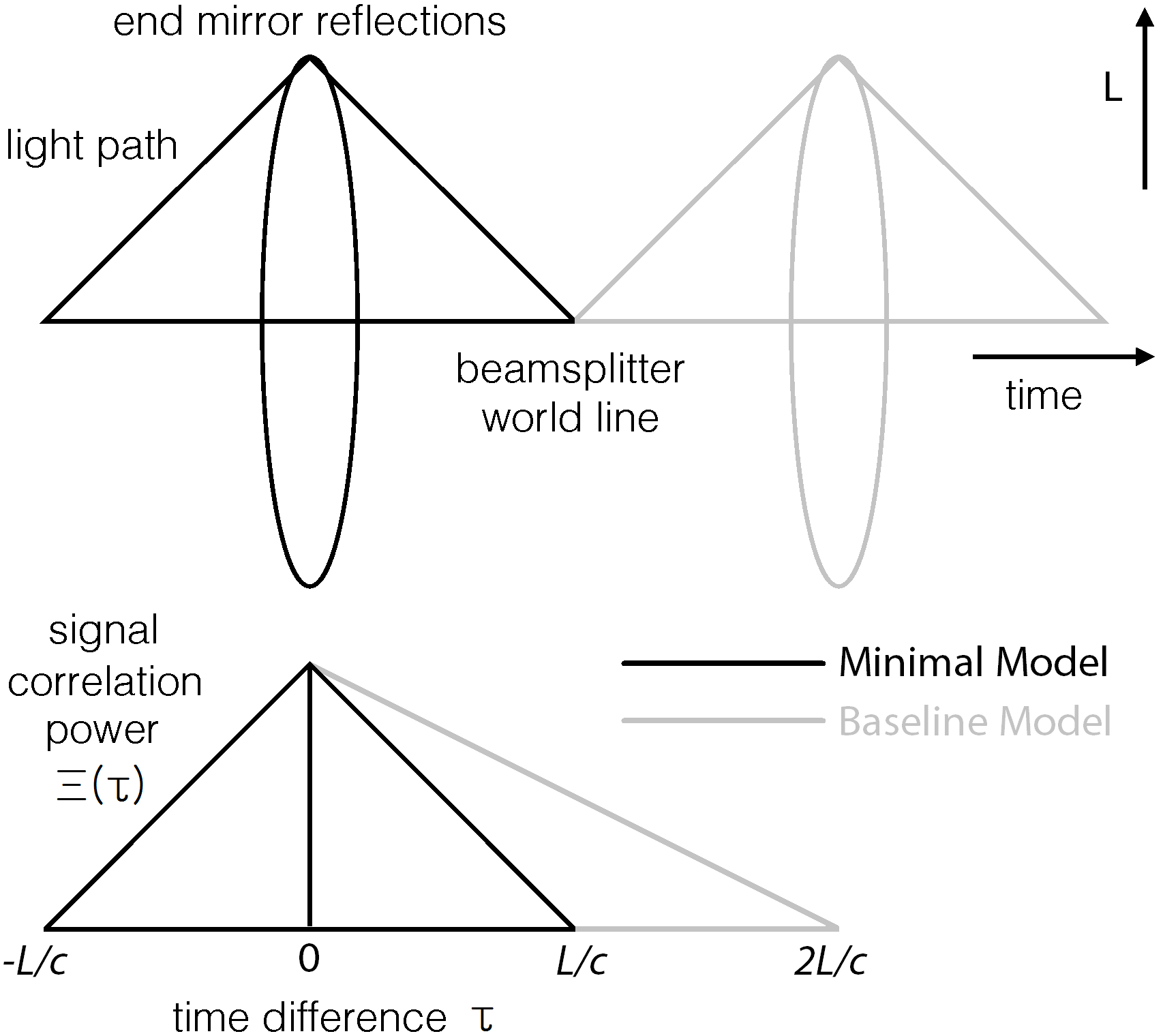
Figure 3: Causal structures of the baseline and minimal models compared, along with the corresponding behavior in the signal power of the autocorrelation in differential arm length. Barely overlapping causal diamonds of two interferometers separated in time by $2L/c$ leads to a correlation in the baseline model, but in the minimal model, the causal diamond of a single interferometer acts as the causal boundary for the correlation signal, a minimal departure from classicality.

Figure 4: Predicted noise spectra for the Holometer from Planckian directional entanglement using two different models, calculated in eq. (40) and eq. (43). For 40m arms, the low-frequency limits are $9.86\times 10^{-21}\textrm{m/$\sqrt{\textrm{Hz}}$}$ and $6.98\times 10^{-21}\textrm{m/$\sqrt{\textrm{Hz}}$}$. The minimal model has a low-frequency value that is smaller by $1/\sqrt{2}$, but the first zero occurs at a frequency twice as large compared to the baseline model.

The zero-lag value in (38) naturally follows from (32) and (35), but it is important to clarify that the value does not represent the propagation of one null wave over a distance 2L despite its algebraic appearance. Since X(t) represents the arm-length difference, each arm contributes its own uncorrelated portion of the total variance. The uncertainty posited is fundamental to the spacetime itself—that is, the positions of massive bodies, such as mirrors—and not applied to the spatial propagation of light, which is not susceptible to the transverse fluctuations. The information-carrying null waves only accummulate transverse uncertainties over the physical distance of a single arm length L even though the light beam travels a distance of 2L. The two reflections off of the beam splitter respectively measure its location in two orthogonal directions at two different times, and with each transverse reflection manifests a spatial uncertainty in the direction transverse to the one being measured.

The corresponding spectrum in the frequency domain is calculated by the cosine transform (see Figure 4) Hogan (2012a):

$$\tilde{\Xi}(f) =2\int_{0}^{\infty}\textrm{d}\tau\Xi(\tau)\cos(2\pi f\tau)$$ (39)

$$=\frac{c^{2}t_{p}}{\sqrt{\pi}(2\pi f)^{2}}\left[1-\cos(f/f_{c})\right],\quad f_{c}\equiv\frac{c}{4\pi L}$$ (40)

$$\tilde{\Xi}(f\ll f_{c}) =\frac{2}{\sqrt{\pi}}t_{p}L^{2}$$

$$=[2.47\times 10^{-22}\textrm{Hz}^{-\frac{1}{2}}]^{2}\cdot L^{2}$$ (41)

As discussed below in more detail, the actual Holometer experiment design includes another feature that is not described by this simple Michelson model: its signal is obtained by cross-correlating the outputs of dual interferometers in a nested configuration. Due to entanglement, if the separation is much smaller than the size of the apparatus, the cross signal approximates the autospectrum estimated here: the beam splitters of the two interferometers “move together” because the light paths encompass the same region of space-time and their emergent geometries collapse into the same position state.

Recall the fact that a random walk metric fluctuation resulted in a white noise spectrum in section II.3. Equation (40) also gives the same flat spectrum (up to a shoulder around inverse light travel time). However, the different physical assumptions about the origin of the noise lead to different predictions for other interferometer architectures. The coherent quantum and transverse nature of holographic fluctuations lead to counterintuitive behavior that cannot be reproduced in a model based on a fluctuating metric.

Minimal Prediction

In generating the baseline prediction, we made one assumption that is not obvious from the principles laid out in section III.1.3. We now consider the alternative possibility that the spacetime degrees of freedom collapses in the transverse directions upon the interaction of the information-carrying null waves with the end mirrors. The end mirrors have the effect of isolating the quantum uncertainty of the spacetime inside the apparatus from its uncertainty relative to the outside (see Figure 3). Earlier we considered these null waves making two-way trips between the beam splitter and the end mirrors, but in actuality, we are talking about a conception of emergent spacetime that is covered by these null waves carrying wavefunctions of transverse quantum uncertainty, at all points in spacetime and in all directions. Simply consider only the incoming waves from the end mirrors to the beam splitter, and the time-domain autocorrelation for X(t) changes to:

$$\Xi(\tau) =\begin{cases}\frac{ct_{p}}{\sqrt{\pi}}(L-c\left|\tau\right|)&0<c\left|\tau\right|<L\\ 0&c\left|\tau\right|>L\end{cases}$$ (42)

The only difference here is that the “memory” has been reduced to a single arm length. The zero-lag value and the linear triangular shape of the function remains unchanged. The corresponding spectrum in the frequency domain is given by (see Figure 4):

$$\tilde{\Xi}(f) =\frac{2c^{2}t_{p}}{\sqrt{\pi}(2\pi f)^{2}}\left[1-\cos(f/f_{c}^{0})\right],\quad f_{c}^{0}\equiv\frac{c}{2\pi L}$$ (43)

$$\tilde{\Xi}(f\ll f_{c}^{0}) =\frac{1}{\sqrt{\pi}}t_{p}L^{2}$$

$$=[1.74\times 10^{-22}\textrm{Hz}^{-\frac{1}{2}}]^{2}\cdot L^{2}$$ (44)

III.2.2 GEO-600: Interferometer with Folded Arms

As there are several interferometric experiments at or close to Planck sensitivity, it is important to generate consistent predictions for those experiments in order to make sure that this hypothesis is not already ruled out. Here we will focus on two of the most sensitive experiments, first GEO-600 and then LIGO in the following section. We will be mostly following the assumptions made for the baseline prediction in the previous section.

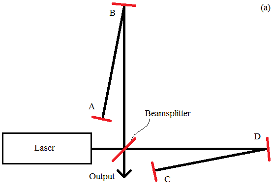
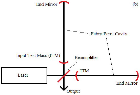
Figure 5: (a) Schematic diagram of GEO-600. (b) Schematic diagram of LIGO.

The GEO-600 detector uses a Michelson interferometer with each arm folded once to double the distance traveled by the light (see Figure 5(a)). In such a case, we expect the “memory” to last twice as long. But the actual physical distance being measured is still just a single L, and the holographic noise only accumulates over a single arm length, starting or ending at the beam splitter. Again, the uncertainty is fundamental to the spacetime itself and not subject on the light propagating through space. A transverse uncertainty is manifest in each measurement of the relative distance between two objects, the beam splitter (BS) and either one of the two end mirrors (B and D). This directional entanglement only results in observable noise at instances of orthogonal reflection of the light, which happens twice at the beam splitter.

One might raise the objection that if these hypothesized uncertainties are inherent to the fabric of spacetime itself, the mirrors near the beam splitter (A and C) should appear to move coherently with the beam splitter, allowing the device to accumulate spatial noise over the full length of the folded arm. In fact, such posited spacetime coherency is integral to the design of the Holometer. But for the GEO-600 setup, this coherence would not affect the contribution of folded arms to the signal.

As mentioned in the previous section, we may see the interferometer as a pair of independent orthogonal light clocks and consider the delocalized quantum modes extended within the arms. Consider the fact that the proper time operator does not commute with either of the two non-commuting orthogonal space operators, and it becomes clear that a transverse uncertainty is manifest only upon the measurement of a single non-folded arm length. For example, when the distance between the BS and B is being measured, the horizontal arm comprised of C, D, and the BS acts as a light clock. Its horizontal position (and the associated uncertainty), transverse to the vertical distance being measured, is coherent within causal bounds.

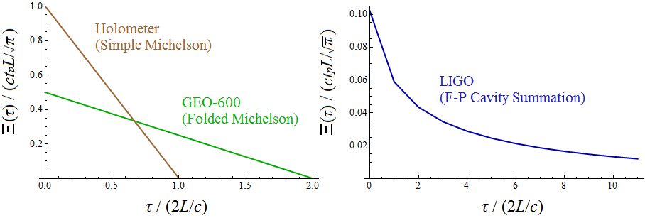
Figure 6: Plots of time-domain autocorrelation functions for X(t) at time lag $\tau$, using the baseline model: eq. (38) for the Holometer, eq. (46) for GEO-600, and eq. (50) for LIGO. All axes have been normalized to the same appropriate unitless scale to provide a clear comparison between different interferometer configurations independent of experimental parameters. The simple Michelson configuration has a $\Xi(\tau=0)$ value that shows the random walk variance in (35) applied over two independent arm lengths, along with a time memory of one light round trip time over one arm length. The folded Michelson configuration has a time memory that lasts over two light round trip times but preserves the same area underneath the function. The model for an interferometer with Fabry-Perot cavities uses a probabilistic summation of the autocorrelation functions for Michelson interferometers with arms that are folded multiple times.

For a semi-classical explanation, consider localized modes of the information-carrying null waves. In this formulation, the quantum wavefunction of the geometry collapses every time the null waves interact with matter (e.g. a mirror) even though the actual measurement is made only when the photon is observed. Consider looking at the interferometer from the perspective of B and observing the location of the BS (and A) via a null wave along the vertical arm. This reference null wave accumulates transverse phase uncertainty over a single vertical arm length. From this perspective we can consider the horizontal arm as a light clock, and indeed the transverse (horizontal) uncertainty at the BS is coherently applicable to C, as the distance between the two is well within the causal bounds established by the travel time of said vertical null wave.

However, consider a light beam that has just reflected off of C and traveling towards D. As the light beam makes the trip over the length of the horizontal arm, we can imagine another null wave that carries the information about the horizontal deviation at C (transverse to the reference null wave) also making the same trip and reaching D at the same time as the light beam. Thus, the uncertainties in the horizontal positions of the BS or C do not affect the travel time of the horizontal light beam during 3/4 of the beam’s propagation within the arm. The transverse (horizontal) uncertainty really only comes into play on 1/4 of the beam path, as the reference null wave measures the vertical distance from B to the BS and the relative transverse uncertainty created affects the light beam’s travel time between D and the BS.

We can now conclude that the low-frequency limit of the displacement amplitude spectrum $\tilde{\Xi}(f)$ calculated in eq. (41) must remain the same despite the folded arms, because at frequencies much below inverse light storage time the phenomenon described must behave almost “classically,” and the extended “memory” should not affect the measured uncertainty at all. If we imagine a simple Michelson interferometer co-occupying the space of the GEO-600 detector in parallel configuration, the two devices should demonstrate equal phase noise at such low frequencies. These requirements lead us to write (see Figure 6):

$$X(t)= \hat{x}_{2}(t)-\hat{x}_{1}(t-4L/c)$$ (45)

$$\Xi(\tau)= \left\langle X(t)X(t+\tau)\right\rangle$$

$$= \begin{cases}\frac{1}{2^{2}}\frac{ct_{p}}{2\sqrt{\pi}}(2\cdot 2L-c\left|\tau\right|)&0<c\left|\tau\right|<4L\\ 0&c\left|\tau\right|>4L\end{cases}$$ (46)

$$\tilde{\Xi}(f)= \frac{1}{2^{2}}\frac{c^{2}t_{p}}{\sqrt{\pi}(2\pi f)^{2}}\left[1-\cos(f/f^{\prime}_{c})\right]$$ (47)

$$\textrm{where }f^{\prime}_{c}\equiv\frac{1}{2}\frac{c}{4\pi L}$$

This gives the same low-frequency limit as equation (41).

We still cannot simply compare this prediction to the noise in differential arm length measured at GEO-600, because noise from metric fluctuations behaves differently from this posited holographic noise. Experiments designed for gravitational waves look for strains in the metric applied to the entire arm length and the entire light path. They assume that the perturbation in the location of the beam splitter is coherent with those of the inboard mirrors (e.g. A and C in Figure 5(a)) in all spatial directions, and hence can claim an increase in sensitivity by reflecting light back and forth within the arms. GEO-600 attains a twofold enhancement in sensitivity at low frequencies (relative to inverse light storage time) by making the laser beam do two round trips within each arm, during which the strain in the metric will affect a light path that is twice as long. But for the kind of directional entanglement based on the assumptions in section III.1.3, the inboard mirrors no longer contribute the same noise as the beam splitters, for reasons laid out in detail above. This means that for the purposes of measuring the effects of this noncommutative emergent spacetime, for frequencies lower than inverse light storage time $f=c/4L$ (to account for the extended “memory”) we must correct the sensitivity of GEO-600 data by a factor of $\frac{1}{2}$ (i.e. multiply the position noise level by a factor of 2). Since the light storage time in the arms is quite short, this correction applies to the spectrum of GEO-600 over the entire relevant frequency range. (For this design, we do not count the “storage time” represented by the entire power-recycled cavity, only that between encounters with the beamsplitter.)

If we convert the holographic noise prediction into a gravitational wave strain equivalent expected to be observed in GEO-600 (instead of correcting the sensitivity of GEO-600 data for holographic noise), we get:

$$\tilde{h}_{eq}(f\ll f^{\prime}_{c}) =\frac{1}{2}\cdot\frac{\sqrt{\tilde{\Xi}(f\ll f^{\prime}_{c})}}{L}=\frac{1}{2}\sqrt{\frac{2t_{p}}{\sqrt{\pi}}}$$ (48)

$$=1.23\times 10^{-22}\textrm{Hz}^{-\frac{1}{2}}$$

In the case of the minimal model, the folded arms of GEO-600 does nothing to change the causal structure of the system (including the length of the “memory”) or the low-frequency amplitude of the displacement spectrum. So the time and frequency-domain behaviors take the exact same functional forms as the minimal prediction for the simple Michelson configuration of the Holometer, equations (42)$\sim$(44), simply numerically adjusted for the longer 600m arm length. Converted to a gravitational wave strain equivalent, we get $\tilde{h}_{eq}(f\ll f_{c}^{0})=\frac{1}{2}\sqrt{t_{p}/\sqrt{\pi}}=8.72\times 10^{-23}\textrm{Hz}^{-\frac{1}{2}}$.

III.2.3 LIGO: Interferometer with Fabry-Perot Cavities

The prediction for LIGO is subject to more complications than the GEO-600 example. The detector uses Fabry-Perot (F-P) cavities within each arm with average light storage times (for the device as used in published bounds) of $r=35.6$ light round tripsThe LIGO Scientific Collaboration (2009) (see Figure 5(b)). We need to devise a simple model of the response such a system has to holographic noise.

We will work within the assumptions of the baseline model. Think of each incoming light wavefront as having an exponentially decreasing probability $\textrm{e}^{-(n-1)/r}$ of making at least n round trips within the cavity, and sum the contribution of each possibility to the total noise. A natural extension of the arguments made for the 2 round trips within a GEO-600 arm gives (see Figure 6):

$$\Xi(\tau)= \sum_{n=1}^{\infty}(\textrm{e}^{-(n-1)/r}-\textrm{e}^{-n/r})$$

$$\times\begin{cases}\frac{1}{n^{2}}\frac{ct_{p}}{2\sqrt{\pi}}(2nL-c\left|\tau\right|)&0<c\left|\tau\right|<2nL\\ 0&c\left|\tau\right|>2nL\end{cases}$$ (49)

$$\tilde{\Xi}(f)= \sum_{n=1}^{\infty}(\textrm{e}^{-(n-1)/r}-\textrm{e}^{-n/r})$$

$$\times\frac{1}{n^{2}}\frac{c^{2}t_{p}}{\sqrt{\pi}(2\pi f)^{2}}\left[1-\cos(f/f{}_{c}^{(n)})\right]$$ (50)

$$\textrm{where }f_{c}^{(n)}\equiv\frac{1}{n}\frac{c}{4\pi L}$$

The low-frequency limit is still equal to equation (41).

However, in constructing the model above, we introduced an additional assumption that these nonlocal modes of light respond coherently to holographic noise. While it is tempting to think of localized light being “reflected” or “transmitted” by the input test mass (ITM), the actual quantum modes in the system are of course delocalized. A model of localized light modes can accurately be used to describe a light cavity responding to time-fluctuations in the metric, as long as we build into our calculations the time delays after each successive reflection. But this implcitly assumes that there is only one “clock,” and for this type of noise generated by a quantum spacetime, there are two independent clocks in noncommuting orthogonal directions. Therefore the fact that the quantum wavefunction of the geometry collapses after each interaction of null waves with matter invalidates such a classical calculation. So without a rigorously formulated structure for this emergent spacetime, let alone a precise quantum mechanical description of how these null wave modes interact with matter, it is unclear that this model gives an accurate description of the actual physical phenomenon.

We could instead think of delocalized light modes being stored within the cavity for an extended period of time before collapsing outside of the cavity, hence averaging the position variance present at the beam splitter across a longer period of time. Such considerations lead us to suggest eq. (50) only as a best guess, not a rigorous prediction of directional entanglement.

We also need to remove LIGO’s enhancement factor for gravitational waves that do not apply to the conjectured effects of directional entanglement. The correction here necessary to generate the applicable noise spectrum is much more involved than the GEO-600 case. LIGO’s light storage time is long enough that the correction factor is no longer constant across its entire measurement spectrum. Also, we might naively assume that an r-fold increase in light storage time would result in an r-fold enhancement in sensitivity to gravitational waves, but this is not actually the case. The sensitivity to gravitational wave strain is enhanced by a factor somewhat greater than r due to optical resonance. The transfer function from an optimally oriented and polarized gravitational wave strain to the optical phase shift measured at the laser output is given by (at low frequencies $f<c/4\pi L$) Meers (1988); Saulson (1994):

$$\frac{\phi}{h}(f)=\left(\frac{16\pi Lr}{\lambda}\right)\frac{1}{\sqrt{1+(8\pi fLr/c)^{2}}}$$ (51)

We have argued that at low frequencies, the predicted directional entanglement will manifest in a folded interferometer such as GEO-600 in a manner that seems almost “classical.” Since we used for LIGO a rough model of probabilistically summing up light packets that go through n round trips before exiting the Fabry-Perot cavities, we argue that at low frequencies LIGO also responds to holographic noise as if it was a simple Michelson interferometer. The transfer function for a simple Michelson interferometer operating at the low-frequency limit, given the same kind of optimally configured gravitational wave strain as above, is given by:

$$\frac{\phi_{0}}{h}(f\rightarrow 0)=\left(\frac{2\pi}{\lambda}\right)(2L)\cdot 2\cdot\frac{1}{2}$$ (52)

where the factor of 2 comes from the two arms contributing equal parts, and the $\frac{1}{2}$ comes from translating metric strain into length strain. This means that the sensitivity of LIGO is reduced by the following factor when measuring the uncertainty in beam splitter position due to holographic noise (instead of gravitational waves):

$$\frac{\phi}{\phi_{0}}(f)=\frac{4r}{\sqrt{1+(8\pi fLr/c)^{2}}}$$ (53)

The gravitational wave equivalent we expect to detect in LIGO can be calculated by writing

$$\tilde{h}_{eq}(f)=\frac{\sqrt{\tilde{\Xi}(f)}}{2\cdot\frac{1}{2}\cdot L}\left(\frac{\phi}{\phi_{0}}(f)\right)^{-1}$$ (54)

and substituting equations (50) and (53) into the expression.

Assuming the minimal model has rather drastic consequences for the LIGO case. The ITM creates a boundary condition that is defined very close to the beam splitter, where the quantum wavefunction containing the spacetime degrees of freedom would collapse. One could argue that the beam splitter never “sees” the entire arm and the end mirror, leading to a tiny undetectable holographic noise since the ITM is very close to the beam splitter. We discounted this possibility in the baseline model, citing the view that the arms can be regarded as (non-commuting) directional light clocks whose phases are compared at the beam splitter, but it cannot be conclusively ruled out.

III.3 Comparison with Experimental Data

III.3.1 Expected Sensitivity for the Holometer

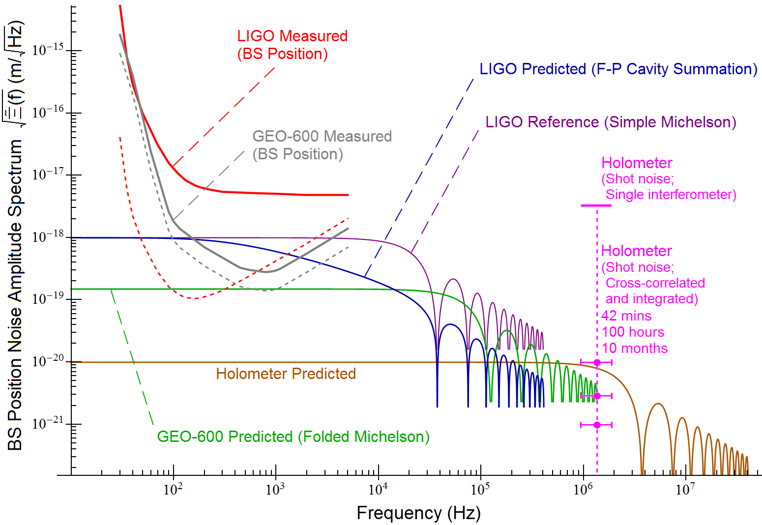
Figure 7: Spectra for beam splitter position fluctuations, assuming the noise source to be Planckian directional entanglement (baseline model). To give the appropriate reduced sensitivity in measuring such noise, we increase LIGO’s published noise levels for differential arm length by the sensitivity enhancement factor for gravitational wave strain calculated in (53). For GEO-600 data, the amplification factor is simply 2. The dashed lines represent uncorrected raw published noise curves. Predicted noise spectra are from eq. (47) for GEO-600 (folded Michelson), eq. (50) for LIGO (Fabry-Perot cavity), and eq. (40) for the Holometer (simple Michelson). Expected levels of flat shot noise are plotted for comparison, as the Holometer operates at a high enough frequency that we expect this noise source to dominate. By using an integration time that is N times longer than sampling time, with data from two overlapping interferometers, we can significantly reduce the uncorrelated shot noise by a factor of $1/\sqrt{N}$ while keeping the signal from correlated holographic noise constant. A frequency bin ranging from $f=c/8L$ to $c/4L$ is shown as an example. The LIGO Scientific Collaboration (2011); The LIGO Scientific Collaboration and The Virgo Collaboration (2010)

The Fermilab Holometer implements a design that is optimized to look for this noise from Planckian directional entanglement. By operating at high frequencies above 50kHz, it minimizes noise sources that are difficult to control such as seismic noise, thermal noise, or acoustic noiseWeiss (1972); Adhikari (2014); The LIGO Scientific Collaboration (2009). A flat Poisson shot noise dominates the spectrum at a phase spectral density ofA. Chou, R. Weiss et al. (2009) (Fermilab Holometer Collaboration); B. Kamai et al. (2013) (Fermilab Holometer Collaboration); A. Chou et al. (2015) (Fermilab Holometer Collaboration):

$$\Phi_{shot}=\frac{1}{\sqrt{\dot{n}_{BS}}}=\sqrt{\frac{E_{\gamma}}{P_{BS}}}=9.6\times 10^{-12}{\textstyle\textrm{rad}/\sqrt{\textrm{Hz}}}$$ (55)

where $\dot{n}_{BS}$ is the number of photons incident on the beam splitter per unit time, $E_{\gamma}=1.2\textrm{eV}$ is the energy of the infrared photons used, and $P_{BS}=2\textrm{kW}$ is the intracavity power of the laser after recycling. This noise is about a factor of 330 above the predicted signal from holographic fluctuations, calculated in (41) using the baseline model.

However, the Holometer is a set of two overlapping Michelson interferometers co-occupying almost the same space. If the holographic noise is inherent to the spacetime itself, we can reasonably expect the signal to be correlated across the two devices since the two beam splitters are close together, well within the causal bounds established by null wave travel times. In contrast, shot noise will obviously be uncorrelated. So we may write the phase fluctuations observed in the two detectors as $d\phi_{i}^{tot1}=d\phi_{i}^{corr}+d\phi_{i}^{uncorr1}$ and $d\phi_{i}^{tot2}=d\phi_{i}^{corr}+d\phi_{i}^{uncorr2}$, where $i$ indexes the data taken each sampling time. Therefore if we cross-correlate the measured fluctuations from the two interferometers and integrate over an extended period of time, the signal from the correlated noise from emergent quantum geometries will remain at a constant level, while the cross-correlation of the two uncorrelated shot noises will decrease by a factor of $1/\sqrt{N}$, where N is the ratio of the integration time over the sampling timeA. Chou, R. Weiss et al. (2009) (Fermilab Holometer Collaboration); B. Kamai et al. (2013) (Fermilab Holometer Collaboration); A. Chou et al. (2015) (Fermilab Holometer Collaboration):

$$d\phi_{i}^{tot1}\times d\phi_{i}^{tot2}$$

$$\quad\approx\frac{1}{N}\sum_{i}^{N}(d\phi_{i}^{corr}d\phi_{i}^{corr}+d\phi_{i}^{uncorr1}d\phi_{i}^{uncorr2})$$ (56)

$$\quad=\left\langle(d\phi^{corr})^{2}\right\rangle+\frac{2}{\pi}\frac{1}{\sqrt{N}}\left\langle(d\phi^{uncorr})^{2}\right\rangle$$ (57)

where $2/\pi$ is the average absolute value of the phasor inner product between two uncorrelated noise sources of unit magnitude. This gives a signal-to-noise ratio of:

$$\textrm{SNR}^{2}=\sqrt{N}\frac{\pi}{2}\frac{\left\langle(d\phi^{corr})^{2}\right\rangle}{\left\langle(d\phi^{uncorr})^{2}\right\rangle}$$ (58)

Various choices are possible for frequency binning in the $1\sim 10\textrm{ MHz}$ range for the actual experimental analysis, but here we will just provide one numerical example. If we set the sampling rate at $2L/c=2.7\times 10^{-7}\textrm{s}$, we can use a frequency band ranging up to the Nyquist frequency $f=c/4L=1.9\textrm{ MHz}$. If we choose a bin ranging from half that frequency, $f=c/8L=0.94\textrm{ MHz}$, up to that limit, we get unity signal-to-noise after an integration time of 42 minutes, and highly significant detection after longer integration times, as shown in Figure 7. We should again note here that the correlated behavior is only exhibited within causally overlapping spacetime regions, and the kind of cross-correlation over large distances done in the LIGO analysis for stochastic gravitational-wave backgrounds would not be able to detect this holographic noise at all.

III.3.2 Comparison with Published Data from GEO-600 and LIGO

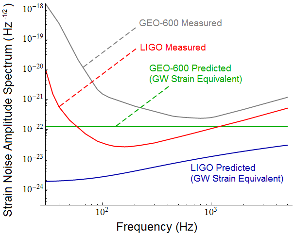
Figure 8: Spectra for holographic noise (baseline model), expressed as effective strain noise observed in gravitational wave interferometers. Published noise curves from LIGO and GEO-600 have been left in their original form to reflect sensitivity to gravitational wave strain. Predicted spectra for holographic noise have been converted into gravitational wave strain equivalents to demonstrate the levels observable in data published for gravitational wave strain. The predicted spectrum for GEO-600 is given by dividing eq. (47) by 2L and obtaining eq. (48), as the folded arm enhances gravitational wave sensitivity by an amplification factor of 2 that is not applicable to holographic noise. The spectrum for LIGO is given in eq. (54), where the spectrum in eq. (50) is divided by the amplification factor from Fabry-Perot cavities given in eq. (53). The flat strain amplitude for GEO-600, at $1.23\times 10^{-22}\textrm{Hz}^{-1/2}$, is consistent with the unidentified noise detected. The LIGO Scientific Collaboration (2011); The LIGO Scientific Collaboration and The Virgo Collaboration (2010); Frolov and Grote (2014)

We present the predicted and measured noise spectra from the baseline models in two different ways. Figure 7 shows the spectra plotted in terms of beam splitter position noise, relevant to measurements of Planckian directional entanglement. This figure displays all of the predicted spectra for holographic noise calculated in the previous section, and applies the previously calculated conversions to the noise spectra published by LIGO and GEO-600 in order to obtain the correct levels of sensitivity to this type of effect from noncommutative emergent spacetime.

Figure 8, on the other hand, presents everything in terms of equivalent levels of gravitational wave strain. Unlike the preceding plot, published noise curves from LIGO and GEO-600 are left unaltered. Instead of converting the published noise curves to reflect sensitivity to holographic noise, for this plot we have converted the predicted levels of holographic noise into gravitational wave strain equivalents to show what we expect to be measurable in experiments designed to detect gravitational wave strains coherently applied to folded light paths or Fabry-Perot cavities.

It should again be noted that the predicted holographic noise curves for LIGO are based on an effective model without a rigorous theory of how this Planckian directional entanglement would manifest in delocalized light modes within Fabry-Perot cavities. Hence the LIGO curves should be subject to some uncertainty in regions where the prediction based on probabilistic summation deviates from the reference curve for a simple Michelson configuration (see Figure 7). The prediction for GEO-600 is more quantitatively certain. But both predictions actually depend on our lengthy discussion in section III.2.2 being entirely correct about the nature of orthogonal interferometer arms as independent light clocks. It is possible that there are inaccuracies in our arguments about Hilbert space collapse. We should allow for the possibility that these estimates might be off by factors of 2 when determining the amplitude of transverse noise accumulated through the distances measured within the arms, or when adding the effects from the two arms in orthogonal directions. Still, these simple models allow a direct comparison of the various different configurations.

We have also omitted from our analysis any possible effect from the cavities created by signal recycling mirrors in GEO-600 or LIGO. While we expect the corrections necessary to be small, as our posited noise is fundamental to the spacetime itself, a more careful analysis is certainly due if any meaningful signal is detected in future experimental data.

The data from GEO-600 is of particular note, as it is the experiment closest to the sensitivity levels required to detect the effects of this hypothetical Planckian directional entanglement. Current sensitivity levelsFrolov and Grote (2014) are slightly better than the latest published levelsThe LIGO Scientific Collaboration (2011) used in the figures, by approximately 10-15% in strain amplitude at the lowest point. Sources of non-holographic environmental and technical noise are difficult to comprehensively identifyS. Hild for the GEO-600 Collaboration (2009), but the collaboration has developed a reliable model for shot noise and conducted a rough analysis of the frequency region where this is the only significant source of noise. At present, the data and model are consistent with unidentified flat-spectrum noise close to our baseline prediction of $1.23\times 10^{-22}\textrm{Hz}^{-1/2}$ in eq. (48) and Figure 8 Frolov and Grote (2014). Recent improvements in the sensitivity of the LIGO system are expected to bring its future noise spectra close to our predictions for holographic noise as well The LIGO Scientific Collaboration and The Virgo Collaboration (2016a). We conclude that holographic noise is not ruled out, but if it exists, should be measurable with a reasonable improvement in sensitivity or with the experimental design of the Holometer.

IV closing remarks

As noted previously, amongst the metric-based meta-models, LIGO data has made it clear that the “random walk” model with the flat measured noise spectrum cannot be valid, and indications are that the strain power spectrum of the spacetime noise cannot be independent of the physical scales of the measurement appartatus (the “white spacetime noise” model). The only simple theoretically motivated prediction that remains untested (albeit lacking in covariance) is the “one-third power” model.

These alternative models assume non-standard coherences that do not exist in field theory. Without those coherences, a simple field theoretic consideration shows that the interaction of a finite-width beam with the surface boundary conditions of a macroscopic object would average out the metric fluctuations in a way that would exponentially suppress the actually observable deviation in macroscopic distance. Experimental constraints also rule out the “one-third power” model in this case without macroscopic coherencePerlman et al. (2015).

The effective theory of position noise suggested by HoganHogan (2012a) posits a noncommutative spacetime and derives a Planckian random walk noise only in directions transverse to separation between bodies whose position is measured, over a time corresponding to that separation. The fluctuations in this case are not describable as perturbations of any metric, but are instead considered to be a result of a directionally entangled spacetime that emerges from overlapping causal diamonds amongst events and observers. Therefore more careful attention must be paid to the interferometer configuration to derive limits, by considering the phases of null waves whose interactions with matter define position operators. Our estimates show that the predicted level of noise is comparable to the unidentified noise observed in GEO-600, the detector most sensitive to this type of noise. The Holometer design should be able to reach a highly significant detection, or a constraining upper limit, by sampling data at high frequencies, and using two cross-correlated interferometers co-occupying the same space in order to average out uncorrelated high frequency shot noise over long integration times.