Faster graphical model identification of tandem mass spectra using peptide word lattices

Abstract

Liquid chromatography coupled with tandem mass spectrometry, also known as shotgun proteomics, is a widely-used high-throughput technology for identifying and quantifying proteins in complex biological samples. Analysis of the tens of thousands of fragmentation spectra produced by a typical shotgun proteomics experiment begins by assigning to each observed spectrum the peptide that is hypothesized to be responsible for generating the spectrum. This assignment is typically done by searching each spectrum against a database of peptides. We have recently described a machine learning method—Dynamic Bayesian Network for Rapid Identification of Peptides (DRIP)—that not only achieves state-of-the-art spectrum identification performance on a variety of datasets but also provides a trainable model capable of returning valuable auxiliary information regarding specific peptide-spectrum matches. In this work, we present two significant improvements to DRIP. First, we describe how to use word lattices, which are widely used in natural language processing, to significantly speed up DRIP’s computations. To our knowledge, all existing shotgun proteomics search engines compute independent scores between a given observed spectrum and each possible candidate peptide from the database. The key idea of the word lattice is to represent the set of candidate peptides in a single data structure, thereby allowing sharing of redundant computations among the different candidates. We demonstrate that using lattices in conjunction with DRIP leads to speedups on the order of tens across yeast and worm data sets. Second, we introduce a variant of DRIP that uses a discriminative training framework, performing maximum mutual entropy estimation rather than maximum likelihood estimation. This modification improves DRIP’s statistical power, enabling us to increase the number of identified spectrum at a 1% false discovery rate on yeast and worm data sets.

1 Introduction

The most widely used high-throughput technology to identify and quantify proteins in complex mixtures is shotgun proteomics, in which proteins are enzymatically digested, separated by micro-capillary liquid chromatography and subjected to two rounds of mass spectrometry. The primary output of a shotgun proteomics experiment is a collection of, typically, tens of thousands of fragmentation spectra, each of which ideally corresponds to a single generating peptide. The first, and arguably the most important, task in interpreting such data is to identify the peptide responsible for generating each observed spectrum.

The most accurate methods to solve this spectrum identification problem employ a database of peptides derived from the genome of the organism of interest (reviewed in [13]). Given an observed spectrum, peptides in the database are scored, and the top-scoring peptide is assigned to the spectrum. We recently proposed a machine learning method, called DRIP, that solves the spectrum identification problem using a dynamic Bayesian network (DBN) [4]. In this model, the “time” axis of the DBN corresponds to the mass-to-charge (m/z) axis of the observed spectrum. The model uses Viterbi decoding to align the observed spectrum to a theoretical spectrum derived from a given candidate peptide, while adjusting the corresponding score to account for insertions—a peak in the observed spectrum that is absent from the theoretical spectrum—and deletions—a peak in the theoretical spectrum that is absent from the observed spectrum. In DRIP, observed peaks are scored using Gaussians positioned along the m/z axis, the parameters of which are learned using a training set of high-confidence peptide-spectrum matches (PSMs). This approach allows the model to score observed spectra in their native resolution without quantization of the m/z axis.

The current work introduces DRIP to the computational biology community and describes several important improvements to the method.

• First, and most significantly, we describe how to use word lattices [7] to make DRIP more efficient. Word lattices are widely used in natural language processing to jointly represent a large collection of natural language strings. In the context of shotgun proteomics, a word lattice can be used to represent compactly the collection of candidate peptides (i.e., peptides whose masses are close to the precursor mass) associated with an observed fragmentation spectrum. Using the lattice during Viterbi decoding allows for the sharing of computation relative to the different candidate peptides. Without loss of performance, the lattice approach provides a significant reduction in computational expense, ranging from 85–93% in the yeast and worm data sets that we examine here. Notably, this general approach to sharing computations among candidate peptides is generally applicable to any scoring function that can be framed as a dynamic programming operation.

• Second, facilitated by the incorporation of word lattices, we extend DRIP’s learning framework to use discriminative training. Thus, rather than performing maximum likelihood estimation on a training set of high-confidence PSMs, DRIP performs maximum mutual information estimation to discriminate between the high-confidence PSMs and a large “background” collection of candidate PSMs. Empirical evidence suggests that this discriminative approach provides an improvement in statistical power relative to the generatively trained version of DRIP.

• Third, we introduce several improvements to the model, including removing the need to specify several hyperparameters (maximum number of allowed insertions and deletions per match) a priori and a calibration procedure to allow joint ranking of PSMs with different charge states.

The final DRIP model provides an efficient and accurate method for assigning peptides to observed fragmentation spectra from a shotgun proteomics experiment, all implemented within a rigorously probabilistic and easily extensible modeling paradigm.

2 Overview of Tandem Mass Spectrometry

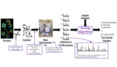
Figure 1: A typical shotgun proteomics experiment.

A typical shotgun proteomics experiment (Figure 1) begins by cleaving proteins into peptides using a digesting enzyme, such as trypsin. The resulting peptides are then separated via liquid chromatography and injected into the mass spectrometer. In the first round of mass spectrometry, the mass and charge of the intact precursor peptide are measured. Peptides are then fragmented, and the fragments undergo a second round of mass spectrometry. The intensity of each observed peak in the resulting fragmentation spectrum is roughly proportional to the abundance of a single fragment ion with a particular m/z value.

Formally, we can represent the spectrum identification problem as follows. Let $\mathcal{P}$ be the set of all possible peptide sequences. Given an oberved spectrum $s$ with precursor mass $m^{s}$ and precursor charge $c^{s}$, and given a database of peptides $\mathcal{D}\subseteq\mathcal{P}$, we wish to find the peptide $x\in\mathcal{D}$ responsible for generating $s$. Using the precursor mass and charge, we may constrain the set of peptides to be scored by setting a mass tolerance threshold, $w$, such that we score the set of candidate peptides

$$D(m^{s},c^{s},\mathcal{D},w)=\left\{x:x\in\mathcal{D},\,\left|\frac{m(x)}{c^{s}}-m^{s}\right|\leq w\right\},$$ (1)

where $m(x)$ denotes the mass of peptide $x$. Denoting an arbitrary scoring function as $\psi(x,s)$, the spectrum identification problem requires finding

$$x^{*}=\operatorname*{argmax}_{x\in D(m^{s},c^{s},\mathcal{D},w)}\psi(x,s).$$ (2)

3 Benchmark methods

To score a peptide $x$ with respect to a spectrum $s$, most scoring algorithms first construct a theoretical spectrum comprised of the peptide’s expected fragment ions. Denoting the length of $x$ as $n$ and, for convenience, letting $\tilde{n}=n-1$, $x=x_{0}x_{1}\dots x_{\tilde{n}}$ is a string. The fragment ions of $x$ are shifted prefix and suffix sums called b- and y-ions, respectively. Denoting these two as functions $b(\cdot,\cdot,\cdot),y(\cdot,\cdot,\cdot)$, we have

$$b(x,c^{b},k)=\mbox{round}\left(\frac{\sum_{i=0}^{k-1}m(x_{i})+c^{b}}{c^{b}}\right), y(x,c^{y},k)=\mbox{round}\left(\frac{\sum_{i=\tilde{n}-k}^{\tilde{n}}m(x_{i})+18+c^{y}}{c^{y}}\right),$$ (3)

where $c^{b}$ and $c^{y}$ are charges related to the precursor charge state. The b-ion offset corresponds to the mass of a $c^{b}$ charged hydrogen atom, while the y-ion offset corresponds to the mass of a water molecule plus a $c^{y}$ charged hydrogen atom. When $c^{s}\in\{1,2\}$, $c^{b}$ and $c^{y}$ are unity because, for any b- and y-ion pair, an ion with no charge is undetectable in the mass spectrometer and it is unlikely for both charges in a +2 charged precursor ion to end up on a single fragment ion. When $c^{s}\geq 3$, we search both singly and doubly charged ions so that $c^{b},c^{y}\in\{1,2\}$. Denoting the number of unique b- and y-ions as $n^{x}$ and, for convenience, letting $\widetilde{n}^{x}=n^{x}-1$, our theoretical spectrum is thus a sorted vector $v^{x}=(v_{0},\dots,v_{\widetilde{n}^{x}})$ consisting of the unique b- and y-ions of $x$.

We benchmark DRIP’s performance relative to four widely used search algorithms. The score function used by the first such algorithm, MS-GF+ [10], is a scalar product between a heavily preprocessed observed spectrum, $\tilde{s}$, and a binary theoretical vector of equal length, $u$. MS-GF+ then ranks all the candidate peptides for a given spectrum by calculating the p-value of $u^{T}\tilde{s}$ over a distribution of scores for all peptides with equal precursor mass. Although the number of distinct peptide sequences with masses close to the observed precursor mass is large (on the order of $10^{20}$ in many cases), the linearity of $u^{T}\tilde{s}$ allows the full distribution of scores of all such peptides to be computed efficiently using dynamic programming. MS-GF+ version 9980 was used, and the E-value score was used for scoring of spectra.

The remaining three benchmark algorithms are variants of SEQUEST [2], each implemented in Crux v2.1 [12]. Like MS-GF+, the SEQUEST algorithm begins by quantizing and preprocessing the observed spectrum into a vector, $\tilde{s}$. A vector of equal length, $u$, is constructed based on the theoretical spectrum, and XCorr takes the form

$$\mbox{XCorr}(s,x)=\tilde{u}^{T}\tilde{s}-\frac{1}{151}\sum_{\tau=-75}^{75}\tilde{u}^{T}\tilde{s}_{\tau}=\tilde{u}^{T}(\tilde{s}-\frac{1}{151}\sum_{\tau=-75}^{75}\tilde{s}_{\tau})=\tilde{u}^{T}\tilde{s}^{\prime},$$ (4)

where $\tilde{s}_{\tau}$ denotes the vector shifted by $\tau$ m/z units. Thus, XCorr is a foreground (scalar product) minus a background score. We report results from (1) the XCorr score as implemented in Tide [1], (2) the XCorr E-value computed by Comet [3] by fitting, for each spectrum, an exponential distribution to the candidate peptide XCorr scores, and (3) the XCorr p-value computed by Tide using a dynamic programming approach similar to that used by MS-GF+ [6].

4 Dynamic Bayesian Network for Rapid Identification of Peptides (DRIP)

A graphical model is a formal representation of the factorization of the joint distribution governing a set of random variables via a graph, the nodes of which denote random variables and the edges of which denote potential conditional dependence between nodes . This formalization enables a host of tractable inference algorithms while offering incredible modeling flexibility. A Bayesian network is a graphical model defined over directed acyclic graphs, and a dynamic Bayesian network (DBN) is a Bayeian network defined over variable length temporal sequences. The basic time unit of a DBN, determined by the time units of the temporal process being modeled, is called a frame and consists of a group of nodes and edges amongst these nodes. A DBN is often defined in terms of a template, where the first and last frame are called the prologue and emphepiloque, respectively, and where the chunk is expanded to occupy all frames in between. The template of DRIP is depicted in Figure 2.

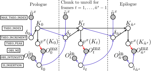
Figure 2: Graph of DRIP.

The DRIP model itself represents the observed spectrum, and each frame in DRIP corresponds to a single observed peak. The theoretical spectrum is hidden and traversed from left to right as follows. Denoting the number of frames as $n^{s}$ and, for convenience, letting $\widetilde{n}^{s}=n^{s}-1$ and $t$ be an aribtrary frame $0\leq t\leq\widetilde{n}^{s}$, $K_{t}$ denotes the index of the current theoretical peak, which is a deterministic function of its parents such that $K_{0}=\delta_{0}$ and $K_{t}=K_{t-1}+\delta_{t}$ for $t>0$, where $\delta_{t}$ is a multinomial random variable. Thus, $\delta_{t}$ denotes the number of theoretical peaks we traverse in subsequent frames. Furthermore, the parents of $\delta_{t}$, $\widetilde{n}^{x}$ and $K_{t-1}$, constrain it from being larger than the number of remaining theoretical peaks left to traverse. $v^{x}(K_{t})$ is thus the $K_{t}$th theoretical peak. The variables $O^{\mbox{mz}}_{t}$ and $O^{\mbox{in}}_{t}$ are the observed m/z and intensity values, respectively, of the $t$th observed peak, where $O^{\mbox{mz}}_{t}$ is scored using a Gaussian centered near $v^{x}(K_{t})$ and $O^{\mbox{in}}_{t}$ is scored using a Gaussian whose learned variance is larger than that of the m/z Gaussians, thus prioritizing matching well along the m/z axis as opposed to high-intensity peaks. Parent to these observed variables is $i_{t}$, a Bernoulli random variable which denotes whether an observed peak is considered an insertion, $i_{t}=1$, or not. When $i_{t}=1$, a constant penalty is returned rather than scoring the observed observations with the currently considered Gaussians dictated by $K_{t}$, since scores may become arbitrarily bad by allowing Gaussians to score m/z observations far from their means and this would make the comparability of scores impossible (a single insertion would make an otherwise great alignment terrible). Furthermore, so as to enforce that some observations be scored rather than inserted, $i_{t}$ enforces its child $\delta_{t+1}$ to be zero in a frame following an insertion. Because $\delta_{t}$ and $i_{t}$ are hidden, DRIP considers all possible alignments, i.e., all possible combinations of insertions and theoretical peaks scoring observed peaks. The Viterbi path, i.e., the alignment which maximizes the log-likelihood of all the random variables, is used to score a peptide as well determine which observed peaks are most likely insertions and which theoretical peaks are most likely deletions.

Note that the version of DRIP used in this work (Figure 2) is somewhat simplified relative to the previously described DRIP model [4]. In particular, the previously described version of DRIP required two user-specified quantities, corresponding to the maximum allowable numbers of insertions and deletions. These constraints were enforced via two chains of variables, which kept track of the number of utilized insertions and deletions in an alignment, counting down in subsequent frames. The current, simplified model automatically determines these two quantities on the basis of the deletion and insertion probabilities as well as the insertion penalties. This simplification comes at no detriment to performance or running time (data not shown).

4.1 Calibrating DRIP with respect to charge

For observed fragmentation spectra with low-resolution precursor data often have indeterminate charge states. For such spectra, all candidates are scored and ranked assuming all charge states, with the highest scoring peptide amongst all charges returned. This approach requires that scores among differently charged spectra be comparable to one another. In DRIP, however, this is not the case. Because the number of theoretical peaks essentially doubles when moving from charge 2+ to charge 3+, higher charged PSMs which have denser theoretical spectra and thus much better scores than lower charged PSMs, rendering differently charged PSMs incomparable.

In order to alleviate this problem, we recalibrate scores on a per charge basis, projecting differently charged PSM scores to roughly the same range. The procedure consists of first generating a secondary set of decoy peptides disjoint from the target peptide set and primary decoy peptide sets. Let $\mathcal{D}^{t}$ be the set of target peptides, $\mathcal{D}^{d}$ be the set of decoy peptides, and $\mathcal{D}^{dd}$ be our new set of decoy peptides, such that $\mathcal{D}^{dd}\cap(\mathcal{D}^{t}\cup\mathcal{D}^{d})=\emptyset$. Next, all spectra and charge states are searched, returning top ranking sets of PSMs $\mathcal{X}^{t}\subseteq\mathcal{D}^{t}$, $\mathcal{X}^{d}\subseteq\mathcal{D}^{d}$, and $\mathcal{X}^{dd}\subseteq\mathcal{D}^{dd}$. We then partition $\mathcal{X}^{dd}$ based on charge. For each charge $c$ and corresponding partition, $\mathcal{Z}^{dd}$, we rank all PSMs based on score. Let $\mathcal{Z}^{t}\subseteq\mathcal{X}^{t}$ be all PSMs of charge $c$, for which we use their scores to linearly interpolate their normalized ranks in $\mathcal{Z}^{dd}$, using these interpolated normalized ranks as their new calibrated scores. In order to recalibrate scores greater than those found in $\mathcal{Z}^{dd}$, we use the 99.99th percentile score and maximal score for linear interpolation. Once this procedure is done, a majority of recalibrated scores for PSMs in $\mathcal{Z}^{t}$ and $\mathcal{Z}^{d}$ will lie between $[0,1]$ and a few barely above unity(this is largely true for the targets, since a set of well expressed and identifiable target peptides typically outscores all decoys), thus greatly decreasing the dynamic range of scores. With these recalibrated scores, we may easily take the top ranking PSM of an observed spectrum amongst differently charged PSMs, without any loss in overall accuracy.

5 Word Lattices

Word lattices (abbreviated as lattices for this section) represent data instances compactly in graphical structures and have gained great success in the fields of natural language processing and speech recognition. For example, natural language dictionaries can be stored in lattices for more efficient querying; in speech recognition, lattices constructed out of the top phone/word level hypotheses can be used to rescore and select the best hypothesis effectively.

A lattice over an alphabet $\Sigma$ is a directed graph $G=(N,E,s,t)$, where $N$ is the node set, $E$ is the edge set, and $s,t\in N$ denote the source and target node respectively. Every edge $e\in E$ is a tuple $(n_{1},n_{2},\alpha(e))$, where $n_{1},n_{2}$ are the from-node and to-node respectively, and $\alpha(e)\in\Sigma$ is the alphabet element encoded in $e$.

A lattice encodes data on paths from $s$ to $t$. Let $P(G,s,t)$ denote the set of paths from $s$ to $t$, then every $p=e_{1},e_{2},..,e_{|p|}$, $p\in P(G,s,t)$ represents a sequence of characters, or a string, over alphabet $\Sigma$: $\alpha(e_{1}),\alpha(e_{2}),..,\alpha(e_{|p|})$. For notation simplicity, let $P(G,e_{1},e_{2})$, where $e_{1},e_{2}\ inE$, denote the set of paths starting in $e_{1}$ and ending in $e_{2}$.

An alternative way to define a lattice is to consider it as a nondeterministic finite automaton (NFA) $G=(Q,\Sigma,\Delta,q_{0},F)$, where $Q$ denotes the set of states, which is equivalent to the node set in the directed graph definition, $\Delta$ is the transition function: $Q\times\Sigma\rightarrow 2^{Q}$, $q_{0}$ is the initial state and $F=\{f\}$ is the final state. $q_{0}$ and $f$ correspond to $s,t$ in the directed graph definition respectively. The NFA definition is useful when we consider the problem of constructing a lattice from a set of strings.

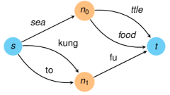
Figure 3: An Example Lattice: encodes “seattle”, “’seafood’, “kungfu”, and “tofu”; the alphabet can be any string over [a-z] of length $\leq 4$.

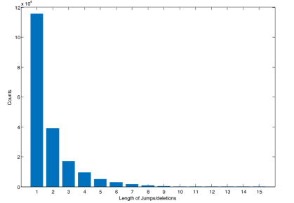
Figure 4: Jump Histogram

Suppose we are given a set of strings $X=\{x_{1},x_{2},...,x_{m}\}$. The lattice representation of the strings $G(X)$ can be extremely compressed as there may be significant amount of redundant information shared among elements of $X$. More specifically, if $x_{i}$ and $x_{j}$ share some substring in common, we can merge the shared parts into a sequence of common edges, instead of representing the same substring twice. Fig. 4 gives a lattice over four word strings, with the shared substrings collapsed into common edges to reduce the redundancy.

The common edges of lattices not only save space for data representation, but also speed-up complex operations using the encoded data. For this paper in particular, we focus on the task of dynamic graphical model inference with Viterbi algorithm. With lattices, we manage to both reduce the state space of Viterbi algorithm, and apply smart pruning strategies in a more effective way, as we will discuss in details later, which result in magnitudes of speed-ups.

5.1 Lattice Construction

To construct the optimal lattice from input set of strings $X$ over alphabet $\Sigma$ is a hard problem. The objective of the “optimal” lattice is task dependent. E.g., for dictionary queries, the optimal lattice should have the minimal number of nodes/states, which correspond to the major computation time; for data compression, the optimal lattice should be minimal in overall size, in which case both the nodes and edges matter. Moreover, some tasks do not require the lattice to be an “exact” representation of the input strings. For a set of strings $X$, an exact lattice is an NFA that accepts only language $\mathbb{L}(G(x))=X$. For our task, which is to speed-up graphical model training/inference, we choose the objective to be: construct lattice $G(X)=(N,E,s,t)$ such that $G(X)$ is exact and $|E|$ is minimized.

As stated above, we can think a lattice as an NFA, and it has been proven that NFA minimization in terms of number of states/transitions are NP-hard to approximate within constant factors. To approximate the optimal lattice, we give the following algorithm which is similar to the determinize-minimize algorithm of minimizing a DFA[14]. The result lattice $G(X)$ is the minimum state DFA of the same language $X$.

Algorithm 1 $ConstructLattice(X,\Sigma)$

1:$G=\{\{s,t\},\emptyset,s,t\}$.

2:Assign an ordering in $\Sigma$, and sort $X$.

3:for $x\in X$ do

4:    Start from $s$, traverse $G$ with $x$. Stop when no matching edge can be found: suppose the non-matching character is $x[i]$, and we stop at node $n^{\prime}$.

5:    Build a chain structure $C$ out of $x[i:]$, where each edge on the chain corresponds to one character.

6:    Merge $C$ into $G$ by merging the start node of $C$ with $n^{\prime}$ and the end node of $C$ with $t$.

7:end for

8:Run DFA minimization on $G$.

9:return $G$.

The for loop, which merges prefixes of input strings, constructs a DFA out of $X$. Minimization on the constructed DFA can be thought as a process that merges nodes, which share the same suffixes. Both merging prefixes and suffixes reduce the number of edges in the lattice, making the algorithm a powerful heuristic in practice, and managing to reduce up to 50% edges as we will show in the result section. The complexity of the algorithm is bounded by the DFA minimization step. With Hopcroft’s algorithm [5], the running time is $\mathcal{O}(|\Sigma||X|l_{\max}log(|X|l_{\max}))$, where $l_{\max}=\max_{x\in X}|x|$.

5.2 Representation of Lattices in Dynamic Graphical Models

We can utilize dynamic graphical model structures to naturally traverse a lattice $G$ to access the encoded data. Particularly, for time frame $t$, we use three vertices to access the lattice: the lattice node vertex $V_{t}$, the lattice link vertex $L_{t}$, and the transition vertex $T_{t}$. $V_{t}$’s and $T_{t}$’s decide the set of values that $L_{t}$’s can take on, and each value of $L_{t}$ corresponds to one character in the encoded strings.

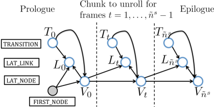
Figure 5: Representation of Lattices in Dynamic Graphical Models

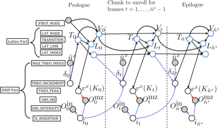
Figure 6: Lattice DRIP Model

Fig. 6 shows the lattice representaion as dynamic graphical model structures. $V_{t}=n_{i}$, $T_{t+1}=d$ ($d\geq 0$) determines the set of nodes $V_{t+1}$ can take: $V_{t+1}=\{n_{j}\in N\mbox{ }|\exists p\in P(G,n_{i},n_{j}),|p|=d\}$. $V_{t}=n_{i}$, $V_{t+1}=n_{j}$, and $T_{t+1}=d$, together determines the set of edges $L_{t+1}=\{e\in E\mbox{ }|p\in P(G,n_{i},n_{j}),|p|=d,p[d-1]=e\}$. In another word, $L_{t+1}$ is a random variable corresponding to all edges that go into $n_{j}$ and can be reached from $n_{i}$ with a path of length $d$. For the simple case, we may enforce $T_{t}\in\{0,1\}$. If $T_{t}=0$, we stay at the current node, and if $T_{t+1}=1$, $L_{t+1}$ becomes the set of outgoing edges from $n_{i}$, and $V_{t+1}$ becomes the set of destination nodes of the outgoing edges. “FIRST_NODE” vertex has the observatoin of the source node value $s$, and is used for initializing the time dependent structure.

The complexity for constructing the deterministic conditional probability table (CPT), which stores $Pr(L_{t}|V_{t},V_{t+1},T_{t+1})$, for traversing the lattice as stated above is $|\{(e_{1},e_{2})\mbox{ }|e_{1},e_{2}\in E,\exists p\in P(G,e_{1},e_{2}),|p|\leq d_{\max}\}|$, where $d_{\max}$ is the largest value $T_{t}$ can take, or in another word, maximum number of edges to “jump over”. Please note that the CPT can be very sparse depending on the structure of the lattice as there may not exist a path between two nodes $n_{i}$ and $n_{j}$. The value of $d_{\max}$ can vary based on the underlying graphical model. If only edge-by-edge traversal of the lattice is required, than $d_{\max}=1$. For DRIP, which we will talk in details later, $d_{\max}=\max_{x\in X}|x|$, which is the length of the longest candidate peptide. However, we may constrain $d_{\max}$ to take much smaller value than $\max_{x\in X}|x|$, as such long jumps are very unlikely in probability, so that we trade-off significant speed-ups with negligible performance loss.

Please note that the representation of lattices in GM can suit for any underlying dynamic graphical models, which access data in a streaming-like manner (do not go back and access previous data). Rather than accessing data in the traditional way, the lattice representation brings two major benefits: 1) various pruning strategies can be applied to speed-up the underlying GM significantly; 2) such compressed representation enables possibility of certain expensive learning methods, which requires to access the entire set of data, such as discriminative training.

5.3 Lattice with DRIP

Naturally, we convert the input of DRIP, which is a set of theoretical peptide peaks $v^{x}$ within certain mass window around the precursor mass, into a peptide peak lattice $G_{p}$. The alphabet $\Sigma_{p}$ for $G_{p}$ contains all possible peak m/z values (in Daltons) rounded to the nearest integer values. We build a lattice for each set of peptide candidates within certain mass window. The lattices then become the “database” to search for the best peptide candidate match. We don’t count lattice construction time as an overhead as we can reuse the lattices for future queries just like a database.

Fig .6 shows the complete graphical model for Lattice DRIP. The “THEO_INCREMENT” vertex $\delta_{t}$, which controls the number of deletions in DRIP, behaves similarly as the transition random variable $T_{t}$ in the lattice representation in GM, and we feed the value of $\delta_{t}$ into $T_{t}$. “LAT_INDEX” keeps track of the number of edges from the current node to $s$. At first frame, the max value $T_{0}$ can take is then the max value of $\delta_{t}$, which is capped at $\max_{x\in X}|x|$. Over time frames, the max value of $T_{t}$ decreases as the rest lengths of peptides decrease. Different from the original DRIP model, where the rest length of each peptide candidate can be specified exactly, as only one peptide is process as a time, it is hard to map from the set of edges traversed so far to one specific peptide candidate, for the reason that multiple peptides can share those set of edges. As an approximation, we choose to use the rest length of the longest peptide encoded in the lattice as the rest lengths for all peptides. Theoretically, the Lattice DRIP score of a peptide would be a lower bound on the peptide’s original DRIP score, as $Pr(\delta_{t}=a|\max(\delta_{t})=b)<Pr(\delta_{t}=a|\max(\delta_{t})=c)$ if $b>c>a$. In practice, we find such effect negligible, as we will show in the result session.

The value of $L_{t}$, which contains the set of m/z values of b/y-ions, is fed into the “THEO_PEAK” vertex $v^{x}(K_{t})$ for scoring based on the mean Gaussians and the intensity Gaussian. The lattice acts like a “database” for querying theoretical peaks, and it does not affect the mechanism of the underlying GM.

5.4 Speeding Up Graphical Models with Lattices

Lattices are compressed representations of the encoded data instances. By applying lattices in graphical models, the state space for accessing all the data instances is smaller compared to the original case where each data instance is accessed separately. An intuitive illustration is to consider about the “simple lattice”, which contains $|X|$ disjoint paths from $s$ to $t$, and each path corresponds to one data instance. The state space for the simple lattice is no different from accessing each data instance separately. By constructing the lattice, common structures in the simple lattice get merged into shared edges so that the state space is smaller. Depending on the input data instances, the state space reduction can be significant. As data gets larger, we would expect more shared structures, so that the sizes of lattices grow only sublinearly. For the task of mass spectrometry, there are often hundreds of candidate peptides within a certain mass window for one spectrum, out of which around up to 50% of peaks can be identified as redundant by the lattices. PTMs and other modifications to the peptides may enlarge the number of candidates to search tremendously, where lattices can perform more efficiently.

Beam pruning, which is a heuristic algorithm that expands only a pruned set of hypotheses in graphical model inference, fit perfectly with lattices. Different beam pruning strategies such as k-beam pruning, which preserves only k hypothesis states at each time frame $t$, shrinks the state space of graphical model inference significantly. The hypothesis states of the original DRIP only consist of various deletion/insertion sequences of a single peptide candidate. Therefore, when various beam pruning strategies are applied, bad deletion/insertion sequences of the peptide get pruned away, yet we still end up evaluating every peptide candidate even though the best deletion/insertion sequences of certain peptides don’t match the spectrum well. With lattices, beam pruning methods force peptide candidates filter themselves collaboratively. When applying beam pruning methods with lattices, the state space consists of various deletion/insertion sequences of all the peptide candidates. The badly scored peptides get pruned early on, and we end up scoring only a subset of the candidates.

Reduce the maximum value of $T_{t}$ also decreases the search space of lattice. As stated above, complexity of the lattice traversing deterministic CPT is $|\{(e_{1},e_{2})\mbox{ }|e_{1},e_{2}\in E,\exists p\in P(G,e_{1},e_{2}),|p|\leq d_{\max}\}|$. For DRIP, longer “jumps” or deletions are attributed with smaller probabilities. From Fig. 4, which depicts the histogram of the length of deletions, long jumps are unlikely for the best-matching candidate. Therefore, the maximum value of $T_{t}$ can be set small, and rarely do we lose any good candidate. In practice, for Lattice DRIP we set the maximum allowed value of $T_{t}$ to 20.

There are enormous other ways to prune the lattices to accelerate the graphical model inference thanks to the lattices’ capability of identifying common structures within the data. Pruning lattices statically like pruning trees, as well as embed probabilities into lattice edges to get pruning subject to certain distributions, may achieve good speed-ups, while the beam pruning and the limit of the longest jump, as we will mention in the result section, have gained us 7 to 15 times of acceleration.

6 Training DRIP

DRIP is a highly trainable model amenable to learning its Gaussian parameters, which provides both a tool to explore the nonlinear m/z offsets caused by machine error as well as a significant boost in performance. For the overall training procedure, assume that we have a collection, $C$, of $N$ i.i.d. pairs $(s^{i},x^{i})$, where $s^{i}$ is an observed spectrum and $x^{i}$ the corresponding PSM we have strong evidence to believe generated $s^{i}$. Let $\theta$ be the set of parameters for which we would like to learn, in our case DRIP’s Gaussian parameters. For generative training, we then wish to find $\theta^{*}=\operatorname*{argmax}_{\theta}\sum_{i=1}^{N}p(s^{i}|x^{i},\theta)$, i.e. we wish to maximize DRIP’s likelihood with respect to the parameters to be learned, achieved via expectation-maximization (EM).

A much more difficult training paradigm is that of discriminative training, wherein we do not simply wish to maximize the likelihood under a set of parameters, but we would also like to simultaneously minimize a parameterized distribution defined over a set of alternative hypotheses. In our case, this alternative set of hypotheses consists of all candidate peptides within the precursor mass tolerance not equal to $x^{i}$, i.e. all incorrect explanations of $s^{i}$. More formally, our discriminative training criterion is that of Maximum Mutual Information Estimation (MMIE); defining the set of candidate peptides for $s^{i}$ within precursor mass tolerance $w$ as $\mathcal{C}^{i}=D(m^{s},c^{s},\mathcal{D},w)$ and denoting the set of all training spectra and high-confidence PSMs as $\mathcal{S}$ and $\mathcal{X}$, respectively, the function we would like to maximize with respect to $\theta$ is then

$$I_{\theta}(\mathcal{S};\mathcal{X}) = \mathbb{E}\log\frac{p(s^{i},x^{i}|\theta)}{p(s^{i}|\theta)p(x^{i}|\theta)}=\sum_{s^{i},\mathcal{C}^{i}}p(s^{i},\mathcal{C}^{i}|\theta)\log\frac{p(s^{i},x^{i}|\theta)}{p(s^{i}|\theta)p(x^{i}|\theta)}=\sum_{s^{i},\mathcal{C}^{i}}p(s^{i},\mathcal{C}^{i}|\theta)\log\frac{p(s^{i}|x^{i},\theta)p(x^{i}|\theta)}{p(s^{i}|\theta)p(x^{i}|\theta)}$$ (5)

$$= \sum_{s^{i},\mathcal{C}^{i}}p(s^{i},\mathcal{C}^{i}|\theta)\log\frac{p(s^{i}|x^{i},\theta)}{p(s^{i}|\theta)}=\sum_{s^{i},\mathcal{C}^{i}}p(s^{i},\mathcal{C}^{i}|\theta)\log\frac{p(s^{i}|x^{i},\theta)}{\sum_{x\in\mathcal{C}^{i}}p(s^{i},x|\theta)}.$$

We approximate this objective using the quantity $\tilde{I}_{\theta}(\mathcal{S};\mathcal{X})=\frac{1}{N}\sum_{i=1}^{N}\log\frac{p(s^{i}|x^{i},\theta)}{\sum_{x\in\mathcal{C}^{i}}p(s^{i},x|\theta)}$, which converges to the quantity in Equation 5 for large $N$ by the i.i.d. assumption and the weak law of large numbers. Our objective is then

$$\max_{\theta}\tilde{I}_{\theta}(\mathcal{S};\mathcal{X}) = \max_{\theta}\frac{1}{N}\sum_{i=1}^{N}\log\frac{p(s^{i}|x^{i},\theta)}{\sum_{x\in\mathcal{C}^{i}}p(s^{i},x|\theta)}=\max_{\theta}\frac{1}{N}\sum_{i=1}^{N}\left(\log p(s^{i}|x^{i},\theta)-\log\sum_{x\in\mathcal{C}^{i}}p(s^{i},x|\theta)\right),$$ (6)

where, for obvious reasons, we call $M_{n}(s^{i},x^{i})=\log p(s^{i}|x^{i},\theta)$ the numerator model and $M_{d}(x^{i})=\log\sum_{x\in\mathcal{C}^{i}}p(s^{i},x|\theta)$ the denominator model. Note that the numerator model is our objective function for generative training, and in general the sum over possible peptide candidates in the denominator model makes the discriminative training objective difficult to compute. However, by using lattices to efficiently perform the computation in the denominator model, we solve Equation 6 using stochastic gradient ascent.

In stochastic gradient ascent, we calculate the gradient of the objective function with regard to a single training instance,

$$\nabla_{\theta}\tilde{I}_{\theta}(s^{i};x^{i}) = \nabla_{\theta}M_{n}(s^{i}|x^{i}\theta)-\nabla_{\theta}M_{d}(s^{i}|\theta),$$ (7)

where the gradients of $M_{n}$ and $M_{d}$ are vectors referred to as Fisher scores. Correspondingly, we update the parameters $\theta$ using the previous parameters plus a damped version of Equation 7, iterating this process until convergence. The overall algorithm is detailed in Algorithm 2. In practice, we begin the algorithm by initializing $\theta_{0}$ to a good initial value, i.e. the output of generative training, and the learning rate $\eta_{j}$ is updated with $\eta_{j+1}=(\sqrt{j})^{-1}$. Intuitively, the gradients move in the direction maximizing the difference between the numerator and denominator models, encouraging improvement for the numerator while discriminating against the incorrect labels in the denominator. Our experimental results show that discriminative training positively influences performance (Section 8.3).

Algorithm 2 Discriminative Training via Stochastic Gradient Ascent

1:Initialize $\theta_{0}$, $\eta_{0}$. Let $j=0$.

2:while True do

3:    $\theta_{j+1}:=\theta_{j}$; $j:=j+1$;

4:    Update learning rate $\eta_{j}$;

5:    for $(s^{i},x^{i})\in C$ do

6:       $\theta_{j}:=\theta_{j}+\eta_{j}(\nabla_{\theta}M_{n}(s^{i})|x^{i}\theta)-\nabla_{\theta}M_{d}(s^{i}|\theta))$;

7:    end for

8:    if $||\frac{\theta_{j}-\theta_{j-1}}{\theta_{j-1}}||<\epsilon$ then

9:       break;

10:    end if

11:end while

6.1 Discriminative Training with Lattices

Discriminative training is expensive to execute. The denominator model requires calculating the gradients of all possible candidate peptides $\mathcal{C}^{i}$, which can be infeasible for many tasks, yet to represent all possible labels in some graphical models, e.g. DRIP, is neither a trivial task. The hardness of representing all possible labels in DRIP comes from the fact that it is difficult to constrain the model to consider valid peptides only, as the distance between subsequent theoretical peaks can take on any value.

Lattices work perfectly with discriminative training in solving the scalability and representability problem. The lattice of all possible labels can be very compact, together with different strategies to speed up graphical model with lattices discussed in the previous session, discriminative training with lattice can be quite feasible and efficient.

The Lattice is a general framework to represent hypotheses for any dynamic graphical model. The denominator model of the discriminative training for DRIP is exactly the same as the Lattice DRIP model. Even for graphical models, which are capable of encoding all possible labels for discriminative training, lattices have the advantage of being more efficient and amenable to various modifications, as we can encode any set of labels into the lattice, so that discriminative training against any distribution is achievable.

7 Experimental methods

We benchmark all methods using three data sets: one low-resolution data set from the yeast S. cerevisiae consisting of 35,236 spectra (Yeast), one low-resolution data set from C. elegans consisting of 23,697 spectra (Worm-I), and one high-resolution C. elegans dataset consisting of 7,557 spectra (Worm-II). Further details regarding the Yeast and Worm-I datasets and corresponding target databases may be found in [8], and details regarding Worm-II and its database may be found in [6]. The datasets and target databases are available on the corresponding supplementary pages.

In order to ensure that all methods score exactly the same peptides, each search engine was provided with a pre-digested set of peptide sequences, rather than intact proteins sequences. Each protein database was digested using trypsin without suppression of cleavage by proline. Precursor charges range from 1+ to 3+ for Worm-I and Yeast and from 1+ to 5+ for Worm-II. For spectra with multiple charge states, the top scoring PSM was chosen per method.

All search algorithms were run with as equivalent settings as possible; machines were specified to CID, no allowance for missed cleavages or isotope errors, and a single fixed carbamidomethyl modification. For the two data sets with low-resolution precursors (Yeast and Worm-I), the mass tolerance $w$ was set to $\pm$ 3 Th, whereas for Worm-II $w$ was set to $\pm$ 10 ppm. Comet searches (XCorr E-values) used flanking peaks around each b- and y-ion, whereas Tide searches (XCorr and XCorr p-values) did not. These settings provided optimal performance for the two methods. All benchmark methods included neutral loss peaks in theoretical spectra, although these peaks are not modeled in DRIP.

A significant challenge in evaluating the quality of a spectrum identification algorithm is the absence of a “ground truth” data set where the generating spectrum is known for each observed spectrum. We therefore follow the standard approach of using decoy peptides (which in our case correspond to randomly shuffled versions of each real target peptide) to estimate the number of incorrect identifications in a given set of identified spectra. In this work, targets and decoys are scored separately and used to estimate the number of identified matches at a particular false discovery rate (FDR), i.e. the fraction of spectra improperly identified at a given significance threshold [9]. Because the FDR is not monotonic with respect to the underlying score, we instead use the q-value, defined to be the minimum FDR threshold at which a given score is deemed to be significant. Since data sets containing more than 10% incorrect identifications are generally not practically useful, we only plot $q$-values in the range $[0,0.1]$.

8 Results

8.1 Charge calibration improves statistical power

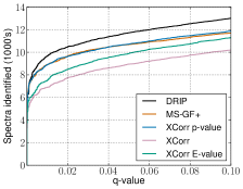
(a) Worm-I

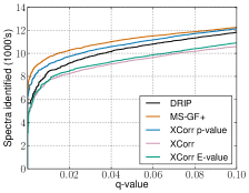
(b) Yeast

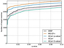
(c) Worm-II

Figure 7: Charge variation results for all datasets.

DRIP charge recalibrated outperforms XCorr and XCorr E-value on all datasets, and outperforms all datasets on Worm-I by a large margin. Though DRIP is outperformed by the two p-value methods on Yeast-I and Worm-II, this gap may be closed by gathering training data better representative of the corresponding spectra and their charge states (the high quality training data used only contains charge 2+ PSMs), which is currently underway. Furthermore, with the incorporation of lattices into DRIP, we now have a mechanism by which to sequence through entire sets of peptides. We believe this to be a critical step towards evaluating DRIP score thresholds with respect to arbitrary peptide sets, thus allowing the computation of DRIP p-values for which a performance increase such as XCorr to XCorr p-value is expected. It is worth noting that while MS-GF+ and XCorr p-value evaluate the entire set of possible peptides equal to a given precursor mass, the utilization of lattices allows DRIP to evaluate an arbitrary set of peptides (even regardless of precursor mass), which is strictly more general and flexible.

8.2 Faster DRIP scoring using lattices

We first present results on the ability of lattices to compress peptides. We build lattices on four peptide datasets with theoretical peak values as the alphabet. Figure 9 shows the effectiveness of compression as the number of peptide candidates in the precursor mass window (size of $\pm$ 3 $\mathsf{Th}$) varies. The compression ratio is defined to be the ratio of the number of edges in the lattices, which are built on mass windows of certain number of peptide cadidates, to the number of theoretical peaks in the candidates in those windows. We note that the compression ratio decreases almost linearly as the number of peptides increases, and such reduction can be over $50\%$.

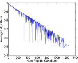
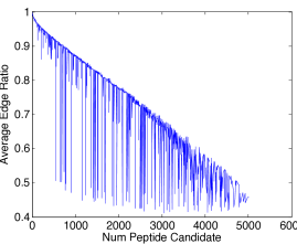
Figure 8: Lattice Compression Ratio: for mass windows of certain number of peptide candidates, calculate the number of edges in the corresponding lattices divided by the number of peaks in the candidates from Yeast(left)/Worm(right) databases.

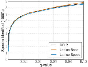
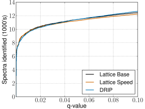
Figure 9: Performance curves: compare two lattice results against the original DRIP, on Yeast (left) and Worm-I (right) with charge 2.

To illustrate the effectiveness of improving inference time using lattices, we test Lattice DRIP with the following beam pruning strategies, and compare the results against DRIP (using the beam pruning settings described in [4]):

• $lattice_{base}$: pruning with $k$-beams which are dynamic across time frames, with wider beams for the early part and narrower beams later on.

• $lattice_{speed}$: pruning aggressively with dynamic $k$-beam (same as $lattice_{base}$) with narrower beams. Moreover, the pbeam pruning algorithm is applied, which prunes the state space while building up the inference structures.

Table 1: Percentage running time of lattice methods compared to original DRIP.

dataset	$lattice_{speed}$	$lattice_{base}$	DRIP
Yeast	7.78%	14.80%	100%
Worm-I	8.59%	16.36%	100%

We note that while the space of beam pruning strategies is large and it is possible that the two above methods are not optimal in terms of absolute computational efficiency achievable using lattices, they give significant speed improvements over the original DRIP. To evaluate the speed-ups possible with lattices, we randomly select 50 spectra from Yeast and Worm-I, respectively, and record inference time. We use the same graphical model inference engine for all three methods. Experiments were carried out on a 3.40GHz CPU with 16G memory. The lowest CPU time out of 3 runs is recorded, and we report the relative CPU time of lattice methods to original DRIP in Table 1. Timing tests show that utilizing lattices, DRIP runs 7-15 times faster. Note that this comes at practically no expense to performance, as show in Figure 9.

8.3 Discriminative training further boosts statistical power

As detailed in Section 6, we use a set of high-confidence, charge 2+ PSMs and their corresponding peptide database to discriminatively train DRIP, utilizing lattices in the denominator model. To illustrate the power afforded by DRIP’s learning capabilities, we also illustrate performance under hand-tuned parameters, where DRIP’s Gaussian means are placed between unit intervals along the m/z access (representative of fixed binning strategies). Figures 10(a), 10(b) show that the discriminatively trained DRIP improves performance, especially for low $q$-values, arguably the most important region of performance. Note that the discriminatively trained model depicted employs the $lattice_{base}$ pruning strategy, and thus we have an increase in accuracy as well an approximately seven-fold speed-up.

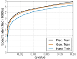
(a) Yeast, charge 2+

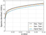
(b) Worm-I, charge 2+

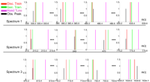
(c) Means used to score observed peaks.

Figure 10: Effects of training DRIP parameters.

In Figure 10(c), we further investigate the influence of training methods on the m/z Gaussian means of DRIP and their performance. Choosing three spectra from Yeast at random, four high intensities are displayed per spectrum, along with the means used to score these peaks. With the observed peaks plotted in black, the resulting discriminatively trained Gaussian means are much closer than all other means, yielding better scoring and more accurate results.

9 Conclusions

In this paper, we show several significant improvements to the DRIP model. We show how to apply word lattices to compress peptide candidate sets in order to dramatically speed up inference in DRIP (7-15 fold speed up). With the ability to compactly represent entire sets of peptides, we extend DRIP’s learning framework to discriminative training, leading to performance gains at low $q$-values. We have also greatly simplified the DRIP model itself and allowed the ability to accurately search varying charge states per dataset.

There are several avenues for future work. With the ability to effienctly sequence through entire set peptides afforded by lattices, we will investigate ways to take thresholds with respect to DRIP scores in order to compute p-values. As evidenced by other scores for which exact p-values are computed (MS-GF+, XCorr p-value), this is expected to greatly increase DRIP’s performance. We have also only scratched the surface of training parameters with the model. Collecting an assortment of training data, we will discriminatively train the model for a host of different charge states, machine types, and organisms in an effort to further increase accuracy over the wide array of tandem mass spectra encountered in practice. We also plan to explore ways to alleviate the labor intensive process of collecting high-confidence training PSMs described in [11], in order to simplify the overall training process, beginning from data collection.

References

- [1] Diament, B., Noble, W.S.: Faster sequest searching for peptide identification from tandem mass spectra. Journal of Proteome Research 10(9), 3871–3879 (2011), pMC3166376
- [2] Eng, J.K., McCormack, A.L., Yates, III, J.R.: An approach to correlate tandem mass spectral data of peptides with amino acid sequences in a protein database. Journal of the American Society for Mass Spectrometry 5, 976–989 (1994)
- [3] Eng, J.K., Jahan, T.A., Hoopmann, M.R.: Comet: An open-source ms/ms sequence database search tool. Proteomics 13(1), 22–24 (2013)
- [4] Halloran, J.T., Bilmes, J.A., Noble, W.S.: Learning peptide-spectrum alignment models for tandem mass spectrometry. In: Uncertainty in Artificial Intelligence (UAI). AUAI, Quebic City, Quebec Canada (July 2014)
- [5] Hopcroft, J.: An n log n algorithm for minimizing states in a finite automaton (1971)
- [6] Howbert, J.J., Noble, W.S.: Computing exact p-values for a cross-correlation shotgun proteomics score function. Molecular & Cellular Proteomics pp. mcp–O113 (2014)
- [7] Ji, G., Bilmes, J., Michels, J., Kirchhoff, K., Manning, C.: Graphical model representations of word lattices ieee/acl 2006 workshop on spoken language technology (slt2006) , palm beach, aruba, dec 2006. IEEE/ACL Workshop on Spoken Language Technology (SLT) (2006)
- [8] Käll, L., Canterbury, J., Weston, J., Noble, W.S., MacCoss, M.J.: A semi-supervised machine learning technique for peptide identification from shotgun proteomics datasets. Nature Methods 4, 923–25 (2007)
- [9] Käll, L., Storey, J.D., MacCoss, M.J., Noble, W.S.: Assigning significance to peptides identified by tandem mass spectrometry using decoy databases. Journal of Proteome Research 7(1), 29–34 (2008)
- [10] Kim, S., Mischerikow, N., Bandeira, N., Navarro, J.D., Wich, L., Mohammed, S., Heck, A.J., Pevzner, P.A.: The generating function of CID, ETD, and CID/ETD pairs of tandem mass spectra: applications to database search. Molecular and Cellular Proteomics 9(12), 2840–2852 (2010)
- [11] Klammer, A.A., Reynolds, S.M., Bilmes, J.A., MacCoss, M.J., Noble, W.S.: Modeling peptide fragmentation with dynamic Bayesian networks for peptide identification. Bioinformatics 24(13), i348–356 (Jul 2008), http://bioinformatics.oxfordjournals.org/cgi/content/abstract/24/13/i348
- [12] McIlwain, S., Tamura, K., Kertesz-Farkas, A., Grant, C.E., Diament, B., Frewen, B., Howbert, J.J., Hoopmann, M.R., Käll, L., Eng, J.K., et al.: Crux: rapid open source protein tandem mass spectrometry analysis. Journal of proteome research (2014)
- [13] Nesvizhskii, A.I.: A survey of computational methods and error rate estimation procedures for peptide and protein identification in shotgun proteomics. Journal of Proteomics 73(11), 2092 – 2123 (2010)
- [14] Watson, B.W.: A taxonomy of finite automata minimization algorithms. Computer Science Note 44 (93)