Mean and variance estimation in high-dimensional heteroscedastic models with non-convex penalties

Abstract

Despite its prevalence in statistical datasets, heteroscedasticity (non-constant sample variances) has been largely ignored in the high-dimensional statistics literature. Recently, studies have shown that the Lasso can accommodate heteroscedastic errors, with minor algorithmic modifications (Belloni et al., 2012; Gautier and Tsybakov, 2013). In this work, we study heteroscedastic regression with a linear mean model and a log-linear variances model with sparse high-dimensional parameters. We propose estimating variances in a post-Lasso fashion, which is followed by weighted-least squares mean estimation. These steps employ non-convex penalties as in Fan and Li (2001), which allows us to prove oracle properties for both post-Lasso variance and mean parameter estimates. We reinforce our theoretical findings with experiments.

Keywords. heteroscedasticity, high dimensional regression, variance estimation, model selection, HIPPO

1 Introduction

Statistical inference in high-dimensions addresses the problem of extracting meaningful information from datasets where the number of variables $p$ can be significantly larger than $n$. In order to adapt linear regression to the high-dimensional regime, the statistical and algorithmic efficiency of penalized least squares methods have been extensively studied. Among the most prominent of such procedures is the Lasso (Tibshirani, 1996), Adaptive Lasso (Huang et al., 2008), and the SCAD penalty (Fan and Li, 2001). The majority of this work has focused on mean estimation in the homoscedastic setting, in which the sample variances are identical. In the classical, low-dimensional, setting the effect of heteroscedasticity and the estimation of variance parameters has been extensively studied (Rutemiller and Bowers, 1968; Carroll et al., 1988) Recent studies have addressed the problem of mean estimation under heteroscedasticity in high-dimensions, where the sample variances may differ (Belloni et al., 2012; Gautier and Tsybakov, 2013). While much of this work has shown that penalized least squared procedures retain their statistical guarantees under mild heteroscedasticity, little work has focused on jointly performing model selection for both mean and variances. In this work, we study a simple procedure for estimating both the mean and variance parameters and examine its ability to correctly identify the sparsity pattern and its asymptotic distribution.

Throughout this work, we assume that we have the usual heteroscedastic Gaussian linear model,

$$y_{i}=\mathbf{x}_{i}^{\prime}\bm{\beta}^{\star}+\sigma(\mathbf{x}_{i},\bm{\theta}^{\star})\epsilon_{i},\quad i=1,\ldots,n,$$ (1)

where $\mathbf{x}_{i}\in\mathbb{R}^{p}$ are the observed covariates, $\bm{\theta}^{\star},\bm{\beta}^{\star}\in\mathbb{R}^{p}$ are unknown parameter, $\{\epsilon_{i}\}_{i=1}^{n}$ are independent, normally distributed with mean $0$ and variance $1$ and the function $\sigma$ is of log-linear form,

$$2\log\sigma(\mathbf{x}_{i},\bm{\theta})=\mathbf{x}_{i}^{\prime}\bm{\theta}.$$ (2)

Modeling the log variance as a linear combination of the explanatory variables, as in (2) is a common choice as it guarantees positivity and is also capable of capturing variance that may vary over several orders of magnitudes (Carroll and Ruppert, 1988; Harvey, 1976a). In this paper, we study penalized estimation of the high-dimensional heteroscedastic linear regression model, (1), where $p\gg n$.

We study a natural procedure for estimating the mean and variance parameters, called heteroscedastic iterative penalized pseudolikelihood optimizer (HIPPO) first proposed in (Kolar and Sharpnack, 2012). This method assumes that a mean estimation procedure such as the lasso is first performed, and then using this mean estimate, one performs model selection for the variance parameter. Finally, an updated mean parameter is constructed with a regularized weighted least squares procedure. Thus HIPPO not only outputs a heteroscedasticity aware mean parameter estimate, but also provides variance parameter estimates. With these parameters the practitioner has an estimate for the predictive distribution given a new sample (by plugging in the estimates $\widehat{\bm{\beta}},\widehat{\bm{\theta}}$). Aside from providing superior mean estimates, a primary reason to model variances is that it provides us with estimated predictive distributions. Furthermore, determining which covariates drive the variance may be of scientific interest. In economics and finance, volatility of macroeconomic variables and financial instruments is of significant interest. (In economic time series heteroscedasticity is modeled in an autoregressive conditional heteroscedastic (ARCH) model (Engle, 1982).) When rating insurance policies, it is common practice to fit both mean and dispersion parameters in double generalized linear models (Peters et al., 2009), which is a class that the heteroscedastic Gaussian model falls into. In environmental modeling, climate variability has been recognized as one of the hallmarks of global climate change and has been added to the discussion surrounding the impact of human activity on the environment (Karl et al., 1995). More generally, extreme event probabilities are driven primarily by the variance of the predictive distribution for the model, (1), so for any application where extreme events are of interest, estimating variances is essential.

Of separate interest is providing confidence regions for mean parameters in high-dimensions under heteroscedasticity. The confidence of an estimate of $\beta_{j}^{\star}$ ($j\in\{1,\ldots,p\}$) will be driven by the variances of the samples $\{\sigma(\mathbf{x}_{i},\bm{\theta}^{\star})\}_{i=1}^{n}$ in relation to the $j$th covariate $\{\mathbf{x}_{i,j}\}_{i=1}^{n}$. We will see that, given our assumptions, our mean parameter estimates will obtain a specific asymptotic distribution. This distribution can be inverted to obtain simple confidence region for $\bm{\beta}^{\star}$ that is asymptotically valid given our conditions.

The main contributions of this paper are as follows. First, we review the HIPPO (Heteroscedastic Iterative Penalized Pseudolikelihood Optimizer) for estimation of both the mean and variance parameters, and propose some changes to the method. Second, we establish theoretical guarantees in the form of oracle properties (in the sense of Fan and Lv (2009)) for the estimated mean and variance parameters. These are significantly superior to the theoretical guarantees in (Kolar and Sharpnack, 2012) because they require much more mild assumptions. We examine some numerical properties of the proposed procedure on a simulation study to complement our theoretical findings.

1.1 Notation

Throughout this work matrices and vectors are bolded while scalars are not. We will let $\mathbf{X}=(\mathbf{x}_{1},\ldots,\mathbf{x}_{n})^{\prime}=(\mathbf{X}_{1},\ldots,\mathbf{X}_{p})$ denote the $n\times p$ matrix of predictors, $\mathbf{y},\bm{\epsilon}$ are the $n$-vector of responses, and noise respectively. We will use $O()$ and $o()$ notation to indicate boundedness and convergence of sequences and their probabilistic counterparts $O_{\mathbb{P}}(),o_{\mathbb{P}}()$. Throughout the paper we use $[n]$ to denote the set $\{1,\ldots,n\}$. For any index set $S\subseteq[p]$, we denote $\bm{\beta}_{S}$ to be the subvector containing the components of the vector $\bm{\beta}$ indexed by the set $S$, and $\mathbf{X}_{S}$ denotes the submatrix containing the columns of $\mathbf{X}$ indexed by $S$. For a vector $\mathbf{a}\in\mathbb{R}^{n}$, we denote ${\rm supp}(\mathbf{a})=\{j\ :\ a_{j}\neq 0\}$ the support set, $||\mathbf{a}||_{q}$, $q\in(0,\infty)$, the $\ell_{q}$-norm defined as $||\mathbf{a}||_{q}=(\sum_{i\in[n]}a_{i}^{q})^{1/q}$ with the usual extensions for $q\in\{0,\infty\}$, that is, $||\mathbf{a}||_{0}=|{\rm supp}(\mathbf{a})|$ and $||\mathbf{a}||_{\infty}=\max_{i\in[n]}|a_{i}|$. For notational simplicity, we denote $||\cdot||=||\cdot||_{2}$ the $\ell_{2}$ norm. For a matrix $\mathbf{A}\in\mathbb{R}^{n\times p}$ we denote $|\!|\!|\mathbf{A}|\!|\!|_{{2}}$ the operator norm, $||\mathbf{A}||_{F}$ the Frobenius norm, and $\Lambda_{\min}(\mathbf{A})$ and $\Lambda_{\max}(\mathbf{A})$ denote the smallest and largest eigenvalue respectively.

1.2 Related work

Heteroscedasticity in low-dimensions. Variance parameter estimation in low-dimensions began with the study of linear forms for the variance, and extended to higher degree polynomial forms (Rutemiller and Bowers, 1968; Geary, 1966; Lancaster, 1968). The estimation of parameters of the variance when it takes on a log-linear form in low-dimensions was comprehensively studied in Harvey (1976b). The author concluded that maximum likelihood, estimated with the iterative ‘method of scoring’, had a significantly better asymptotic variance than previous methods proposed. Carroll et al. (1988) studied a more general iterative procedure for variance estimation, specifically they proved limiting distributions for the mean parameter estimates after a fixed number of iterations.

Another classical approach to estimating variances in the heteroscedastic Gaussian linear model is to use a restricted likelihood for the estimating equation (Patterson and Thompson, 1971). The basic idea is that one can separate the data $\mathbf{y}$ into two orthogonal components, one of which is ancillary to $\bm{\beta}^{\star}$. This way the variance parameter $\bm{\theta}^{\star}$ can be estimated from that component by maximizing its marginal likelihood, forming the residual (or restricted) maximum likelihood (REML). Unfortunately, this method is only valid when $p<n$, so is not suitable for our purposes.

More recently non-parametric procedures were constructed to estimate variances under heteroscedasticity. Rigby and Stasinopoulos (1996) proposed a general procedure by which a generalized additive model could be estimated for both the mean and variance (in low dimensions). Fan and Yao (1998) studied local linear estimates for the mean and similarly estimating the variance from the resulting residuals. Other estimators were constructed from similar procedures under logarithmic transformations of the residuals (Yu and Jones, 2004; Chen et al., 2009). None of these methods are appropriate in high-dimensions because they do not perform model-selection under a sparsity assumption.

Of separate interest is the effect that heteroscedasticity has on standard regression procedures that assume homoscedasticity. While it is the case that ordinary least squares (OLS) is consistent and enjoys a central limit theorem despite heteroscedasticity (under mild conditions), the classical estimate of standard errors is no longer consistent (Eicker, 1967). In a landmark paper, White (1980) showed that with minimal assumptions an estimate of standard errors could be formed by estimating directly the asymptotic variance of OLS coefficients. Rao (1970) developed an estimator for linear functionals of the variances which is asymptotically equivalent to that of White (1980). This work falls more generally under the moniker generalized estimating equations (GEE), in which one presupposes that the likelihood is misspecified and one attempts to quantify the effect of misspecification on the maximum likelihood estimates (Ziegler, 2011; Royall, 1986). (In this way, the supposed likelihood is called a pseudo-likelihood, which is a name that we will be using throughout this work.)

High dimensional regression. The penalization of the empirical loss by the $\ell_{1}$ norm has become a popular tool for obtaining sparse models and a vast amount of literature exists on theoretical properties of estimation procedures (see,e.g., Zhao and Yu, 2006; Wainwright, 2009; Zhang, 2009; Zhang and Huang, 2008, and references therein) and on efficient algorithms that numerically find estimates (see Bach et al., 2011, for an extensive literature review). Due to limitations of the $\ell_{1}$ norm penalization, high-dimensional inference methods based on the class of concave penalties have been proposed that have better theoretical and numerical properties (see, e.g., Fan and Li, 2001; Fan and Lv, 2009; Lv and Fan, 2009; Zhang and Zhang, 2011).

The HIPPO procedure employs a non-convex penalty function to impose sparsity in the estimates. Nonconvex penalties are commonly used to reduce bias in estimation. A number of authors have proposed non-convex penalties, including smoothly clipped absolute deviations (SCAD) (Fan and Li, 2001), minimax concave (MC) penalty (Zhang, 2010a), and capped $\ell_{1}$ (Zhang, 2010b, 2013). See Fan and Lv (2010) for a recent survey. The oracle estimator is a local solution to the optimization problem (Kim et al., 2008; Fan and Lv, 2011). However, finding this particular solution is problematic in practice. A number of recent papers have studied properties of local solutions obtained by particular numerical procedures (Zhang (2010b), Zhang (2013), Wang et al. (2013a), Loh and Wainwright (2013), Fan et al. (2012), Wang et al. (2013b)). Under suitable conditions on the design matrix and the signal size, Fan et al. (2012) and Loh and Wainwright (2013) establish that two step procedures obtain the oracle solution. However, these conditions are quite restrictive. Properties of global solution to non-convex problem were studied in Kim and Kwon (2012); Zhang and Zhang (2012).

There have been recent advances on providing mean estimates in high dimensions that can handle heteroscedastic errors. Belloni et al. (2012) provide an algorithm that adapts the $\ell_{1}$ penalty to compensate for the effect of different sample variances. Similarly, Gautier and Tsybakov (2013), introduce a family of $\ell_{1}$ minimization methods called the self-tuned Dantzig estimator which has been shown to handle heteroscedastic errors. The HIPPO algorithm will use the method of Belloni et al. (2012) to provide an initial estimate for $\bm{\beta}^{\star}$. There has also been some recent work addressing the estimation of variance parameters in high dimensions. Notably, Daye et al. (2012) proposes the HHR procedure, that iteratively performs $\ell_{1}$ penalized likelihood minimizations, but do not provide statistical guarantees. Cai and Wang (2008) developed a wavelet thresholding procedure that is adaptive to the smoothness of the mean and variance functions, but the results are difficult to extend to non-orthogonal design matrices. Dalalyan et al. (2013) proposes a second-order convex program with group penalties to estimate the mean and variance parameters jointly. They avoid the likelihoods non-convexity by performing a transformation that makes the likelihood jointly convex, but the choice of transformation (however convenient from an algorithmic standpoint) does not coincide with the log-linear variance model that we consider here.

2 Methodology

The primary difficulty with jointly estimating the mean and variance parameters, even in the low dimensional setting (where $p$ is fixed and $n\rightarrow\infty$) is that the likelihood for the model (1) is not jointly convex in $\bm{\beta}$ and $\bm{\theta}$. Indeed, the negative log-likelihood for the mean and variance parameters is

$$\ell(\bm{\beta},\bm{\theta};\mathbf{y},\mathbf{X})=\sum_{i=1}^{n}(y_{i}-\mathbf{x}_{i}\bm{\beta})^{2}\exp(-\mathbf{x}_{i}^{\prime}\bm{\theta})+\mathbf{x}_{i}^{\prime}\bm{\theta},$$ (3)

up to additive constants. Because the likelihood with $\bm{\theta}$ fixed is convex in $\bm{\beta}$ and vice versa, a coordinate descent method with a regularized likelihood is a natural approach to joint estimation. In (Kolar and Sharpnack, 2012), a simplified method called HIPPO was proposed, where only the first few iterations of the coordinate descent procedure are performed.

The justification for stopping the coordinate descent procedure early is derived from pseudolikelihood theory. Suppose that we have an initial mean estimate $\widehat{\bm{\beta}}$, then if we consider minimizing $\ell(\widehat{\bm{\beta}},\bm{\theta};\mathbf{y},\mathbf{X})$ with $\widehat{\bm{\beta}}$ fixed, resulting in $\widehat{\bm{\theta}}$, then if $\widehat{\bm{\beta}}$ is close to $\bm{\beta}^{\star}$ then $\widehat{\bm{\theta}}$ will be close to the minimizer of $\ell(\bm{\beta}^{\star},\bm{\theta};\mathbf{y},\mathbf{X})$. We then think of $\ell(\bm{\beta}^{\star},\bm{\theta};\mathbf{y},\mathbf{X})$ as the true likelihood, and $\ell(\widehat{\bm{\beta}},\bm{\theta};\mathbf{y},\mathbf{X})$ as the pseudo-likelihood. HIPPO works because the initial lasso procedure produces an estimate for $\widehat{\bm{\beta}}$ which is good enough in the sense that the pseudo-likelihood is a good approximation of the true likelihood for $\bm{\theta}^{\star}$. In this paper, we propose some modifications to that algorithm and show that under mild conditions this performs as well as the oracle procedures (where the fixed parameter and the support set of the free parameter is known). Throughout this work we will consider a penalty function, $\rho_{\lambda}:\mathbb{R}_{+}\to\mathbb{R}_{+}$, which has the effect of enforcing the sparsity in the resulting estimates.

HIPPO is comprised of three steps (which we will refer to as stages):

1. HIPPO solves a LASSO program (Algorithm A1 in Belloni et al. (2012)) for estimating $\bm{\beta}^{\star}$ resulting in $\widehat{\bm{\beta}}$.

2. HIPPO forms the penalized pseudo-likelihood estimate for $\bm{\theta}^{\star}$ by solving

   $$\widehat{\bm{\theta}}=\arg\min_{\bm{\theta}\in\mathbb{R}^{p}}\sum_{i=1}^{n}\mathbf{x}_{i}^{\prime}\bm{\theta}+\sum_{i=1}^{n}\widehat{\eta}_{i}^{2}\exp(-\mathbf{x}_{i}^{\prime}\bm{\theta})+4n\sum_{j=1}^{p}\rho_{\lambda_{j}^{T}}(|\theta_{j}|)$$ (4)

   where $\widehat{\bm{\eta}}=\mathbf{y}-\mathbf{X}\widehat{\bm{\beta}}$ is the vector of residuals. Furthermore, $\lambda_{j}^{T}=\lambda_{T}\|\mathbf{X}_{j}\|/n$ for $j\in[p]$, where $\lambda_{T}$ is an appropriately chosen tuning parameter.

3. Finally, HIPPO computes the reweighted estimator of the mean by solving

   $$\widehat{\bm{\beta}}_{w}=\arg\min_{\bm{\beta}\in\mathbb{R}^{p}}\sum_{i=1}^{n}\frac{(y_{i}-\mathbf{x}_{i}^{\prime}\bm{\beta})^{2}}{\widehat{\sigma}^{2}_{i}}+2n\sum_{j=1}^{p}\rho_{\lambda_{j}^{S}}(|\beta_{j}|)$$ (5)

   where $\widehat{\sigma}_{i}=\exp(\mathbf{x}_{i}^{\prime}\widehat{\bm{\theta}}/2)$ are the weights. Likewise, $\lambda^{S}_{j}=\lambda_{S}n^{-1}\sqrt{\sum_{i=1}^{n}x_{i,j}^{2}/\widehat{\sigma}_{i}^{2}}$ for an appropriately chosen tuning parameter $\lambda_{S}$.

The details of HIPPO differ here from (Kolar and Sharpnack, 2012) in the choice of penalty parameters $\bm{\lambda}^{T},\bm{\lambda}^{S}$ and that stage 1 here uses the LASSO procedure with heteroscedasticity adjusted penalties of Belloni et al. (2012). These modifications enable us to demonstrate that HIPPO enjoys significantly stronger theoretical guarantees than those established in Kolar and Sharpnack (2012).

As was mentioned, the intuition behind HIPPO is that with the estimate, $\widehat{\bm{\beta}}$, from stage 1 we can form a penalized pseudo-likelihood for $\bm{\theta}$ given by (4). We call this a pseudo-likelihood, because it can be thought of as an approximation to the likelihood function for $\bm{\theta}^{\star}$ with $\bm{\beta}^{\star}$ known. In classical statistics literature, it is common in misspecified models to consider maximum likelihood methods as minimizers of an objective function that differs from the true likelihood. Central limit theorems have been derived for such maximum pseudo-likelihood estimators using generalized estimating equations (Ziegler, 2011). Similarly, in stage 3, the act of reweighting in effect makes the penalized pseudo-likelihood in (5) much closer to the true penalized likelihood with known $\bm{\theta}^{\star}$.

HIPPO is closely related to the iterative HHR algorithm of Daye et al. (2012). HIPPO differs for HHR by the choice of penalty functions and by the fact that we advocate only running the three stages of HIPPO as opposed to continuing to iterate stages 2 and 3 with the updated $\bm{\beta}$ and $\bm{\theta}$ parameters. This recommendation is justified by theoretical and experimental results.

2.1 Properties of the penalty

The penalty function, $\rho_{\lambda}$, is chosen so that the resulting estimates satisfy three properties: unbiasedness, sparsity and continuity. The sparsity condition means that our estimator has the same support as the true parameter with probability approaching $1$ (a property commonly known as sparsistency). Unlike the lasso, our penalties are chosen so that when the signal size is strong enough the penalty does not incur a bias on the reconstructed signal. To provide us with a theoretical comparison, we can think about the maximum likelihood estimators that we could construct with the knowledge of the true sparsity sets, $S={\rm supp}(\bm{\beta}^{\star})$ and $T={\rm supp}(\bm{\theta}^{\star})$. We call these estimators the oracle estimators. It is our goal to provide minimal conditions under which HIPPO attains the same asymptotic distribution as the oracle estimators, and we call this the oracle property. The asymptotic unbiasedness assumption is critical if we hope that HIPPO will achieve the oracle property.

Concave penalty functions are known to admit solutions that are asymptotically unbiased. Examples are the smoothly clipped absolute deviation (SCAD) penalty (Fan and Li, 2001), the minimax concave (MC) penalty (Zhang, 2010a) and a class of folded concave penalties (Lv and Fan, 2009). The SCAD penalty can be defined by its derivative,

$$\rho_{\lambda}^{\prime}(\beta)=\lambda\left[I\{|\beta|\leq\lambda\}+\frac{(a\lambda-|\beta|)_{+}}{(a-1)\lambda}I\{|\beta|>\lambda\}\right],$$ (6)

where $a>2$ is a fixed parameter and $\rho_{\lambda}(0)=0$. The intuition behind the specific form for SCAD is that for a neighborhood around $0$ it acts like the $\ell_{1}$ penalty, shrinking small components toward $0$. While further from $0$ the effect of the penalty diminishes until it becomes constant for large enough values of $\beta$. Hence, the shrinkage effect is reduced for larger components, resulting in zero bias in these coordinates.

More generally, the penalty function is assumed to satisfy the following properties

1. $\rho_{\lambda}(0)=0.$

2. The function $\rho_{\lambda}$ satisfies $\rho_{\lambda}(\beta_{0}+\beta_{1})\leq\rho_{\lambda}(\beta_{0})+\rho_{\lambda}(\beta_{1})$ for all $\beta_{0},\beta_{1}\geq 0$.

3. The derivative $\rho^{\prime}_{\lambda}(\beta)$ is continuous on $\beta\in(0,\infty)$ and normalized so that $\lim_{\beta\rightarrow 0+}\rho^{\prime}_{\lambda}(\beta)=\lambda$.

4. There exists a constant $b>0$ such that

   $$\rho_{\lambda}^{\prime}(\beta) \leq\lambda,\forall 0<\beta<b\lambda$$

   $$\rho_{\lambda}^{\prime}(\beta) =0,\forall\beta\geq b\lambda.$$

All of the aforementioned concave penalties satisfy the above conditions. For example, the MC penalty (Zhang, 2010a) is likewise defined by its derivative,

$$\rho_{\lambda}^{\prime}(\beta)=\frac{(a\lambda-\beta)_{+}}{a},$$ (7)

where $a>0$ is a fixed parameter and (P1)-(P4) can be verified.

2.2 Tuning Parameter Selection and Optimization Procedure

The optimization programs of (4) and (5) require the selection of the tuning parameters $\lambda_{S}$ and $\lambda_{T}$, which balance the propensity to overfit to the data with a complex model and the underfitting when the penalty is too harsh. A common approach, and the one that we take, is to form a grid of candidate values for the tuning parameters $\lambda_{S}$ and $\lambda_{T}$ and chose those that minimize the AIC or BIC criterion

$${\rm AIC}(\lambda_{S},\lambda_{T})=\ell(\widehat{\bm{\beta}},\widehat{\bm{\theta}};\mathbf{y},\mathbf{X})+2\widehat{df},$$ (8)

$${\rm BIC}(\lambda_{S},\lambda_{T})=\ell(\widehat{\bm{\beta}},\widehat{\bm{\theta}};\mathbf{y},\mathbf{X})+\widehat{df}\log n$$ (9)

where

$$\widehat{df}=|{\rm supp}(\widehat{\bm{\beta}})|+|{\rm supp}(\widehat{\bm{\theta}})|$$

is the estimated degrees of freedom. In Section 4, we evaluate the performance of the AIC and the BIC for HIPPO in experiments.

While our theoretical results hold for any penalty function, $\rho_{\lambda}$, with properties (P1)-(P4), in all of our experiments we will use the SCAD penalty defined by (6). We now describe our choice of numerical procedures used to solve the optimization problems in (4) and (5). These methods are based on the local linear approximation for the SCAD penalty developed in Zou and Li (2008),

$$\rho_{\lambda}(|\beta_{j}|)\approx\rho_{\lambda}(|\beta_{j}^{(k)}|)+\rho_{\lambda}^{\prime}(|\beta_{j}^{(k)}|) (|\beta_{j}|-|\beta_{j}^{(k)}|),\quad\text{for }\beta_{j}\approx\beta_{j}^{(k)}.$$

With this approximation, we can substitute the SCAD penalty $\sum_{j\in[p]}\rho_{\lambda}(|\beta_{j}|)$ in (4) and (5) with

$$\sum_{j=1}^{p}\rho_{\lambda}^{\prime}(|\widehat{\beta}_{j}^{(k)}|)|\beta_{j}|,$$ (10)

and iteratively solve each objective until convergence of $\{\widehat{\bm{\beta}}^{(k)}\}_{k}$. We set the initial estimates $\widehat{\bm{\beta}}^{(0)}$ and $\widehat{\bm{\theta}}^{(0)}$ to be the solutions of the $\ell_{1}$-norm penalized problems. The convergence of these iterative approximations follows from the convergence of the MM (minorize-maximize) algorithms (Zou and Li, 2008). Recent work has demonstrated that iterative algorithms utilizing local linear expansions of concave penalties have oracle properties (for mean estimation) that hold without the restricted eigenvalue condition (Wang et al., 2013b; Fan et al., 2014; Wang et al., 2013a).

With the approximation of the SCAD penalty given in (10), we can solve (5) using standard lasso solvers, for example, we use the proximal method of Beck and Teboulle (2009). The objective in (4) is minimized using a coordinate descent algorithm, which is detailed in Daye et al. (2012).

3 Theoretical Guarantees

Throughout this section, we will be using the following notation to denote sub-polynomial functions, and polynomial-type decay. These definitions will be used in the conditions statement and are used throughout the Appendix.

Definition 1.

We say that a function $f(n)$ is sub-polynomial if

$$\forall\gamma>0,\quad f(n)=o(n^{\gamma})$$

and we denote this by $f(n)=\tilde{O}(1)$. We also say that $f(n)$ has polynomial decay if

$$\exists\gamma>0,\quad f(n)=O(n^{-\gamma})$$

and we denote this with $f(n)=\tilde{o}(1)$.

Because the penalties that we are using are necessarily non-convex, we will not in general have a unique minimum for the program (4). As a result, our guarantees will state that there exists a local minimizer that has guarantees similar to what we could achieve had we known the set $T={\rm supp}(\bm{\theta}^{\star})$ and the parameter $\bm{\beta}^{\star}$. In this sense we say that this local minimizer enjoys oracle properties. There is a strong precedent for this style of results in the non-convex penalty literature of Fan and Li (2001); Fan and Lv (2011). Theoretical results of this type suffer from the possibility that the optimization algorithm used may in fact not select this local minimizer, but will instead converge to a local minimum with poor performance. These fears will be assuaged by simulation studies.

We will begin our analysis of the second stage program (4), by considering the variance estimator when $\bm{\beta}^{\star}$ is known and we set $\widehat{\bm{\beta}}=\bm{\beta}^{\star}$. This will serve both as a benchmark and a lemma for the theoretical guarantees of the pseudo-likelihood optimizer in stage 2 (with $\bm{\beta}^{\star}$ unknown).

3.1 Variance estimation with $\bm{\beta}^{\star}$ known.

In the unlikely event that the mean parameter $\bm{\beta}^{\star}$ is known, the program (4) may now be considered a true likelihood. In this setting, we will derive the oracle properties by showing that the oracle maximum likelihood estimate (OMLE), the MLE when the sparsity set $T={\rm supp}(\bm{\theta}^{\star})$ is known, is a local minimizer of (4). As is standard in maximum likelihood theory, we achieve this by examining conditions under which this likelihood is well approximated by its elliptical contours. The requisite assumptions are listed below.

1. Define $T={\rm supp}(\bm{\theta}^{\star})$.

   $$|\!|\!|\mathbf{X}_{T}|\!|\!|_{{2,\infty}}=O\left(\sqrt{t\log p}\right)$$

   $$\sum_{i}\|\mathbf{x}_{i,T}\|^{2}=O\left(nt\right)$$

   $$\sum_{i}\|\mathbf{x}_{i,T}\|^{3}=O\left(nt^{3/2}\right)$$

2. Define the empirical covariance Tensors for $k=2,3,4,6$,

   $$\widehat{\Sigma}=\frac{1}{n}\sum_{i=1}^{n}\mathbf{x}_{i}\mathbf{x}_{i}^{\prime},\quad\widehat{\Sigma}^{(k)}=\frac{1}{n}\sum_{i=1}^{n}\mathbf{x}_{i}^{\otimes k}$$

   Let the following be the largest eigenvalues for the restricted Tensors,

   $$\Lambda_{\max}\left(\widehat{\Sigma}_{TT}\right)=\sup_{\|\mathbf{z}\|=1}\frac{1}{n}\sum_{i=1}^{n}(\mathbf{x}_{i,T}^{\prime}\mathbf{z})^{2},\quad\Lambda_{\max}\left(\widehat{\Sigma}^{(k)}_{T}\right)=\sup_{\|\mathbf{z}\|=1}\frac{1}{n}\sum_{i=1}^{n}(\mathbf{x}_{i,T}^{\prime}\mathbf{z})^{k}$$

   then we assume that these are not divergent,

   $$\Lambda_{\max}\left(\widehat{\Sigma}_{TT}\right)=O(1),\quad\Lambda_{\max}\left(\widehat{\Sigma}_{T}^{(k)}\right)=O(1).$$

   And we further assume that the covariance is not singular (asymptotically).

   $$\Lambda_{\min}\left(\widehat{\Sigma}_{TT}\right)=\inf_{\|\mathbf{z}\|=1}\frac{1}{n}\sum_{i=1}^{n}(\mathbf{x}_{i,T}^{\prime}\mathbf{z})^{2}>c_{2}$$

   for some constant $c_{2}$ and $n$ large enough.

We are finally prepared to state the oracle properties of our variance estimator with known mean.

Theorem 2.

Consider the non-convex program in stage 2, (4), with $\widehat{\bm{\beta}}=\bm{\beta}^{\star}$ and assume (A1),(A2). Assume that $t=|T|$ is subpolynomial in $\sqrt{n}$, $t=\tilde{o}(\sqrt{n})$ and suppose that

$$\max_{j\in[p]}\left\|\mathbf{X}_{T}\frac{\mathbf{X}_{j}}{\|\mathbf{X}_{j}\|}\right\|=\tilde{O}\left(n^{-1/4}\right),\quad\max_{i\in[n],j\in[p]}\left|\frac{x_{i,j}}{\|\mathbf{X}_{j}\|}\right|=O((\log p)^{-1/2}),$$ (11)

that $\log p=\tilde{O}(1)$,

$$\overline{\sigma}=\max_{i\in[n]}\sigma_{i}=\tilde{O}(1),\textrm{ and }\underline{\sigma}=\min_{i\in[n]}\sigma_{i}=\tilde{\Omega}(1).$$

We require that the minimal signal size is

$$\min_{j\in T}|\theta^{\star}_{j}|=\omega\left(\frac{\sqrt{\log p}}{\sqrt{n}}\right).$$

Then for any sequence, $\lambda_{T}$, such that

$$\lambda_{T}=o\left(\min_{j\in T}|\theta^{\star}_{j}|\right),\quad\frac{\sqrt{\log p}}{\sqrt{n}}=o(\lambda_{T})$$

there is a local minimizer $\widehat{\bm{\theta}}$ such that $\widehat{\bm{\theta}}_{T^{C}}={\bf 0}$ and it enjoys the following oracle properties,

$$\textrm{If }\mathbf{a}\in\mathbb{R}^{p},\textrm{ such that }v=\lim_{n\rightarrow\infty}\mathbf{a}^{\prime}\widehat{\Sigma}_{TT}^{-1}\mathbf{a}\in\mathbb{R},\quad\textrm{then }\sqrt{n}\mathbf{a}^{\prime}(\widehat{\bm{\theta}}-\bm{\theta}^{\star})\overset{\mathcal{D}}{\rightarrow}\mathcal{N}(0,v).$$ (12)

$$\max_{j\in[n]}n|\mathbf{x}_{j}^{\prime}(\widehat{\bm{\theta}}-\bm{\theta}^{\star})|=O_{\mathbb{P}}\left(\max_{j\in[n]}\left[\sqrt{n\mathbf{x}_{j,T}^{\prime}\widehat{\Sigma}_{TT}^{-1}\mathbf{x}_{j,T}\log p}+\max_{i\in[n]}\mathbf{x}_{j,T}\widehat{\Sigma}_{TT}^{-1}\mathbf{x}_{i,T}\log p\right]\right).$$ (13)

$$||\widehat{\bm{\theta}}-\bm{\theta}^{\star}||{}=O_{\mathbb{P}}\left(\sqrt{\frac{t}{n}}\right).$$ (14)

Remark 3.

(12) is the distribution achieved by the OMLE because $\mathbf{a}^{\prime}\widehat{\Sigma}^{-1}_{TT}\mathbf{a}$ is the oracle Fisher information for the parameter $\mathbf{a}^{\prime}\bm{\theta}^{\star}$. The simultaneous estimation guarantee of $\mathbf{x}_{j}^{\prime}\bm{\theta}^{\star}$ (and hence of $\sigma(\mathbf{x}_{j},\bm{\theta}^{\star})$) in (13) is the result of the Bernstein-type inequality for Chi-squared random variables. (14) demonstrates the rate at which we expect the variance estimate to converge in $\ell_{2}$ norm.

Let us begin with a discussion of the conditions in Theorem 2. (A1), (A2), and the assumption $t=\tilde{o}(\sqrt{n})$ are conditions required for the OMLE to attain convergence rates akin to those obtained by the central limit theorem in fixed intrinsic dimensions (fixed $T$), hence they would be necessary even in low dimensions. A note should be made that we could precisely characterize the order of the logarithmic terms in the convergence, $t=\tilde{o}(\sqrt{n})$, and other similar statements, but we choose not to for ease of presentation. The condition $\log p=\tilde{o}(1)$ allows for $p=n^{k}$ and $p=n^{\log^{k}n}$ for any $k\geq 1$, hence it can accommodate significantly high dimensions. The condition of (11) is an artifact of the fact that we are generally dealing with $\chi^{2}$ random variables in the variance estimation setting, and it seems to be necessary. The assumption that $\overline{\sigma},\underline{\sigma}^{-1}=\tilde{O}(1)$ is satisfied by the subGaussian design if $\|\bm{\theta}^{\star}\|=O(1)$, and due to the exponential form for the variance, (2), in most settings the variance is diverging either subpolynomially or exponentially.

We will refer to (12), (13), (14) collectively as the oracle properties of $\widehat{\bm{\theta}}$. These results state that under some regularity conditions, there is a local minimizer of (4), that achieves the low-dimensional rates of convergence. The minimal signal size that is required has a similar behavior to the rates required by the Lasso for mean estimation under regularity conditions Wainwright (2009). While this result is interesting on its own, Theorem 2 will provide a theoretical benchmark for the unknown mean case.

The difficulty of extending these to the case in which the true mean parameter, $\bm{\beta}^{\star}$, is unknown and we only have an estimate is that it is possible that $\widehat{\bm{\beta}}$ is a function of the variances $\sigma(\mathbf{x}_{i},\bm{\theta}^{\star})$. Because we construct $\widehat{\bm{\theta}}$ by fitting estimated residuals (constructed by removing the estimated mean from the observations $\widehat{\eta}_{i}=y_{i}-\mathbf{x}_{i}^{\prime}\widehat{\bm{\beta}}$) according to (4), this correspondence between mean and variance can significantly alter the pseudo-likelihood and its local minima. In the following section we address these concerns, and show that under mild conditions about the performance of stage 1, there is a local minimizer $\widehat{\bm{\theta}}$ constructed with the estimate $\widehat{\bm{\beta}}$ that attains the same oracle properties as if $\bm{\beta}^{\star}$ was known.

3.2 Variance estimation with $\bm{\beta}^{\star}$ unknown.

We have discussed what is possible when the sample means, $\mathbb{E}y_{i}=\mathbf{x}_{i}^{\prime}\bm{\beta}^{\star}$, are known. Under mild conditions, there is a variance estimate that satisfies the oracle properties, (12), (13), (14), that is also a local minimizer of (4) with $\widehat{\bm{\beta}}=\bm{\beta}^{\star}$. Of course, in practice, we would have to estimate the mean parameter $\bm{\beta}^{\star}$ without knowledge of the unknown variance parameters $\bm{\theta}^{\star}$. We now show that under reasonable assumptions about the mean estimate $\widehat{\bm{\beta}}$, and an assumption that the largest sample variance is subpolynomial, we can obtain the oracle properties for a local minimizer of (4) with no additional assumptions on the design.

Theorem 4.

Consider the non-convex program in stage 2, (4), with $\widehat{\bm{\beta}}$ satisfying

$$\|\widehat{\bm{\beta}}\|_{0}\leq\tilde{o}_{\mathbb{P}}(\sqrt{n}),\quad\|\mathbf{X}(\bm{\beta}^{\star}-\widehat{\bm{\beta}})\|^{2}=\tilde{o}_{\mathbb{P}}(\sqrt{n})$$ (15)

and assume the conditions of Theorem 2 ((A1),(A2), (11), $t=\tilde{o}(\sqrt{n})$, and $\overline{\sigma},\underline{\sigma}^{-1},\log p=\tilde{O}(1)$). Similarly, assume that

$$\min_{j\in T}|\theta^{\star}_{j}|=\omega\left(\frac{\sqrt{\log p}}{\sqrt{n}}\right).$$

Then for any sequence, $\lambda_{T}$, such that

$$\lambda_{T}=o\left(\min_{j\in T}|\theta^{\star}_{j}|\right),\quad\frac{\sqrt{\log p}}{\sqrt{n}}=o(\lambda_{T})$$

there is a local minimizer $\widehat{\bm{\theta}}$ such that $\widehat{\bm{\theta}}_{T^{C}}={\bf 0}$ and it enjoys the oracle properties (12), (13), (14).

Notice that the conditions placed on $\widehat{\bm{\beta}}$, (15), are only that the solution is sparse and has a reasonable prediction error. This mild assumption about the performance of stage 1 allows for there to be a substantial correspondence between the variance and mean parameters ($\bm{\theta}^{\star}$ and $\bm{\beta}^{\star}$). While it may be guessed that the sharing of relevant covariants ($T\cap S\neq\emptyset$ where $S={\rm supp}(\bm{\beta}^{\star})$), not to mention covariate correlations, would be problematic for the pseudo-likelihood minimizer to recover the support of $\bm{\theta}^{\star}$, no such effect is observed. Only the effect of heteroscedasticity on the ability for $\widehat{\bm{\beta}}$ to satisfy (15) are these concerns manifested. These results are obtained by considering the fact that we are minimizing a pseudolikelihood for $\bm{\theta}$ by plugging in the estimate $\widehat{\bm{\beta}}$ and showing that the pseudolikelihood is close enough to the likelihood.

In order to ensure that the stage 1 solution satisfies (15), we must impose the restricted eigenvalue condition. This is a common assumption in the Lasso literature Bickel et al. (2009), and is satisfied by subGaussian design Rudelson and Zhou (2011). We also require that the optimal penalty loadings (to be defined below) in stage 1 are not too large.

1. Consider the restricted set

   $$\Delta_{C,T}=\{\delta\in\mathbb{R}^{p}:\|\bm{\delta}_{T^{C}}\|_{1}\leq C\|\bm{\delta}_{T}\|_{1},\bm{\delta}\neq{\bf 0}\}$$

   then the restricted eigenvalue of $\widehat{\Sigma}$ is

   $$\kappa^{2}_{C}(\widehat{\Sigma})=\min_{\bm{\delta}\in\Delta_{C,T},|T|\leq t}\frac{\bm{\delta}^{\prime}\widehat{\Sigma}\bm{\delta}}{\|\bm{\delta}_{T}\|_{1}^{2}}$$

   We then assume that the restricted eigenvalue for any $C>0$ is lower bounded, specifically there exists a constant $\kappa$ such that

   $$\mathbb{P}\{\kappa_{C}(\widehat{\Sigma})\geq\kappa\}\rightarrow 1$$

2. The optimal penalty loadings must be not divergent in probability,

   $$\max_{j\in[p]}\frac{1}{n}\sum_{i=1}^{n}x_{i,j}^{2}\sigma_{i}^{2}=O_{\mathbb{P}}(1)\textrm{ and }\min_{j\in[p]}\frac{1}{n}\sum_{i=1}^{n}x_{i,j}^{2}\sigma_{i}^{2}=\Omega_{\mathbb{P}}(1)$$

We now combine this result with results from Belloni et al. (2012) to show that by using the Lasso solution for stage 1, one obtains the oracle properties in stage 2.

Corollary 5.

Consider using algorithm A.1 in Belloni et al. (2012) as the stage 1 mean estimator. Assume the conditions of Theorem 2 and that $s=\tilde{o}(\sqrt{n})$, then the stage 2 estimate enjoys the oracle properties (12), (13), (14).

3.3 Mean estimation with weighted least squares in stage 3.

We have shown that we can obtain accurate variance parameter estimates by solving the penalized pseudolikelihood program in stage 2 under mild conditions on the initial estimate of $\bm{\beta}^{\star}$. With the guarantees of Theorem 4, we will show that the reweighted penalized least squares estimate in stage 3 performs as well as if we had access to the true variances. To be precise, in the oracle setting, where we have full knowledge of $S={\rm supp}(\bm{\beta}^{\star})$, if in addition we had access to the true variances, then the best linear unbiased estimator (which is also the oracle MLE) would be Gaussian with covariance matrix, $(\mathbf{X}_{S}^{\prime}{\rm diag}(\bm{\sigma}^{-2})\mathbf{X}_{S})^{-1}$ (the inverse Fisher information). It is then reasonable to assume that this matrix is well conditioned, if we have any hope of recovering the parameter $\bm{\beta}^{\star}$ without prior knowledge of $S$ or $\bm{\theta}$. The following theorem demonstrates that with this mild assumption, under the conditions of Theorem 4 and Corollary 5, we obtain that the stage 3 estimator inherits the asymptotic normality of the oracle MLE just described.

Theorem 6.

Consider the non-convex program in stage 3, (5), and assume the conditions of Theorem 4. Denote $\mathbf{D}=\frac{1}{n}\mathbf{X}^{\prime}{\rm diag}(\bm{\sigma}^{-2})\mathbf{X}$ and assume that

$$\Lambda_{\max}(\mathbf{D}_{SS})=O(1)\textrm{ and }\Lambda_{\max}(\mathbf{D}_{SS}^{-1})=O(1).$$

Assume that $s=|S|$ is subpolynomial in $\sqrt{n}$, $s=\tilde{o}(\sqrt{n})$ and suppose that

$$\min_{j\in S}|\beta^{\star}_{j}|=\omega\left(\frac{\sqrt{\log p}}{\sqrt{n}}\right).$$

Then for any sequence, $\lambda_{S}$, such that

$$\lambda_{S}=o\left(\min_{j\in S}|\beta^{\star}_{j}|\right),\quad\frac{\sqrt{\log p}}{n}=o(\lambda_{S})$$

there is a local minimizer $\widehat{\bm{\beta}}$ such that $\widehat{\bm{\beta}}_{S^{C}}={\bf 0}$ and it enjoys the following,

$$\textrm{If }\mathbf{a}\in\mathbb{R}^{p},\textrm{ such that }v=\lim_{n\rightarrow\infty}\mathbf{a}^{\prime}\widehat{\mathbf{D}}_{SS}^{-1}\mathbf{a}\in\mathbb{R},\quad\textrm{then }\sqrt{n}\mathbf{a}^{\prime}(\widehat{\bm{\beta}}-\bm{\beta}^{\star})\overset{\mathcal{D}}{\rightarrow}\mathcal{N}(0,v).$$ (16)

Theorem 6 states that we can achieve the same marginal asymptotic normality property as the oracle MLE. In fact, in the appendix a stronger statement is proven, specifically that the difference between the oracle MLE and a local minimizer of (5) is of smaller order than the asymptotic variance of oracle MLE. It should be mentioned that Belloni et al. (2012) demonstrates that optimal rates can be achieved using the Lasso with appropriately selected penalty. Theorem 6 improves on this result by attaining the optimal asymptotic variance for the estimated mean parameter. This convergence can be inverted to obtain a confidence set, which will be valid under our assumptions. The significance of Theorem 6 is that with just the three stages of HIPPO, through the pseudolikelihood approach, we can make a guarantee commensurate with what we would achieve had we known the variances $\sigma_{i}$. This complements Theorem 4, and together they provide us with strong guarantees regarding the model selection consistency of both the mean and the variance parameters.

4 Monte-Carlo Simulations

In this section, we conduct two small scale simulation studies to demonstrate finite sample performance of HIPPO . We compare it to the HHR procedure (Daye et al., 2012) and an oracle procedure that has additional information.

Simulation 1. In the first scenario, we consider a toy model where it is assumed that the data are generated from the following model

$$Y=\sigma(\mathbf{X})\epsilon,$$

where $\epsilon$ follows a standard normal distribution and the logarithm of the variance is given by

$$\log\sigma(\mathbf{X})^{2}=X_{1}+X_{2}+X_{3}.$$

The covariates associated with the variance are jointly normal with equal correlation $\rho$, and marginally $\mathcal{N}(0,1)$. The remaining covariates, $X_{4},\ldots,X_{p}$ are iid random variables following the standard Normal distribution and are independent from $(X_{1},X_{2},X_{3})$. We set $(n,p)=(200,2000)$ and use $\rho=0$ and $\rho=0.5$. For each setting, we average results over 100 independent simulation runs.

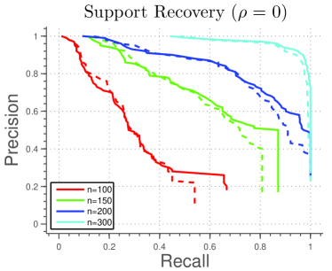
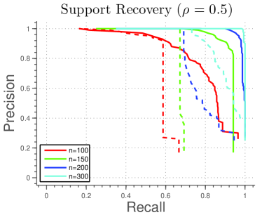
Figure 1: Precision against recall for model in Simulation 1 averaged over 100 simulation runs. Full line  () denotes results of HIPPO and dashed line  () denotes HHR.

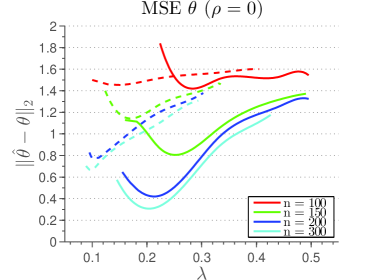
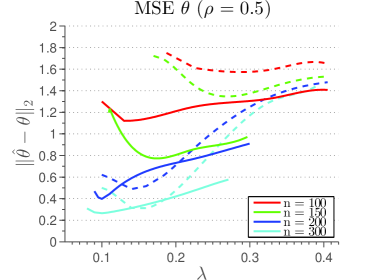
Figure 2: Error in estimating the true parameter $\theta^{\star}$ as a function of the tuning parameter $\lambda^{T}$ averaged over 100 simulation runs. Full line  () denotes results of HIPPO and dashed line  () denotes HHR.

In Simulation 1, it is assumed that the estimation procedures know the mean parameter, $\bm{\beta}={\bf 0}$ and we only estimate the variance parameter $\bm{\theta}$. This example is provided to illustrate performance of the penalized pseudolikelihood estimators in an idealized situation. When the mean parameter needs to be estimated as well, we expect the performance of the procedures only to get worse. Since the mean is known, both HHR and HIPPO only solve the optimization procedure in (4), HHR with the $\ell_{1}$-norm penalty and HIPPO with the SCAD penalty, without iterating between (5) and (4).

Figure 1 shows performance of HIPPO and HHR in identifying the support of true variance parameter $\theta^{\star}$ measured by precision and recall. Figure 2 shows $\ell_{2}$ norm between $\widehat{\theta}$ and $\theta^{\star}$ as a function of the penalty parameter. Under this toy model, we observe that HIPPO performs better than HHR.

	#it	$||\beta-\widehat{\beta}||_{2}$	${\sf Pre}_{\beta}$	${\sf Rec}_{\beta}$	$||\theta-\widehat{\theta}||_{2}$	${\sf Pre}_{\theta}$	${\sf Rec}_{\theta}$
		$n=200$
HHR-AIC	1st	0.78(0.52)	0.44(0.22)	1.00(0.00)	2.10(0.11)	0.25(0.10)	0.54(0.16)
	2nd	0.31(0.13)	0.88(0.15)	1.00(0.00)	1.80(0.16)	0.29(0.07)	0.71(0.14)
HIPPO-AIC	1st	0.66(0.84)	0.75(0.29)	1.00(0.02)	2.00(0.16)	0.20(0.10)	0.52(0.16)
	2nd	0.08(0.07)	0.84(0.24)	1.00(0.00)	1.50(0.30)	0.30(0.11)	0.75(0.12)
HHR-BIC	1st	0.77(0.48)	0.58(0.17)	1.00(0.00)	2.10(0.10)	0.41(0.18)	0.45(0.14)
	2nd	0.31(0.13)	0.89(0.13)	1.00(0.00)	1.90(0.16)	0.38(0.15)	0.65(0.17)
HIPPO-BIC	1st	0.70(0.83)	0.80(0.25)	0.99(0.03)	2.00(0.14)	0.39(0.18)	0.50(0.17)
	2nd	0.08(0.06)	0.97(0.07)	1.00(0.00)	1.60(0.28)	0.44(0.16)	0.72(0.14)
		$n=400$
HHR-AIC	1st	0.59(0.37)	0.58(0.26)	1.00(0.00)	1.90(0.11)	0.36(0.14)	0.72(0.18)
	2nd	0.30(0.24)	0.98(0.06)	1.00(0.00)	1.70(0.16)	0.43(0.13)	0.81(0.16)
HIPPO-AIC	1st	0.44(0.54)	0.87(0.22)	1.00(0.00)	1.80(0.18)	0.28(0.10)	0.67(0.15)
	2nd	0.06(0.29)	0.97(0.12)	1.00(0.02)	1.00(0.31)	0.56(0.18)	0.93(0.09)
HHR-BIC	1st	0.59(0.37)	0.66(0.20)	1.00(0.00)	1.90(0.11)	0.46(0.18)	0.66(0.20)
	2nd	0.30(0.23)	0.98(0.06)	1.00(0.00)	1.70(0.17)	0.46(0.13)	0.80(0.17)
HIPPO-BIC	1st	0.46(0.58)	0.89(0.19)	1.00(0.01)	1.80(0.18)	0.39(0.17)	0.65(0.17)
	2nd	0.06(0.29)	0.99(0.06)	1.00(0.02)	1.00(0.31)	0.63(0.20)	0.92(0.09)

Table 1: Mean (sd) performance of HHR and HIPPO under the model in Example 2 (averaged over 100 independent runs). We report estimated models after the first and second iteration.

Simulation 2. The following non-trivial model is borrowed from Daye et al. (2012). The response variable $Y$ satisfies

$$Y=\beta_{0}+\sum_{j\in[p]}X_{j}\beta_{j}+\exp(\theta_{0}+\sum_{j\in[p]}X_{j}\theta_{j})\epsilon$$

with $p=600$, $\beta_{0}=2$, $\theta_{0}=1$,

$$\bm{\beta}_{[12]}=(3,3,3,1.5,1.5,1.5,0,0,0,2,2,2)^{\prime},$$

$$\bm{\theta}_{[15]}=(1,1,1,0,0,0,0.5,0.5,0.5,0,0,0,0.75,0.75,0.75)^{\prime},$$

and the remainder of the coefficients are $0$. The covariates are jointly Normal with ${\rm cov}(X_{i},X_{j})=0.5^{|i-j|}$ and the error $\epsilon$ follows the standard Normal distribution. We set $p=600$ and change the sample size.

We first compare performance of HIPPO to an oracle procedure that knows the mean parameter $\bm{\beta}^{\star}$ or the variance parameter $\theta^{\star}$. Figure 3 shows performance of HIPPO in recovering the support of $\bm{\beta}^{\star}$ and $\bm{\theta}^{\star}$ compared to an oracle procedure. Figure 4 shows average $\ell_{2}$ norm distance between $\widehat{\bm{\theta}}$ and $\bm{\theta}^{\star}$.

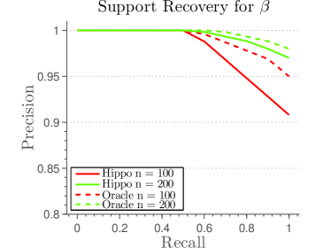
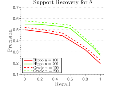
Figure 3: Precision against recall for model in Simulation 2 averaged over 100 simulation runs. The oracle procedure is assumed to know the true variance (mean) parameter $\bm{\theta}^{\star}$ $(\bm{\beta}^{\star})$ when estimating the mean (variance).

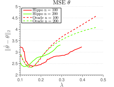
Figure 4: Error in estimating the true parameter $\theta^{\star}$ as a function of the tuning parameter $\lambda^{T}$ averaged over 100 simulation runs. The oracle procedure is assumed to know the true mean parameter $\bm{\beta}^{\star}$.

Next we compare HIPPO to HHR. Table 1 summarizes results of the simulation. We observe that HIPPO consistently outperforms HHR in all scenarios. Again, a general observation is that the AIC selects more complex models although the difference is less pronounced when the sample size $n=400$. Furthermore, we note that the estimation error significantly reduces after the first iteration, which demonstrates final sample benefits from estimating the variance. While the work of Belloni et al. (2012) shows that the first stage estimate $\widehat{\bm{\beta}}$ provides nearly-optimal MSE convergence rates, Theorem 6 proves that the third stage can achieve an optimal asymptotic variance. Hence, it is important to estimate the variance parameter $\bm{\theta}^{\star}$ well, both in theory and practice.

5 Discussion

We have analyzed the performance of HIPPO for estimating mean and variance parameters under heteroscedasticity. HIPPO is natural because it uses the lasso solution as the first stage, estimates the variances in the second stage, and then adjusts the mean parameters given the variances. The theoretical statements in Theorems 2, 4 are quite strong because they show that the HIPPO variance estimate, $\widehat{\bm{\theta}}$, attains the oracle properties under the same assumptions that are required if the true mean parameter, $\bm{\beta}^{\star}$, is known (with mild assumptions on the estimated mean parameter $\widehat{\bm{\beta}}$). A similarly strong guarantee is proven for the mean parameter in Theorem 6.

Throughout the paper, we assumed that the variance was a log-linear function of its parameters. One natural extension of this work is to estimate this function in a semi-parametric fashion, such as assuming that the log-variance has a sparse generalized additive form (as in Ravikumar et al. (2009)). HIPPO employs a non-convex penalty (for reasons stated in Section 2) and it was shown to have favorable performance in Section 4. Nonetheless, it would be of interest to see what sort of performance guarantees could be made for the lasso penalty. More generally, the heteroscedastic Gaussian model, (1), is a double generalized linear model, and extending this method to other distributions in that family would have applications in insurance and economics.

Acknowledgements

JS is supported by NSF grant DMS-1223137. This work was completed in part with resources provided by the University of Chicago Research Computing Center.

6 Appendix

6.1 Technical Lemmata

Lemma 7 (Laurent and Massart (2000)).

Let for $i\in\{1,\ldots,p\}$, $a_{i}\geq 0$ and $\{X_{i}\}_{i=1}^{p}$ be independent $\chi^{2}_{1}$ random variables. Define $Z=\sum_{i=1}^{p}a_{i}(X_{i}-1)$

$$\mathbb{P}\{Z\geq 2\|\mathbf{a}\|_{2}\sqrt{x}+2\|\mathbf{a}\|_{\infty}x\}\leq e^{-x}$$

$$\mathbb{P}\{Z\leq-2\|\mathbf{a}\|_{2}\sqrt{x}\}\leq e^{-x}$$

Specifically, this means that

$$Z=O_{\mathbb{P}}(\|\mathbf{a}\|_{1})$$

Lemma 8 (Hjort and Pollard (1993)).

Let $\ell_{n}(\bm{\theta})$ be a convex function in $t$ dimensions ($t$ possibly growing in $n$). Consider any quadratic approximation,

$$\ell_{n}(\bm{\theta}+\tilde{\bm{\theta}})=\mathbf{u}^{\prime}\tilde{\bm{\theta}}+\frac{1}{2}\tilde{\bm{\theta}}^{\prime}\mathbf{V}\tilde{\bm{\theta}}+r(\tilde{\bm{\theta}})$$

and let $\tilde{\bm{\theta}}$ denote the argmin. Let $\mathcal{A}\subset\mathbb{R}^{t}$ be compact and define the pseudo-norm

$$\|\mathbf{x}\|_{\mathcal{A}}=\sup_{\mathbf{a}\in\mathcal{A}}|\mathbf{a}^{\prime}\mathbf{x}|$$

Let the following be the difference in objectives,

$$\Delta(\delta)=\sup\{|r(\tilde{\bm{\theta}})|:\|\tilde{\bm{\theta}}-(-\mathbf{V}^{-1}\mathbf{u})\|_{\mathcal{A}}\leq\delta\}$$

Then

$$\mathbb{P}\{\|\tilde{\bm{\theta}}-(-\mathbf{V}^{-1}\mathbf{u})\|_{\mathcal{A}}\geq\delta\}\leq\mathbb{P}\{\Delta(\delta)\geq\frac{1}{2}\underline{\lambda}\delta^{2}\}$$

where

$$\underline{\lambda}=\min_{\|\mathbf{x}\|_{\mathcal{A}}=1}\mathbf{x}^{\prime}\mathbf{V}\mathbf{x}.$$

Remark 9.

This implies that if for any fixed $\delta>0$, $\Delta(\delta)=o_{\mathbb{P}}(1)$ and $\underline{\lambda}=\Omega(1)$ then

$$\|\tilde{\bm{\theta}}-(-\mathbf{V}^{-1}\mathbf{u})\|_{\mathcal{A}}=o_{\mathbb{P}}(1)$$

Proof.

This proof is based on Lemma 2 in Hjort and Pollard (1993), modified to accommodate the norm $\|.\|_{\mathcal{A}}$. ∎

Lemma 10 (Van De Geer (2000) Lemma 2.5).

A ball of radius $R$ in the Euclidean space $\mathbb{R}^{d}$ can be covered by

$$\left(\frac{4R+\delta}{\delta}\right)^{d}$$

balls of radius $\delta$.

6.2 Outline of Stage 2 Proofs

The standard procedure for constructing the local minimizer of the least squares objective with a non-convex penalty is to use the maximum likelihood estimator for likelihood with known support, $T$, and demonstrate that this achieves the first-order conditions Fan and Li (2001). Situations in which the support is known will be referred to as the oracle setting. In the known-$\bm{\beta}^{\star}$ setting (the setting of Theorem 2), we will demonstrate first that the oracle MLE where the likelihood is computed using $\widehat{\bm{\beta}}=\bm{\beta}^{\star}$ (we will refer to this estimator as the OMLE for oracle MLE) attains (12), (13), (14). Using this we will demonstrate that it gives us a local minimizer of (4), implying that it is the penalized maximum likelihood estimator (we will refer to this as the PMLE), in turn proving Theorem 2. We then consider $\widehat{\bm{\beta}}\neq\bm{\beta}^{\star}$ estimated in stage 1, and call the resulting likelihood a pseudo-likelihood. Similarly to the MLE, we show that the oracle setting for the pseudo-likelihood (we call this estimator the OMPLE) attains (12), (13), (14) under the conditions of Theorem 4 using what we have demonstrated regarding the OMLE. We then show that the OMPLE is in fact a local minimizer of the pseudo-likelihood, so that it is a penalized maximum pseudo-likelihood estimator (PMPLE), in turn proving Theorem 4. In summary, we show that the OMLE is in fact the PMLE, and then similarly demonstrate that the OMPLE is a PMPLE.

6.3 Proof of Theorem 2

Throughout this section let $\widehat{\bm{\beta}}=\bm{\beta}^{\star}$. We will begin by proving that the known-$\bm{\beta}^{\star}$ MLE, the OMLE, $\widehat{\bm{\theta}}_{T}$ attains the oracle properties. Then we will show that this is a local minimizer for (4).

6.3.1 Oracle property (14) for $\widehat{\bm{\theta}}_{T}$

Suppose that we know that the true sparsity set $T={\rm supp}(\bm{\theta}^{\star})$ and we have access to the mean parameter $\bm{\beta}^{\star}$. Thus we can determine precisely,

$$\eta^{2}_{i}=(y_{i}-\mathbf{x}_{i}^{\prime}\bm{\beta}^{\star})^{2}=\epsilon_{i}^{2}e^{\mathbf{x}_{i}^{\prime}\bm{\theta}^{\star}}.$$

Furthermore, we can minimize the likelihood for $\bm{\theta}_{T}$,

$$\ell(\bm{\theta}_{T})=\sum_{i=1}^{n}\log\sigma^{2}_{i}(\bm{\theta}_{T})+\frac{(y_{i}-\mathbf{x}_{i}^{\prime}\bm{\beta}^{\star})^{2}}{\sigma^{2}_{i}(\bm{\theta}_{T})}=\sum_{i=1}^{n}\mathbf{x}_{i,T}^{\prime}\bm{\theta}_{T}+\eta_{i}^{2}e^{-\mathbf{x}_{i,T}^{\prime}\bm{\theta}_{T}}$$

The gradient and Hessian of this log-likelihood at the true parameter $\bm{\theta}_{T}^{\star}$,

$$\mathbf{u}(\bm{\theta}_{T}^{\star})=\sum_{i=1}^{n}(1-\eta_{i}^{2}e^{-\mathbf{x}_{i,T}^{\prime}\bm{\theta}_{T}^{\star}})\mathbf{x}_{i,T}=\sum_{i=1}^{n}(1-\epsilon_{i}^{2})\mathbf{x}_{i,T}$$

$$\mathbf{V}(\bm{\theta}_{T}^{\star})=\sum_{i=1}^{n}\eta_{i}^{2}e^{-\mathbf{x}_{i,T}^{\prime}\bm{\theta}_{T}^{\star}}\mathbf{x}_{i,T}\mathbf{x}_{i,T}^{\prime}=\sum_{i=1}^{n}\epsilon_{i}^{2}\mathbf{x}_{i,T}\mathbf{x}_{i,T}^{\prime}.$$

Furthermore, the $k$-th derivative tensor of the log-likelihood is

$$\nabla^{\otimes k}\ell(\bm{\theta}_{T}^{\star})=\sum_{i=1}^{n}\eta_{i}^{2}e^{-\mathbf{x}_{i,T}^{\prime}\bm{\theta}_{T}^{\star}}\mathbf{x}_{i,T}^{\otimes k}.$$

For a tensor of the form $A=\sum_{i=1}^{n}\mathbf{a}_{i}^{\otimes k}$ and a vector $\mathbf{b}\in\mathbb{R}^{t}$ let $A(\mathbf{b})=\sum_{i=1}^{n}(\mathbf{a}^{\prime}\mathbf{b})^{k}$.

Lemma 11.

Let $k=2,3$ and

$$\widehat{\bm{\Sigma}}_{T}^{(k)}=\frac{1}{n}\sum_{i=1}^{n}\mathbf{x}_{i,T}^{\otimes k}.$$

With probability $1-\delta$, the difference between the $k$-th derivative tensor and $\widehat{\bm{\Sigma}}_{T}^{(k)}$ is bounded by

$$\Lambda_{\max}\left(\frac{1}{n}\nabla^{\otimes k}\ell(\bm{\theta}_{T}^{\star})-\widehat{\bm{\Sigma}}_{T}^{(k)}\right)\leq\frac{2}{n}\left(\sqrt{tn\Lambda_{\max}(\widehat{\bm{\Sigma}}_{T}^{(2k)})\log(\xi/\delta)}+t\max_{i\in[n]}\|\mathbf{x}_{i,T}\|^{k}\log(\xi/\delta)\right)$$

where $\xi$ is some constant only dependent on $k$.

Proof.

Let $\mathbf{a}$ be fixed such that $\|\mathbf{a}\|=1$.

$$\frac{1}{n}\nabla^{\otimes k}\ell(\bm{\theta}_{T}^{\star})-\widehat{\bm{\Sigma}}_{T}^{(k)}=\frac{1}{n}\sum_{i=1}^{n}(\epsilon_{i}^{2}-1)\mathbf{x}_{i,T}^{\otimes k}$$

$$\left(\frac{1}{n}\nabla^{\otimes k}\ell(\bm{\theta}_{T}^{\star})-\widehat{\bm{\Sigma}}_{T}^{(k)}\right)(\mathbf{a}^{\otimes k})=\frac{1}{n}\sum_{i=1}^{n}(\epsilon_{i}^{2}-1)(\mathbf{a}^{\prime}\mathbf{x}_{i,T})^{k}$$

$$\leq\frac{2}{n}\left(\sqrt{\sum_{i=1}^{n}(\mathbf{a}^{\prime}\mathbf{x}_{i,T})^{2k}\log(1/\delta)}+\max_{i\in[n]}(\mathbf{a}^{\prime}\mathbf{x}_{i,T})^{k}\log(1/\delta)\right)$$

$$\leq\frac{2}{n}\left(\sqrt{\sup_{\|\mathbf{a}\|=1}\sum_{i=1}^{n}(\mathbf{a}^{\prime}\mathbf{x}_{i,T})^{2k}\log(1/\delta)}+\max_{i\in[n]}\|\mathbf{x}_{i,T}\|^{k}\log(1/\delta)\right)$$

by Lemma 7. Let $\mathcal{A}\subset{\mathcal{S}}_{T}$ (where ${\mathcal{S}}_{T}\subset\mathbb{R}^{T}$ is the unit sphere) be a minimal $\xi$-net, meaning that for any $\mathbf{b}\in{\mathcal{S}}_{T}$, $\exists\mathbf{a}\in\mathcal{A}$ such that $\|\mathbf{a}-\mathbf{b}\|\leq\xi$ and $\mathcal{A}$ minimizes $|\mathcal{A}|$ among all such $\xi$-nets. Let $\mathbf{B}=\frac{1}{n}\nabla^{\otimes k}\ell(\bm{\theta}^{\star})-\widehat{\bm{\Sigma}}_{T}^{(k)}$. For some $\mathbf{b}\in{\mathcal{S}}_{T}$,

$$\Lambda_{\max}(\mathbf{B})=\mathbf{B}(\mathbf{b}^{\otimes k})=\mathbf{B}((\mathbf{b}^{\prime}\mathbf{a}\mathbf{a}+\sqrt{1-(\mathbf{b}^{\prime}\mathbf{a})^{2}}\mathbf{b}^{\perp})^{\otimes k})$$

where $\mathbf{a}\in\mathcal{A}$ is the closest point to $\mathbf{b}$ and $\mathbf{b}^{\perp}$ is a unit vector orthogonal to $\mathbf{a}$. Let $\xi>0$ such that

$$\left(1-\frac{\xi}{2}+\sqrt{1-(1-\xi/2)^{2}}\right)^{k}-\left(1-\frac{\xi}{2}\right)^{k}=\frac{1}{2}.$$

By assumption, $\mathbf{a}^{\prime}\mathbf{b}\geq 1-\xi/2$ ($\|\mathbf{a}-\mathbf{b}\|\leq\xi$) and

$$\mathbf{B}((\mathbf{b}^{\prime}\mathbf{a}\mathbf{a}+\sqrt{1-(\mathbf{b}^{\prime}\mathbf{a})^{2}}\mathbf{b}^{\perp})^{\otimes k})=\sum_{l=1}^{k}{k\choose l}(\mathbf{a}^{\prime}\mathbf{b})^{l}(1-(\mathbf{a}^{\prime}\mathbf{b})^{2})^{\frac{k-l}{2}}\mathbf{B}(\mathbf{a}^{\otimes l}\otimes\mathbf{b}^{\perp\otimes k-l})$$

$$\leq(\mathbf{a}^{\prime}\mathbf{b})^{k}\mathbf{B}(\mathbf{a}^{\otimes k})+\sum_{l=1}^{k-1}{k\choose l}(\mathbf{a}^{\prime}\mathbf{b})^{l}(1-(\mathbf{a}^{\prime}\mathbf{b})^{2})^{\frac{k-l}{2}}\Lambda_{\max}(\mathbf{B})\leq\mathbf{B}(\mathbf{a}^{\otimes k})+\frac{1}{2}\Lambda_{\max}(\mathbf{B}).$$

Therefore,

$$\Lambda_{\max}(\mathbf{B})\leq 2\sup_{\mathbf{a}\in\mathcal{A}}\mathbf{B}(\mathbf{a}^{\otimes k}).$$

Select $\mathcal{A}$ to be the covering of the unit ball guaranteed by Lemma 10, which is of size $C^{t}$ for some constant $C$ (since $\xi$ is a constant). Hence, we can apply the union bound by substituting $\delta\leftarrow\delta/C^{t}$, which completes the proof. ∎

Lemma 12.

Let $\delta>0$ be fixed,

$$\sup_{\tilde{\bm{\theta}}\in\mathbb{R}^{T},\|\tilde{\bm{\theta}}\|\leq\delta}\Lambda_{\max}\left(\frac{1}{n}\nabla^{\otimes 3}\ell\left(\bm{\theta}_{T}^{\star}+\frac{\sqrt{t}}{\sqrt{n}}\tilde{\bm{\theta}}\right)-\frac{1}{n}\nabla^{\otimes 3}\ell(\bm{\theta}_{T}^{\star})\right)=\tilde{o}_{\mathbb{P}}\left(t^{3/2}\right).$$

Proof.

Let $\|\mathbf{a}\|=1$,

$$\frac{1}{n}\left(\nabla^{\otimes 3}\ell(\bm{\theta}_{T}^{\star}+\frac{\sqrt{t}}{\sqrt{n}}\tilde{\bm{\theta}})-\nabla^{\otimes 3}\ell(\bm{\theta}_{T}^{\star})\right)(\mathbf{a})=\frac{1}{n}\sum_{i=1}^{n}\epsilon_{i}^{2}\left(e^{-\frac{\sqrt{t}}{\sqrt{n}}\mathbf{x}_{i,T}^{\prime}\tilde{\bm{\theta}}}-1\right)(\mathbf{x}_{i,T}^{\prime}\mathbf{a})^{3}.$$

Furthermore,

$$\left|\frac{\sqrt{t}}{\sqrt{n}}\mathbf{x}_{i,T}^{\prime}\tilde{\bm{\theta}}\right|\leq\delta\frac{\sqrt{t}}{\sqrt{n}}\max_{i\in[n]}\|\mathbf{x}_{i,T}\|=\tilde{o}(\delta t\sqrt{\log p}/\sqrt{n})=\tilde{o}(1).$$

uniformly over $\tilde{\bm{\theta}}$ by assumption (A1). Thus uniformly over $\|\mathbf{a}\|=1$,

$$\frac{1}{n}\sum_{i=1}^{n}\epsilon_{i}^{2}\left(e^{-\alpha\frac{\sqrt{t}}{\sqrt{n}}\mathbf{x}_{i,T}^{\prime}\tilde{\bm{\theta}}}-1\right)(\mathbf{x}_{i,T}^{\prime}\mathbf{a})^{3}=\tilde{o}\left((\max_{i\in[n]}\epsilon_{i}^{2})\frac{1}{n}\sum_{i=1}^{n}\|\mathbf{x}_{i,T}\|^{3}\right)=\tilde{o}_{\mathbb{P}}\left(t^{3/2}\right)$$

because $\max_{i\in[n]}|\epsilon_{i}|=\tilde{O}_{\mathbb{P}}(1)$ and by assumption (A1). ∎

We can Taylor expand the likelihood around $\bm{\theta}_{T}^{\star}$, (the mean value form where for some $\alpha\in[0,1]$)

$$\frac{1}{t}\ell\left(\bm{\theta}_{T}^{\star}+\sqrt{\frac{t}{n}}\tilde{\bm{\theta}}\right)=\frac{1}{\sqrt{tn}}\mathbf{u}(\bm{\theta}_{T}^{\star})^{\prime}\tilde{\bm{\theta}}+\frac{1}{2n}\tilde{\bm{\theta}}^{\prime}\mathbf{V}(\bm{\theta}_{T}^{\star})\tilde{\bm{\theta}}+\frac{\sqrt{t}}{6n\sqrt{n}}\left(\nabla^{\otimes 3}\ell(\bm{\theta}_{T}^{\star}+\alpha\sqrt{t/n}\tilde{\bm{\theta}})\right)(\tilde{\bm{\theta}})$$

$$\frac{1}{t}\ell\left(\bm{\theta}_{T}^{\star}+\sqrt{\frac{t}{n}}\tilde{\bm{\theta}}\right)=\frac{1}{\sqrt{tn}}\mathbf{u}(\bm{\theta}_{T}^{\star})^{\prime}\tilde{\bm{\theta}}+\frac{1}{2}\tilde{\bm{\theta}}^{\prime}\widehat{\Sigma}_{TT}\tilde{\bm{\theta}}+r(\tilde{\bm{\theta}})$$

$$\textrm{ where }r(\tilde{\bm{\theta}})=\frac{1}{2n}\tilde{\bm{\theta}}^{\prime}\left(\mathbf{V}(\bm{\theta}_{T}^{\star})-n\widehat{\Sigma}_{TT}\right)\tilde{\bm{\theta}}+\frac{\sqrt{t}}{6n\sqrt{n}}\left(\nabla^{\otimes 3}\ell(\bm{\theta}_{T}^{\star}+\alpha\sqrt{t/n}\tilde{\bm{\theta}})\right)(\tilde{\bm{\theta}}).$$

By showing that the remainder term is uniformly small, we will use the fact that if the likelihood is close to its quadratic approximation (in infinity norm) relative to their curvature of the likelihood then their optima are close. Fix $\delta>0$, set $\mathcal{A}$ to be the unit ball in $\mathbb{R}^{T}$, and define $\Delta(\delta)$ as in Lemma 8. Then under the (A1),(A2) by Lemma 11,

$$\Lambda_{\max}(\mathbf{V}(\bm{\theta}_{T}^{\star})-n\widehat{\Sigma}_{TT})=O_{\mathbb{P}}(\sqrt{tn}+t^{3/2})$$

$$\Lambda_{\max}(\nabla^{\otimes 3}\ell(\bm{\theta}_{T}^{\star})-n\widehat{\Sigma}^{(3)}_{T})=O_{\mathbb{P}}(\sqrt{nt}+t^{2}).$$

By Lemma 12,

$$\sup_{\|\tilde{\bm{\theta}}\|\leq\delta}\Lambda_{\max}(\nabla^{\otimes 3}\ell(\bm{\theta}_{T}^{\star}+\alpha\sqrt{t/n}\tilde{\bm{\theta}})-\nabla^{\otimes 3}\ell(\bm{\theta}_{T}^{\star}))=\tilde{o}_{\mathbb{P}}(t^{3/2}).$$

Further by assumption (A2),

$$\Lambda_{\max}\left(\widehat{\Sigma}_{T}^{(3)}\right)=O(1).$$

Combining these observations,

$$\Delta(\delta)=O_{\mathbb{P}}\left(\frac{\sqrt{t}}{\sqrt{n}}+\frac{t^{3/2}}{n}+\frac{t}{n}+\frac{t^{5/2}+t^{2}}{n^{3/2}}\right)=\tilde{o}_{\mathbb{P}}(1),\quad\Lambda_{\min}(\widehat{\Sigma}_{TT})=\Omega(1)$$

because $t=\tilde{o}(\sqrt{n})$.

Now let us verify that

$$\left\|\frac{1}{\sqrt{tn}}\mathbf{u}(\bm{\theta}_{T}^{\star})\right\|=O_{\mathbb{P}}(1).$$ (17)

Consider

$$\left\|\widehat{\Sigma}_{TT}^{-1}\mathbf{u}(\bm{\theta}_{T}^{\star})\right\|=\left\|\sum_{i=1}^{n}(1-\epsilon_{i}^{2})\widehat{\Sigma}^{-1}_{TT}\mathbf{x}_{i,T}\right\|.$$

By an identical argument to that used in Lemma 7,

$$\left\|\sum_{i=1}^{n}(1-\epsilon_{i}^{2})\widehat{\Sigma}^{-1}_{TT}\mathbf{x}_{i,T}\right\|=O_{\mathbb{P}}\left(\sqrt{\sum_{i=1}^{n}\|\widehat{\Sigma}_{TT}^{-1}\mathbf{x}_{i,T}\|^{2}}+\max_{i\in[n]}\|\widehat{\Sigma}_{TT}^{-1}\mathbf{x}_{i,T}\|\right)$$

$$=O_{\mathbb{P}}\left(\sqrt{\sum_{i=1}^{n}\|\mathbf{x}_{i,T}\|^{2}}+\max_{i\in[n]}\|\mathbf{x}_{i,T}\|\right)=O_{\mathbb{P}}(\sqrt{tn})$$

by (A1), (A2), and the fact that $t=\tilde{o}(\sqrt{n})$.

By Lemma 8,

$$\left\|\sqrt{\frac{n}{t}}(\widehat{\bm{\theta}}_{T}-\bm{\theta}_{T}^{\star})-\frac{1}{\sqrt{tn}}(-\widehat{\Sigma}_{TT}^{-1}\mathbf{u}(\bm{\theta}_{T}^{\star}))\right\|=o_{\mathbb{P}}(1).$$ (18)

Further, this implies that

$$\left\|\sqrt{\frac{n}{t}}(\widehat{\bm{\theta}}_{T}-\bm{\theta}_{T}^{\star})\right\|=O_{\mathbb{P}}(1).$$

6.3.2 Oracle property (12) for $\widehat{\bm{\theta}}_{T}$.

We will consider the same expansion of the likelihood as in the previous proof, except that the additional $\sqrt{t}$ factors are removed. Let $\tilde{\bm{\theta}}\in\mathbb{R}^{T}$. For some $\alpha\in[0,1]$,

$$\ell\left(\bm{\theta}_{T}^{\star}+\sqrt{\frac{1}{n}}\tilde{\bm{\theta}}\right)=\frac{1}{\sqrt{n}}\mathbf{u}(\bm{\theta}_{T}^{\star})^{\prime}\tilde{\bm{\theta}}+\frac{1}{2n}\tilde{\bm{\theta}}^{\prime}\mathbf{V}(\bm{\theta}_{T}^{\star})\tilde{\bm{\theta}}+\frac{1}{6n\sqrt{n}}\left(\nabla^{\otimes 3}\ell(\bm{\theta}_{T}^{\star}+\alpha\sqrt{t/n}\tilde{\bm{\theta}})\right)(\tilde{\bm{\theta}})$$

$$\ell\left(\bm{\theta}_{T}^{\star}+\sqrt{\frac{1}{n}}\tilde{\bm{\theta}}\right)=\frac{1}{\sqrt{n}}\mathbf{u}(\bm{\theta}_{T}^{\star})^{\prime}\tilde{\bm{\theta}}+\frac{1}{2}\tilde{\bm{\theta}}^{\prime}\widehat{\Sigma}_{TT}\tilde{\bm{\theta}}+r(\tilde{\bm{\theta}})$$

$$\textrm{ where }r(\tilde{\bm{\theta}})=\frac{1}{2n}\tilde{\bm{\theta}}^{\prime}\left(\mathbf{V}(\bm{\theta}_{T}^{\star})-n\widehat{\Sigma}_{TT}\right)\tilde{\bm{\theta}}+\frac{1}{6n\sqrt{n}}\left(\nabla^{\otimes 3}\ell(\bm{\theta}_{T}^{\star}+\alpha\sqrt{1/n}\tilde{\bm{\theta}})\right)(\tilde{\bm{\theta}}).$$

The above proof shows that $r(\tilde{\bm{\theta}})=\tilde{o}_{\mathbb{P}}(1)$ (since it proves a stronger statement) for $\|\tilde{\bm{\theta}}\|\leq\delta$. Hence, we can employ Lemma 8 with $\mathcal{A}=\{\mathbf{a}\}$ to show that,

$$\left|\sqrt{n}\mathbf{a}^{\prime}(\widehat{\bm{\theta}}-\bm{\theta}^{\star})-\frac{1}{\sqrt{n}}\left(-\mathbf{a}^{\prime}\widehat{\Sigma}^{-1}_{TT}\mathbf{u}(\bm{\theta}^{\star})\right)\right|=o_{\mathbb{P}}(1)$$

Because

$$\left|\frac{1}{\sqrt{n}}\mathbf{a}^{\prime}\mathbf{u}(\bm{\theta}^{\star})\right|=O_{\mathbb{P}}(1),\quad\underline{\lambda}=\mathbf{a}^{\prime}\widehat{\Sigma}_{TT}\mathbf{a}$$

The rest follows from the CLT.

6.3.3 Oracle property (13) for $\widehat{\bm{\theta}}_{T}$.

This is proven similarly to the previous lemmata, except with $\mathcal{A}=\{\mathbf{x}_{j,T}:j\in[n]\}$. By Lemma 7,

$$\frac{1}{\sqrt{n}}\mathbf{x}_{j,T}^{\prime}\widehat{\Sigma}_{TT}^{-1}\mathbf{u}(\bm{\theta}_{T}^{\star})=\frac{1}{\sqrt{n}}\sum_{i=1}^{n}(1-\epsilon_{i}^{2})\mathbf{x}_{j,T}^{\prime}\widehat{\Sigma}_{TT}^{-1}\mathbf{x}_{i,T}$$

$$\leq 2\left(\sqrt{\frac{1}{n}\sum_{i=1}^{n}(\mathbf{x}_{j,T}^{\prime}\widehat{\Sigma}_{TT}^{-1}\mathbf{x}_{i,T})^{2}\log(1/\delta)}+\frac{1}{\sqrt{n}}\max_{i\in[n]}|\mathbf{x}_{j,T}^{\prime}\widehat{\Sigma}_{TT}^{-1}\mathbf{x}_{i,T}|\log(1/\delta)\right)$$

$$\leq 2\left(\sqrt{\mathbf{x}_{j,T}^{\prime}\widehat{\Sigma}_{TT}^{-1}\mathbf{x}_{j,T}\log(1/\delta)}+\frac{1}{\sqrt{n}}\max_{i\in[n]}|\mathbf{x}_{j,T}^{\prime}\widehat{\Sigma}_{TT}^{-1}\mathbf{x}_{i,T}|\log(1/\delta)\right).$$

Thus, setting

$$v=\max_{j\in[n]}\left|\frac{1}{\sqrt{n}}\mathbf{x}_{j,T}^{\prime}\widehat{\Sigma}_{TT}^{-1}\mathbf{u}(\bm{\theta}_{T}^{\star})\right|=O_{\mathbb{P}}\left(\max_{j\in[n]}\sqrt{\mathbf{x}_{j,T}^{\prime}\widehat{\Sigma}_{TT}^{-1}\mathbf{x}_{j,T}\log n}+\frac{1}{\sqrt{n}}\max_{i\in[n]}|\mathbf{x}_{j,T}^{\prime}\widehat{\Sigma}_{TT}^{-1}\mathbf{x}_{i,T}|\log n\right)$$

$$=O_{\mathbb{P}}\left(\sqrt{t\log n}+\frac{t}{\sqrt{n}}\log n\right)=O_{\mathbb{P}}(\sqrt{t\log n}).$$

The above display follows from (A1) and (A2). Perform the likelihood expansion as in the previous proofs, ($\alpha\in[0,1]$)

$$\frac{1}{v^{2}}\ell\left(\bm{\theta}_{T}^{\star}+\frac{v}{\sqrt{n}}\tilde{\bm{\theta}}\right)=\frac{1}{v\sqrt{n}}\mathbf{u}(\bm{\theta}_{T}^{\star})^{\prime}\tilde{\bm{\theta}}+\frac{1}{2}\tilde{\bm{\theta}}^{\prime}\widehat{\Sigma}_{TT}\tilde{\bm{\theta}}+r(\tilde{\bm{\theta}})$$

$$\textrm{ where }r(\tilde{\bm{\theta}})=\frac{1}{2n}\tilde{\bm{\theta}}^{\prime}\left(\mathbf{V}(\bm{\theta}_{T}^{\star})-n\widehat{\Sigma}_{TT}\right)\tilde{\bm{\theta}}+\frac{v}{6n\sqrt{n}}\left(\nabla^{\otimes 3}\ell(\bm{\theta}_{T}^{\star}+\alpha\frac{\sqrt{t}}{\sqrt{n}}\tilde{\bm{\theta}})\right)(\tilde{\bm{\theta}}).$$

As in Lemma 8, set $\delta>0$, and we have that

$$\Delta(\delta)=O_{\mathbb{P}}\left(\frac{1}{2n}\Lambda_{\max}(\mathbf{V}(\bm{\theta}_{T}^{\star})-n\widehat{\Sigma}_{TT})+\frac{v}{6n\sqrt{n}}\Lambda_{\max}(\nabla^{\otimes 3}\ell(\bm{\theta}_{T}^{\star}+\alpha\frac{\sqrt{t}}{\sqrt{n}}\tilde{\bm{\theta}}))\right)$$

while $v$ is defined so that

$$\left\|\frac{1}{v\sqrt{n}}\widehat{\Sigma}^{-1}_{TT}\mathbf{u}(\bm{\theta}_{T}^{\star})\right\|_{\mathcal{A}}=O_{\mathbb{P}}(1).$$

By the proof of oracle property (12),

$$\Delta(\delta)=\tilde{o}_{\mathbb{P}}(1),\quad\Lambda_{\min}(\widehat{\Sigma}_{TT})=\Omega(1).$$

So, if $t=\tilde{o}(\sqrt{n})$, by Lemma 8,

$$\left\|\frac{\sqrt{n}}{v}(\widehat{\bm{\theta}}_{T}-\bm{\theta}_{T}^{\star})-\frac{1}{v\sqrt{n}}(-\widehat{\Sigma}_{TT}^{-1}\mathbf{u}(\bm{\theta}_{T}^{\star}))\right\|_{\mathcal{A}}=o_{\mathbb{P}}(1).$$

Hence,

$$\max_{j}\sqrt{n}|\mathbf{x}_{j,T}^{\prime}(\widehat{\bm{\theta}}_{T}-\bm{\theta}_{T}^{\star})|=O_{\mathbb{P}}(v)=O_{\mathbb{P}}\left(\max_{j\in[n]}\sqrt{\mathbf{x}_{j,T}^{\prime}\widehat{\Sigma}_{TT}^{-1}\mathbf{x}_{j,T}\log n}+\frac{1}{\sqrt{n}}\max_{i\in[n]}|\mathbf{x}_{j,T}^{\prime}\widehat{\Sigma}_{TT}^{-1}\mathbf{x}_{i,T}|\log n\right).$$

6.3.4 $\widehat{\bm{\theta}}$ is the penalized MLE.

The estimate $\widehat{\bm{\theta}}$ such that $\widehat{\bm{\theta}}_{T}$ is the OMLE (with knowledge of $T$), and $\widehat{\bm{\theta}}_{T^{C}}={\bf 0}$ is a local minimizer of (4) if the following hold (which are precisely the zero-subgradient conditions),

$$\sum_{i=1}^{n}(1-\eta_{i}^{2}e^{-\mathbf{x}_{i}^{\prime}\widehat{\bm{\theta}}})x_{i,j}-n\textrm{sgn}(\widehat{\theta}_{j})\rho^{\prime}_{\bm{\lambda}^{T}}(|\widehat{\theta}_{j}|)=0,\textrm{ if }\theta_{j}\neq 0$$ (19)

$$|\sum_{i=1}^{n}(1-\eta_{i}^{2}e^{-\mathbf{x}_{i}^{\prime}\widehat{\bm{\theta}}})x_{i,j}|<n\rho_{\bm{\lambda}^{T}}^{\prime}(0+),\textrm{ if }\theta_{j}=0.$$ (20)

We will focus on (20). Specifically, we would like to show that for $j\in T^{C}$,

$$|\sum_{i=1}^{n}(1-\eta_{i}^{2}e^{-\mathbf{x}_{i}^{\prime}\widehat{\bm{\theta}}})x_{i,j}|=o_{\mathbb{P}}\left(n\lambda^{T}_{j}\right)$$

where recall $\lambda_{j}^{T}=\lambda_{T}\|\mathbf{X}_{j}\|/n$. We can decompose this term into the following,

$$\sum_{i=1}^{n}\left(1-\eta_{i}^{2}e^{-\mathbf{x}_{i}^{\prime}\widehat{\bm{\theta}}}\right)x_{i,j}=\sum_{i=1}^{n}\left(1-\epsilon_{i}^{2}e^{-\mathbf{x}_{i}^{\prime}(\widehat{\bm{\theta}}-\bm{\theta}^{\star})}\right)x_{i,j}=\sum_{i=1}^{n}\left(1-e^{-\mathbf{x}_{i}^{\prime}(\widehat{\bm{\theta}}-\bm{\theta}^{\star})}\right)x_{i,j}+\left((1-\epsilon_{i}^{2})e^{-\mathbf{x}_{i}^{\prime}(\widehat{\bm{\theta}}-\bm{\theta}^{\star})}\right)x_{i,j}.$$

We can further decompose the second term,

$$\sum_{i=1}^{n}\left((1-\epsilon_{i}^{2})e^{-\mathbf{x}_{i}^{\prime}(\widehat{\bm{\theta}}-\bm{\theta}^{\star})}\right)x_{i,j}=\sum_{i=1}^{n}(1-\epsilon_{i}^{2})\left(e^{-\mathbf{x}_{i}^{\prime}(\widehat{\bm{\theta}}-\bm{\theta}^{\star})}-1\right)x_{i,j}+\sum_{i=1}^{n}(1-\epsilon_{i}^{2})x_{i,j}.$$

Let us label these terms,

$$A_{1}=\sum_{i=1}^{n}\left(1-e^{-\mathbf{x}_{i}^{\prime}(\widehat{\bm{\theta}}-\bm{\theta}^{\star})}\right)x_{i,j}$$

$$A_{2}=\sum_{i=1}^{n}(1-\epsilon_{i}^{2})\left(e^{-\mathbf{x}_{i}^{\prime}(\widehat{\bm{\theta}}-\bm{\theta}^{\star})}-1\right)x_{i,j}$$

$$A_{3}=\sum_{i=1}^{n}(1-\epsilon_{i}^{2})x_{i,j}.$$

Let us begin with the first term ($A_{1}$). By the mean value theorem for each $i$

$$\frac{1}{2}(\mathbf{x}_{i}^{\prime}(\widehat{\bm{\theta}}-\bm{\theta}^{\star}))^{2}e^{-|\mathbf{x}_{i}^{\prime}(\widehat{\bm{\theta}}-\bm{\theta}^{\star})|}\leq 1-e^{-\mathbf{x}_{i}^{\prime}(\widehat{\bm{\theta}}-\bm{\theta}^{\star})}-\mathbf{x}_{i}^{\prime}(\widehat{\bm{\theta}}-\bm{\theta}^{\star})\leq\frac{1}{2}(\mathbf{x}_{i}^{\prime}(\widehat{\bm{\theta}}-\bm{\theta}^{\star}))^{2}e^{|\mathbf{x}_{i}^{\prime}(\widehat{\bm{\theta}}-\bm{\theta}^{\star})|}.$$

While

$$\max_{i\in[n]}|\mathbf{x}_{i}^{\prime}(\widehat{\bm{\theta}}-\bm{\theta}^{\star})|\leq\max_{i\in[n]}\|\mathbf{x}_{i,T}\|\delta\leq\delta\sqrt{t\log p}$$

where $\delta=\|\widehat{\bm{\theta}}-\bm{\theta}^{\star}\|=O_{\mathbb{P}}(\sqrt{t/n})$ by (14). Hence,

$$\max_{i\in[n]}|\mathbf{x}_{i}^{\prime}(\widehat{\bm{\theta}}-\bm{\theta}^{\star})|=o_{\mathbb{P}}(1).$$ (21)

Therefore, uniformly over $j\in T^{C}$,

$$\sum_{i=1}^{n}\left(1-e^{-\mathbf{x}_{i}^{\prime}(\widehat{\bm{\theta}}-\bm{\theta}^{\star})}\right)x_{i,j}=\sum_{i=1}^{n}\mathbf{x}_{i}^{\prime}(\widehat{\bm{\theta}}-\bm{\theta}^{\star})x_{i,j}+\left(\frac{1}{2}\sum_{i=1}^{n}(\mathbf{x}_{i}^{\prime}(\widehat{\bm{\theta}}-\bm{\theta}^{\star}))^{2}x_{i,j}\right)(1+o_{\mathbb{P}}(1)).$$

We will first bound the term

$$\sum_{i=1}^{n}\mathbf{x}_{i}^{\prime}(\widehat{\bm{\theta}}-\bm{\theta}^{\star})\frac{x_{i,j}}{\|\mathbf{X}_{j}\|}.$$

Define the following

$$\mathbf{b}=\frac{1}{n}\sum_{i=1}^{n}(\epsilon_{i}^{2}-1)\widehat{\Sigma}_{TT}^{-1}\mathbf{x}_{i,T}$$

then we have that

$$\|(\widehat{\bm{\theta}}-\bm{\theta})-\mathbf{b}\|=O_{\mathbb{P}}(\sqrt{t/n})$$

by (18). Let $\bm{\alpha}_{j}=\mathbf{X}_{j}/\|\mathbf{X}_{j}\|$, then by Cauchy-Schwartz

$$\max_{j\in T^{C}}\left|\sum_{i=1}^{n}\mathbf{x}_{i}^{\prime}(\widehat{\bm{\theta}}-\bm{\theta}^{\star})\alpha_{j,i}-n^{-1}\sum_{i_{1},i_{2}=1}^{n}\alpha_{j,i_{1}}(\epsilon_{i_{2}}^{2}-1)\mathbf{x}_{i_{1},T}^{\prime}\widehat{\Sigma}_{TT}^{-1}\mathbf{x}_{i_{2},T}\right|$$

$$\leq\max_{j\in T^{C}}\|(\widehat{\bm{\theta}}-\bm{\theta})-\mathbf{b}\|\|\mathbf{X}_{T}\bm{\alpha}_{j}\|=\tilde{O}_{\mathbb{P}}(n^{1/4}\sqrt{t/n})=\tilde{o}_{\mathbb{P}}(1)$$

by (11) and the fact that $t=\tilde{o}(\sqrt{n})$. Define

$$\mathbf{P}_{T}=\mathbf{X}_{T}^{\prime}(\mathbf{X}_{T}\mathbf{X}_{T}^{\prime})^{-1}\mathbf{X}_{T}$$

so that

$$n^{-1}\sum_{i_{1},i_{2}=1}^{n}\alpha_{j,i_{1}}(\epsilon_{i_{2}}^{2}-1)\mathbf{x}_{i_{1},T}^{\prime}\widehat{\Sigma}_{TT}^{-1}\mathbf{x}_{i_{2},T}=(\bm{\epsilon}^{2}-{\bf 1})^{\prime}\mathbf{P}_{T}\bm{\alpha}_{j}$$

and

$$\max_{j\in T^{C}}|(\bm{\epsilon}^{2}-{\bf 1})^{\prime}\mathbf{P}_{T}\bm{\alpha}_{j}|=O_{\mathbb{P}}\left(\max_{j\in T^{C}}\|\mathbf{P}_{T}\bm{\alpha}_{j}\|\sqrt{\log p}\right)+O_{\mathbb{P}}\left(\max_{j\in T^{C}}\|\mathbf{P}_{T}\bm{\alpha}_{j}\|_{\infty}\log p\right)$$

by Lemma 7 combined with the union bound. Considering the first term, we have

$$\max_{j\in T^{C}}\left\|\mathbf{P}_{T}\bm{\alpha}_{j}\right\|=n^{-1/2}\Lambda_{\max}(\widehat{\Sigma}_{TT}^{-1/2})\max_{j\in T^{C}}\|\mathbf{X}_{T}\bm{\alpha}_{j}\|=\tilde{O}_{\mathbb{P}}(n^{-1/4})=\tilde{o}_{\mathbb{P}}(1)$$

by (11) and (A2). Considering the second term,

$$\max_{j\in T^{C}}\|\mathbf{P}_{T}\bm{\alpha}_{j}\|_{\infty}\leq\max_{j\in T^{C}}\|\mathbf{P}_{T}\bm{\alpha}_{j}\|=\tilde{o}(1).$$

Hence,

$$\left|\sum_{i=1}^{n}\mathbf{x}_{i}^{\prime}(\widehat{\bm{\theta}}-\bm{\theta}^{\star})\frac{x_{i,j}}{\|\mathbf{X}_{j}\|}\right|=\tilde{o}_{\mathbb{P}}(1).$$ (22)

Furthermore, by (12)

$$\max_{i\in[n]}|\mathbf{x}_{i}^{\prime}(\widehat{\bm{\theta}}-\bm{\theta}^{\star})|=\tilde{O}_{\mathbb{P}}(\sqrt{t/n})$$

and so

$$\sum_{i=1}^{n}(\mathbf{x}_{i}^{\prime}(\widehat{\bm{\theta}}-\bm{\theta}^{\star}))^{2}\frac{x_{i,j}}{\|\mathbf{X}_{j}\|}\leq\sqrt{n}\max_{i\in[n]}|\mathbf{x}_{i}^{\prime}(\widehat{\bm{\theta}}-\bm{\theta}^{\star})|^{2}=\tilde{O}_{\mathbb{P}}(t/\sqrt{n})=o_{\mathbb{P}}(1).$$

In conclusion, $A_{1}/\|\mathbf{X}_{j}\|=o_{\mathbb{P}}(\sqrt{\log n})$ uniformly in $j\in T^{C}$.

Focusing on the term $A_{3}$, by Lemma 7 and the union bound,

$$\sup_{j\in T^{C}}\sum_{i=1}^{n}(1-\epsilon_{i}^{2})\alpha_{i,j}=O_{\mathbb{P}}\left(\sqrt{\sum_{i=1}^{n}\alpha_{i,j}^{2}\log p}+\max_{i,j}|\alpha_{i,j}|\log p\right).$$

Because $\max_{i,j}\alpha_{i,j}=O(\log^{-1/2}p)$, $A_{3}=O_{\mathbb{P}}(\sqrt{\log p})$.

We now focus on $A_{2}$. Let $\delta>0$ depend on $n$, such that $\delta=O(\sqrt{t/n})$ and $\mathbb{P}\{\|\widehat{\bm{\theta}}-\bm{\theta}^{\star}\|>\delta\}\leq\eta_{0}$ for some fixed $\eta_{0}>0$. By the mean value theorem,

$$\max_{i\in[n]}\left|e^{-\mathbf{x}_{i}^{\prime}(\widehat{\bm{\theta}}-\bm{\theta}^{\star})}-1\right|\leq\max_{i\in[n]}|\mathbf{x}_{i}^{\prime}(\widehat{\bm{\theta}}-\bm{\theta}^{\star})|e^{|\mathbf{x}_{i}^{\prime}(\widehat{\bm{\theta}}-\bm{\theta}^{\star})|}=O_{\mathbb{P}}(\delta\sqrt{t\log n})$$

since by (21), $e^{|\mathbf{x}_{i}^{\prime}(\widehat{\bm{\theta}}-\bm{\theta}^{\star})|}=1+o_{\mathbb{P}}(1)$. We will provide a covering argument that controls,

$$f_{j}(\bm{\theta})=\sum_{i=1}^{n}(1-\epsilon_{i}^{2})\left(e^{-\mathbf{x}_{i}^{\prime}(\widehat{\bm{\theta}}-\bm{\theta}^{\star})}-1\right)\frac{x_{i,j}}{\|\mathbf{X}_{j}\|}$$

uniformly over $j\in T^{C}$ and $\Theta=\{\bm{\theta}\in\mathbb{R}^{T}:\|\bm{\theta}-\bm{\theta}^{\star}\|\leq\delta\}$. Define $\alpha_{i,j}=x_{i,j}/\|\mathbf{X}_{j}\|$. Consider a pair $\bm{\theta}_{0},\bm{\theta}_{1}\in\Theta$,

$$\max_{j\in T^{C}}|f_{j}(\bm{\theta}_{0})-f_{j}(\bm{\theta}_{1})|\leq\max_{j\in T^{C}}\left|\sum_{i=1}^{n}(1-\epsilon_{i}^{2})\left(e^{-\mathbf{x}_{i}^{\prime}(\bm{\theta}_{0}-\bm{\theta}^{\star})}-e^{-\mathbf{x}_{i}^{\prime}(\bm{\theta}_{1}-\bm{\theta}^{\star})}\right)\alpha_{i,j}\right|$$

$$\leq\left(\max_{j\in T^{C}}\sum_{i=1}^{n}|1-\epsilon_{i}^{2}||\alpha_{i,j}|\right)\max_{i\in[n]}\left|e^{-\mathbf{x}_{i}^{\prime}(\bm{\theta}_{0}-\bm{\theta}^{\star})}-e^{-\mathbf{x}_{i}^{\prime}(\bm{\theta}_{1}-\bm{\theta}^{\star})}\right|.$$

Now consider balls of radius $\gamma$, and let $a=\max_{i\in[n]}\|\mathbf{x}_{i,T}\|\delta$, then by the mean value theorem,

$$\sup_{\|\bm{\theta}_{0}-\bm{\theta}_{1}\|\leq\gamma}\max_{i\in[n]}\left|e^{-\mathbf{x}_{i}^{\prime}(\bm{\theta}_{0}-\bm{\theta}^{\star})}-e^{-\mathbf{x}_{i}^{\prime}(\bm{\theta}_{1}-\bm{\theta}^{\star})}\right|\leq\sup_{\|\bm{\theta}_{0}-\bm{\theta}_{1}\|\leq\gamma}\max_{i\in[n]}e^{|\mathbf{x}_{i}^{\prime}(\bm{\theta}_{1}-\bm{\theta}^{\star})|}\left|e^{\mathbf{x}_{i}^{\prime}(\bm{\theta}_{1}-\bm{\theta}_{0})}-1\right|$$

$$=e^{a}\sup_{\|\bm{\theta}_{0}-\bm{\theta}_{1}\|\leq\gamma}\max_{i\in[n]}|\mathbf{x}_{i}^{\prime}(\bm{\theta}_{1}-\bm{\theta}_{0})|e^{|\mathbf{x}_{i}^{\prime}(\bm{\theta}_{1}-\bm{\theta}_{0})|}\leq e^{3a}\gamma\max_{i\in[n]}\|\mathbf{x}_{i,T}\|=O(\gamma\sqrt{t\log n})$$

because we have shown that $a=o(1)$. By Cauchy-Schwartz and the LLN,

$$\max_{j\in T^{C}}\sum_{i=1}^{n}|1-\epsilon_{i}^{2}||\alpha_{i,j}|\leq\sqrt{\sum_{i=1}^{n}(1-\epsilon_{i}^{2})^{2}}=O_{\mathbb{P}}(\sqrt{n}).$$

By assumption (A1) if $\gamma=o((\sqrt{tn\log n})^{-1})$, then

$$\sup_{\|\bm{\theta}_{0}-\bm{\theta}_{1}\|\leq\gamma}\max_{j\in T^{C}}|f_{j}(\bm{\theta}_{0})-f_{j}(\bm{\theta}_{1})|=o_{\mathbb{P}}(1)$$

Now we know that we can cover $\Theta$ with an entropy of $O(t\log n)$ by Lemma 10. For each center in the covering ($\bm{\theta}$), with probability $\eta>0$, by Lemma 7,

$$f_{j}(\bm{\theta})=\sum_{i=1}^{n}(1-\epsilon_{i}^{2})\left(e^{-\mathbf{x}_{i}^{\prime}(\bm{\theta}-\bm{\theta}^{\star})}-1\right)x_{i,j}$$

$$\leq 2\sqrt{\sum_{i=1}^{n}\left(e^{-\mathbf{x}_{i}^{\prime}(\bm{\theta}-\bm{\theta}^{\star})}-1\right)^{2}\alpha_{i,j}^{2}\log(1/\eta)}+2\max_{i\in[n]}\left|e^{-\mathbf{x}_{i}^{\prime}(\bm{\theta}-\bm{\theta}^{\star})}-1\right||\alpha_{i,j}|\log(1/\eta)$$

$$\leq 4\max_{i\in[n]}\left|e^{-\mathbf{x}_{i}^{\prime}(\bm{\theta}-\bm{\theta}^{\star})}-1\right|\left(\sqrt{\log(1/\eta)}+\max_{i,j}|\alpha_{i,j}|\log(1/\eta)\right).$$

We have that the convergence in (21) is uniform over $\widehat{\bm{\theta}}\in\Theta$, so

$$\sup_{\bm{\theta}\in\Theta}|e^{-\mathbf{x}_{i}^{\prime}(\bm{\theta}-\bm{\theta}^{\star})}-1|=O\left(\max_{i\in[n]}\sup_{\bm{\theta}\in\Theta}|\mathbf{x}_{i}^{\prime}(\bm{\theta}-\bm{\theta}^{\star})|\right)=O_{\mathbb{P}}(\sqrt{t\log n}/\sqrt{n}).$$

Recall that we have assumed that $\max_{i,j}|\alpha_{i,j}|=\tilde{o}(n^{1/2}/t^{3/2})$ and $\log p=\tilde{O}(1)$. Setting $\eta$ such that $\log(1/\eta)\propto t\log n+\log p$ then

$$\max_{j\in[p]}\sup_{\bm{\theta}}f_{j}(\bm{\theta})=\tilde{O}_{\mathbb{P}}\left(\sqrt{\frac{t\log n}{n}}\left(\sqrt{t\log n}+\tilde{o}\left(\frac{\sqrt{n}}{t\sqrt{t}}\right)t\log n\right)\right)=\tilde{O}_{\mathbb{P}}\left(\frac{t}{\sqrt{n}}+\frac{t^{2}}{n}\right)=\tilde{o}_{\mathbb{P}}(1)$$

where the supremum in $\bm{\theta}$ is over the cover centers. Because this is higher order than the differences within balls in the cover, we have that

$$\max_{j\in[p]}\sup_{\bm{\theta}\in\bm{\Theta}}f_{j}(\bm{\theta})=o_{\mathbb{P}}(\sqrt{\log p})$$

because $\eta_{0}$ (which was a function of $\delta$) can be set to be arbitrarily small. In conclusion $A_{3}/\|\mathbf{X}_{j}\|=o_{\mathbb{P}}(\sqrt{\log p})$ uniformly in $j$, which implies (20) for $\lambda_{T}=\omega(\sqrt{\log p})$.

In order to show (19), we can demonstrate that

$$\|\widehat{\bm{\theta}}_{T}-\bm{\theta}^{\star}_{T}\|_{\infty}=O_{\mathbb{P}}\left(\sqrt{\frac{\log p}{n}}\right)$$

by identical procedures to the proofs of (12), (13), (14) . Furthermore, for $j\in T$,

$$\Lambda_{\min}(\widehat{\Sigma}_{TT})\leq n^{-1}\|\mathbf{X}_{j}\|^{2}\leq\Lambda_{\max}(\widehat{\Sigma}_{TT}).$$

Hence, if

$$\theta^{\star}_{j}=\omega\left(\frac{\sqrt{\log p}}{\sqrt{n}}\right),\quad\forall j\in T$$

then

$$\widehat{\theta}_{j}=\omega\left(\frac{\sqrt{\log p}}{\sqrt{n}}\right)=\omega\left(\frac{\sqrt{\log p}}{n}\|\mathbf{X}_{j}\|\right),\quad\forall j\in T$$

and there is a sequence $\lambda_{T}$ such that (19) holds. This demonstrates that $\widehat{\bm{\theta}}$ is the PMLE.

6.4 Proof of Theorem 4

We now consider $\widehat{\bm{\beta}}\neq\bm{\beta}^{\star}$, but rather it satisfies (15). We will analyze the oracle pseudo-likelihood setting (the OMPLE). Throughout this section, we will make the following assumption about the performance of stage 1

$$\widehat{\bm{\beta}}\in\mathcal{B}=\{\bm{\beta}\in\mathbb{R}^{p}:\|\bm{\beta}\|_{0}\leq\widehat{s},\|\mathbf{X}(\bm{\beta}^{\star}-\bm{\beta})\|^{2}\leq r\}$$ (23)

for some $\widehat{s}=\tilde{o}(\sqrt{n})$ and $r=O(\widehat{s})$ as is guaranteed by (15). The negative log-likelihood and negative log-pseudo-likelihood are given by

$$\ell(\bm{\theta})= \sum_{i=1}^{n}\log\sigma_{i}(\bm{\theta})^{2}+\frac{(y_{i}-\mathbf{x}_{i}^{\prime}\bm{\beta})^{2}}{\sigma_{i}(\bm{\theta})^{2}}=\sum_{i=1}^{n}\log\sigma_{i}(\bm{\theta})^{2}+\epsilon_{i}^{2}e^{\mathbf{x}_{i}^{\prime}(\bm{\theta}^{\star}-\bm{\theta})}$$

$$\widehat{\ell}(\bm{\theta})= \sum_{i=1}^{n}\log\sigma_{i}(\bm{\theta})^{2}+\frac{(y_{i}-\mathbf{x}_{i}^{\prime}\widehat{\bm{\beta}})^{2}}{\sigma_{i}(\bm{\theta})^{2}}=\sum_{i=1}^{n}\log\sigma_{i}(\bm{\theta})^{2}+\epsilon_{i}^{2}e^{\mathbf{x}_{i}^{\prime}(\bm{\theta}^{\star}-\bm{\theta})}$$

$$+(\mathbf{x}_{i}^{\prime}(\bm{\beta}^{\star}-\widehat{\bm{\beta}}))^{2}e^{-\mathbf{x}_{i}^{\prime}\bm{\theta}}+2\epsilon_{i}\mathbf{x}_{i}^{\prime}(\widehat{\bm{\beta}}-\bm{\beta})e^{\frac{1}{2}\mathbf{x}_{i}^{\prime}(\bm{\theta}^{\star}-\bm{\theta})}$$

We will augment the pseudo-likelihood by introducing constants in $\bm{\theta}$ which does not affect the minimizer,

$$\widehat{\ell}^{\prime}(\bm{\theta})=\sum_{i=1}^{n}\log\sigma_{i}(\bm{\theta})^{2}+\frac{(y_{i}-\mathbf{x}_{i}^{\prime}\widehat{\bm{\beta}})^{2}}{\sigma_{i}(\bm{\theta})^{2}}=\sum_{i=1}^{n}\log\sigma_{i}(\bm{\theta})^{2}+\epsilon_{i}^{2}e^{\mathbf{x}_{i}^{\prime}(\bm{\theta}^{\star}-\bm{\theta})}$$

$$+(\mathbf{x}_{i}^{\prime}(\bm{\beta}^{\star}-\widehat{\bm{\beta}}))^{2}\left(e^{-\mathbf{x}_{i}^{\prime}\bm{\theta}}-e^{-\mathbf{x}_{i}^{\prime}\bm{\theta}^{\star}}\right)+2\epsilon_{i}\mathbf{x}_{i}^{\prime}(\widehat{\bm{\beta}}-\bm{\beta})\left(e^{\frac{1}{2}\mathbf{x}_{i}^{\prime}(\bm{\theta}^{\star}-\bm{\theta})}-1\right).$$

Lemma 13.

Let $C>0$ and define

$$\Theta_{C}=\left\{\bm{\theta}\in\mathbb{R}^{T}:\|\mathbf{X}(\bm{\theta}-\bm{\theta}^{\star})\|_{\infty}\leq C\sqrt{\frac{t}{n}\log n},\|\bm{\theta}-\bm{\theta}^{\star}\|\leq C\sqrt{\frac{t}{n}}\right\}$$

Then the likelihood difference is bounded by

$$\sup_{\bm{\theta}\in\Theta_{C}}|\widehat{\ell}^{\prime}(\bm{\theta})-\ell(\bm{\theta})|=o_{\mathbb{P}}(t)$$

Proof.

The difference is

$$\widehat{\ell}^{\prime}(\bm{\theta})-\ell(\bm{\theta})=\sum_{i=1}^{n}(\mathbf{x}_{i}^{\prime}(\bm{\beta}^{\star}-\widehat{\bm{\beta}}))^{2}\left(e^{-\mathbf{x}_{i}^{\prime}\bm{\theta}}-e^{-\mathbf{x}_{i}^{\prime}\bm{\theta}^{\star}}\right)+2\epsilon_{i}\mathbf{x}_{i}^{\prime}(\widehat{\bm{\beta}}-\bm{\beta})\left(e^{\frac{1}{2}\mathbf{x}_{i}^{\prime}(\bm{\theta}^{\star}-\bm{\theta})}-1\right).$$ (24)

The first term will be controlled later by a perturbation arguments while the second term requires a covering argument. Consider the second term of (24),

$$f(\bm{\theta},\widehat{\bm{\beta}})=\sum_{i=1}^{n}\epsilon_{i}\mathbf{x}_{i}^{\prime}(\widehat{\bm{\beta}}-\bm{\beta}^{\star})\left(e^{\frac{1}{2}\mathbf{x}_{i}^{\prime}(\bm{\theta}^{\star}-\bm{\theta})}-1\right)$$

as a function of $\bm{\theta},\widehat{\bm{\beta}}$. We are trying to argue that for any $\bm{\theta}\in\Theta$ and $\widehat{\bm{\beta}}\in\mathcal{B}$, $f(\bm{\theta},\widehat{\bm{\beta}})$ is small. Let $\bm{\theta}_{0},\bm{\theta}_{1}\in\Theta$ and $\bm{\beta}_{0},\bm{\beta}_{1}\in\mathcal{B}$.

$$|f(\bm{\theta}_{0},\bm{\beta}_{0})-f(\bm{\theta}_{1},\bm{\beta}_{1})|=\left|\sum_{i=1}^{n}\epsilon_{i}\left(\mathbf{x}_{i}^{\prime}(\bm{\beta}_{0}-\bm{\beta}^{\star})e^{\frac{1}{2}\mathbf{x}_{i}^{\prime}(\bm{\theta}^{\star}-\bm{\theta}_{0})}-\mathbf{x}_{i}^{\prime}(\bm{\beta}_{1}-\bm{\beta}^{\star})e^{\frac{1}{2}\mathbf{x}_{i}^{\prime}(\bm{\theta}^{\star}-\bm{\theta}_{1})}+\mathbf{x}_{i}^{\prime}(\bm{\beta}_{0}-\bm{\beta}_{1})\right)\right|$$

$$\leq\|\bm{\epsilon}\|\sqrt{\sum_{i=1}^{n}\left(\mathbf{x}_{i}^{\prime}(\bm{\beta}_{0}-\bm{\beta}^{\star})e^{\frac{1}{2}\mathbf{x}_{i}^{\prime}(\bm{\theta}^{\star}-\bm{\theta}_{0})}-\mathbf{x}_{i}^{\prime}(\bm{\beta}_{1}-\bm{\beta}^{\star})e^{\frac{1}{2}\mathbf{x}_{i}^{\prime}(\bm{\theta}^{\star}-\bm{\theta}_{1})}\right)^{2}}+\|\bm{\epsilon}\|\|\mathbf{X}(\bm{\beta}_{0}-\bm{\beta}_{1})\|$$

Consider two pairs, $\bm{\delta}_{0}=\bm{\beta}^{\star}-\bm{\beta}_{0},\bm{\delta}_{1}=\bm{\beta}^{\star}-\bm{\beta}_{1}$ and $\bm{\theta}_{0},\bm{\theta}_{1}\in\Theta$ and consider the difference in objectives,

$$\left|\mathbf{x}_{i}^{\prime}\bm{\delta}_{0}e^{\frac{1}{2}\mathbf{x}_{i}^{\prime}(\bm{\theta}^{\star}-\bm{\theta}_{0})}-\mathbf{x}_{i}^{\prime}\bm{\delta}_{1}e^{\frac{1}{2}\mathbf{x}_{i}^{\prime}(\bm{\theta}^{\star}-\bm{\theta}_{1})}\right|$$

$$\leq\left|\mathbf{x}_{i}^{\prime}\bm{\delta}_{0}\left(e^{\frac{1}{2}\mathbf{x}_{i}^{\prime}(\bm{\theta}^{\star}-\bm{\theta}_{0})}-e^{\frac{1}{2}\mathbf{x}_{i}^{\prime}(\bm{\theta}^{\star}-\bm{\theta}_{1})}\right)\right|+\left|\mathbf{x}_{i}^{\prime}(\bm{\delta}_{0}-\bm{\delta}_{1})e^{\frac{1}{2}\mathbf{x}_{i}^{\prime}(\bm{\theta}^{\star}-\bm{\theta}_{1})}\right|$$

$$\leq\frac{1}{2}|\mathbf{x}_{i}^{\prime}\bm{\delta}_{0}|\|\mathbf{x}_{i,T}\|\|\bm{\theta}_{0}-\bm{\theta}_{1}\|e^{\frac{1}{2}\mathbf{x}_{i}^{\prime}(\bm{\theta}^{\star}-\tilde{\bm{\theta}}_{i})}+\left|\mathbf{x}_{i}^{\prime}(\bm{\delta}_{0}-\bm{\delta}_{1})\right|e^{\frac{1}{2}\mathbf{x}_{i}^{\prime}(\bm{\theta}^{\star}-\bm{\theta}_{1})}$$

for some $\tilde{\bm{\theta}}_{i}$ on the segment between $\bm{\theta}_{1}$ and $\bm{\theta}_{0}$ by the mean value theorem. Assume that $\|\mathbf{X}(\bm{\delta}_{0}-\bm{\delta}_{1})\|\leq\gamma_{\beta}$. Assume that $\|\bm{\theta}_{0}-\bm{\theta}_{1}\|\leq\gamma_{\theta}$, and define $\overline{\sigma}^{2}(\Theta)=\max_{\bm{\theta}\in\Theta}\max_{i}e^{\mathbf{x}_{i}^{\prime}(\bm{\theta}^{\star}-\bm{\theta})}$,

$$\sum_{i=1}^{n}\left|\mathbf{x}_{i}^{\prime}\bm{\delta}_{0}e^{\frac{1}{2}\mathbf{x}_{i}^{\prime}(\bm{\theta}^{\star}-\bm{\theta}_{0})}-\mathbf{x}_{i}^{\prime}\bm{\delta}_{1}e^{\frac{1}{2}\mathbf{x}_{i}^{\prime}(\bm{\theta}^{\star}-\bm{\theta}_{1})}\right|^{2}$$

$$\leq\sum_{i=1}^{n}\frac{\gamma_{\theta}^{2}}{2}(\mathbf{x}_{i}^{\prime}\bm{\delta}_{0})^{2}\|\mathbf{x}_{i,T}\|^{2}e^{\mathbf{x}_{i}^{\prime}(\bm{\theta}^{\star}-\tilde{\bm{\theta}}_{i})}+2\left(\mathbf{x}_{i}^{\prime}(\bm{\delta}_{0}-\bm{\delta}_{1})\right)^{2}e^{\mathbf{x}_{i}^{\prime}(\bm{\theta}^{\star}-\bm{\theta}_{1})}$$

$$\leq\frac{\gamma_{\theta}^{2}}{2}\left(\max_{i}\|\mathbf{x}_{i,T}\|^{2}\max_{\tilde{\bm{\theta}}_{i}}e^{\mathbf{x}_{i}^{\prime}(\bm{\theta}^{\star}-\tilde{\bm{\theta}}_{i})}\right)\|\mathbf{X}\bm{\delta}_{0}\|^{2}+2\|\mathbf{X}(\bm{\delta}_{0}-\bm{\delta}_{1})\|^{2}\max_{i}e^{\mathbf{x}_{i}^{\prime}(\bm{\theta}^{\star}-\bm{\theta}_{1})}$$

$$\leq r\overline{\sigma}^{2}(\Theta)\frac{\gamma_{\theta}^{2}}{2}|\!|\!|\mathbf{X}_{T}|\!|\!|_{{2,\infty}}^{2}+2\gamma_{\beta}^{2}\overline{\sigma}^{2}(\Theta)=o(rt\gamma_{\theta}^{2}\log n)+o(\gamma_{\beta}^{2})$$

uniformly over such pairs ($\bm{\theta}_{0},\bm{\theta}_{1},\bm{\beta}_{0},\bm{\beta}_{1}$) by (A1) and the fact that $\overline{\sigma}(\Theta)=1+o(1)$ (by similar reasoning as in the previous proofs). Thus, if

$$\gamma^{2}_{\theta}=O\left((rt\log n)^{-1}n^{-1/2}\right),\quad\gamma^{2}_{\beta}=O(n^{-1/2})$$

then

$$\sup_{\|\bm{\theta}_{0}-\bm{\theta}_{1}\|\leq\gamma_{\theta},\|\mathbf{X}(\bm{\delta}_{0}-\bm{\delta}_{1})\|_{2}\leq\gamma_{\beta}}\sum_{i=1}^{n}\left|\mathbf{x}_{i}^{\prime}\bm{\delta}_{0}e^{\frac{1}{2}\mathbf{x}_{i}^{\prime}(\bm{\theta}^{\star}-\bm{\theta}_{0})}-\mathbf{x}_{i}^{\prime}\bm{\delta}_{1}e^{\frac{1}{2}\mathbf{x}_{i}^{\prime}(\bm{\theta}^{\star}-\bm{\theta}_{1})}\right|^{2}=o(n^{-1/2})$$

as well as $\|\mathbf{X}(\bm{\beta}_{0}-\bm{\beta}_{1})\|=o(n^{-1/2})$. These conditions are satisfied by

$$\gamma_{\theta}=n^{-2},\quad\gamma_{\beta}=n^{-1}.$$

We are able to cover the space $\mathcal{B}$ with $e^{O(\widehat{s}\log p)}$ balls of radius $n^{-1}$. We also can cover the space $\Theta$ with $e^{O(t\log p)}$ of radius $n^{-2}$, hence the metric entropy, $\log N(\gamma)$, is bounded by

$$\log N(\gamma)=O\left((\widehat{s}+t)\log p\ \right).$$

For a fixed $\widehat{\bm{\beta}}$ and $\bm{\theta}$, by Gaussian concentration with probability $1-\eta$,

$$f(\bm{\theta},\widehat{\bm{\beta}})=\sum_{i=1}^{n}\epsilon_{i}\mathbf{x}_{i}^{\prime}(\widehat{\bm{\beta}}-\bm{\beta}^{\star})\left(e^{\frac{1}{2}\mathbf{x}_{i}^{\prime}(\bm{\theta}^{\star}-\bm{\theta})}-1\right)$$

$$\leq\sqrt{2\sum_{i=1}^{n}(\mathbf{x}_{i}^{\prime}(\bm{\beta}^{\star}-\widehat{\bm{\beta}}))^{2}\left(e^{\frac{1}{2}\mathbf{x}_{i}^{\prime}(\bm{\theta}^{\star}-\bm{\theta})}-1\right)^{2}\log(1/\eta)}.$$

Setting $\eta\propto N(\gamma)^{-1}$ (it can be shown that the first term is dominating based on (A1)),

$$\sup_{\bm{\theta}\in\Theta,\widehat{\bm{\beta}}\in\mathcal{B}}f(\bm{\theta},\widehat{\bm{\beta}})=O_{\mathbb{P}}\left(\|\mathbf{X}(\bm{\beta}^{\star}-\widehat{\bm{\beta}})\|\sqrt{\frac{t\log n}{n}}\sqrt{(\widehat{s}+t)\log p}\right)=\tilde{o}_{\mathbb{P}}(t)$$

by the fact that $r,s,t=\tilde{o}(\sqrt{n})$ and $\log p=\tilde{O}(1)$. The first term in the likelihood difference, (24), is bounded by

$$\|\mathbf{X}(\bm{\beta}^{\star}-\widehat{\bm{\beta}})\|^{2}\sup_{\bm{\theta}\in\Theta}\max_{i\in[n]}\left|e^{-\mathbf{x}_{i}^{\prime}\bm{\theta}}-e^{-\mathbf{x}_{i}^{\prime}\bm{\theta}^{\star}}\right|\leq\underline{\sigma}^{-2}\|\mathbf{X}(\bm{\beta}^{\star}-\widehat{\bm{\beta}})\|^{2}\sup_{\bm{\theta}\in\Theta}\max_{i\in[n]}\left|e^{\mathbf{x}_{i}^{\prime}(\bm{\theta}^{\star}-\bm{\theta})}-1\right|$$

$$\leq\tilde{O}_{\mathbb{P}}\left(\underline{\sigma}^{-2}\|\mathbf{X}(\bm{\beta}^{\star}-\widehat{\bm{\beta}})\|^{2}\sqrt{\frac{t\log n}{n}}\right)=o_{\mathbb{P}}(\sqrt{t})$$

where $\underline{\sigma}=\min_{i}\sigma_{i}$ so that $\underline{\sigma}^{-2}=\tilde{O}(1)$. ∎

(13) and (A1) imply

$$\max_{i,j\in[n]}\sqrt{\mathbf{x}_{j,T}^{\prime}\widehat{\Sigma}_{TT}^{-1}\mathbf{x}_{i,T}}=O\left(\|\mathbf{X}_{T}\|_{2,\infty}\right)=O(\sqrt{t\log n})$$

$$\max_{j\in[n]}n|\mathbf{x}_{j}^{\prime}(\widehat{\bm{\theta}}-\bm{\theta}^{\star})|=O_{\mathbb{P}}\left(\max_{j\in[n]}\left[\sqrt{n\mathbf{x}_{j,T}^{\prime}\widehat{\Sigma}_{TT}^{-1}\mathbf{x}_{j,T}\log n}+\max_{i\in[n]}\mathbf{x}_{j,T}\widehat{\Sigma}_{TT}^{-1}\mathbf{x}_{i,T}\log n\right]\right)$$

$$=O_{\mathbb{P}}\left(\sqrt{nt\log n}+t\log n\right)=O_{\mathbb{P}}\left(\sqrt{nt}\log n\right)$$

Thus for any $\bm{\theta}$ satisfying (12), (13), (14) and for any $\delta>0$ there exists a $C$ large enough such $\bm{\theta}\in\Theta_{C}$.

We will now show that the OMPLE is close to the elliptical approximation in the previous subsection. To distinguish between the OMPLE and the known-$\bm{\beta}^{\star}$ MLE, let the OMPLE based on $\widehat{\bm{\beta}}$ be denoted $\widehat{\bm{\theta}}_{\widehat{\bm{\beta}}}$. Thus, the known-$\bm{\beta}^{\star}$ MLE is denoted by $\widehat{\bm{\theta}}_{\bm{\beta}^{\star}}$. Define the norm (for some $\mathbf{a}$),

$$\|\bm{\theta}\|_{r}=\left\|\frac{\sqrt{n}}{\sqrt{t}}\bm{\theta}\right\|+\left\|\frac{\sqrt{n}}{\sqrt{t\log n}}\mathbf{X}\bm{\theta}\right\|_{\infty}+|\mathbf{a}^{\prime}\bm{\theta}|$$

Then by Theorem 2, $\|\widehat{\bm{\theta}}_{\bm{\beta}^{\star}}-\bm{\theta}^{\star}\|_{r}=O_{\mathbb{P}}\left(1\right)$. By Lemma 13

$$\sup_{\|\bm{\theta}-\bm{\theta}^{\star}\|_{r}\leq\delta}|\frac{1}{t}\widehat{\ell}^{\prime}(\bm{\theta})-\frac{1}{t}\ell(\bm{\theta})|=o_{\mathbb{P}}(1)$$

while the curvature of $\ell$ has already been controlled in the previous subsection. Thus, all of the conditions of Lemma 2 in Hjort and Pollard (1993) are satisfied implying,

$$\|\widehat{\bm{\theta}}-\widehat{\bm{\theta}}_{\bm{\beta}^{\star}}\|_{r}=o_{\mathbb{P}}(1)$$

This shows all of the oracle properties (12), (13), (14) for the OMPLE.

6.4.1 Penalized MPLE

Consider again the pseudolikelihood with $\widehat{\bm{\beta}}\neq\bm{\beta}^{\star}$, we will demonstrate that the OMPLE is a local minimizer of the penalized pseudo-likelihood, and is a PMPLE. We are now concerned with the gradient,

$$\sum_{i=1}^{n}(1-\widehat{\eta}_{i}^{2}e^{-\mathbf{x}_{i}^{\prime}\widehat{\bm{\theta}}})\alpha_{i,j}=\sum_{i=1}^{n}(1-\eta_{i}^{2}e^{-\mathbf{x}_{i}^{\prime}\widehat{\bm{\theta}}})\alpha_{i,j}+(\mathbf{x}_{i}^{\prime}(\widehat{\bm{\beta}}-\bm{\beta}^{\star}))^{2}e^{-\mathbf{x}_{i}\widehat{\bm{\theta}}}\alpha_{i,j}+2\epsilon_{i}\mathbf{x}_{i}^{\prime}(\bm{\beta}^{\star}-\widehat{\bm{\beta}})e^{\frac{1}{2}\mathbf{x}_{i}^{\prime}(\bm{\theta}^{\star}-\widehat{\bm{\theta}})}\alpha_{i,j}$$

where as before $\alpha_{i,j}=x_{i,j}/\|\mathbf{X}_{j}\|$.

Lemma 14.

Let $C>0$, recall the definition of $\mathcal{B}$ in (23), and define

$$\Theta_{C}=\left\{\bm{\theta}\in\mathbb{R}^{T}:\|\bm{\theta}-\bm{\theta}^{\star}\|_{r}\leq C\right\}.$$

Then

$$\sup_{\bm{\beta}\in\mathcal{B},\bm{\theta}\in\bm{\Theta}_{C}}\left|\sum_{i=1}^{n}(1-\widehat{\eta}_{i}^{2}e^{-\mathbf{x}_{i}^{\prime}\widehat{\bm{\theta}}})\alpha_{i,j}-\sum_{i=1}^{n}(1-\eta_{i}^{2}e^{-\mathbf{x}_{i}^{\prime}\widehat{\bm{\theta}}})\alpha_{i,j}\right|=\tilde{o}_{\mathbb{P}}(\sqrt{n}).$$

Proof.

Consider the first term,

$$\sum_{i=1}^{n}(\mathbf{x}_{i}^{\prime}(\widehat{\bm{\beta}}-\bm{\beta}^{\star}))^{2}e^{-\mathbf{x}_{i}\widehat{\bm{\theta}}}\alpha_{i,j}=O_{\mathbb{P}}\left(\max_{i\in[n]}\frac{|\alpha_{i,j}|}{\sigma_{i}^{2}}\|\mathbf{X}(\widehat{\bm{\beta}}-\bm{\beta}^{\star})\|^{2}\right)=\tilde{O}_{\mathbb{P}}(\widehat{s})=\tilde{o}_{\mathbb{P}}(\sqrt{n}).$$

For the second term, we will use the familiar covering arguments over the sets $\mathcal{B},\Theta_{C}$. For fixed $\widehat{\bm{\beta}},\widehat{\bm{\theta}}$,

$$\sum_{i=1}^{n}\epsilon_{i}\mathbf{x}_{i}^{\prime}(\bm{\beta}^{\star}-\widehat{\bm{\beta}})e^{\frac{1}{2}\mathbf{x}_{i}^{\prime}(\bm{\theta}^{\star}-\widehat{\bm{\theta}})}\alpha_{i,j}\leq\sqrt{2\max_{i\in[n]}\left(e^{\mathbf{x}_{i}^{\prime}(\bm{\theta}^{\star}-\widehat{\bm{\theta}})}|\alpha_{i,j}|^{2}\right)\|\mathbf{X}(\widehat{\bm{\beta}}-\bm{\beta}^{\star})\|^{2}\log(1/\eta)}$$

$$\max_{i\in[n]}e^{\mathbf{x}_{i}^{\prime}(\bm{\theta}^{\star}-\widehat{\bm{\theta}})}=1+o_{\mathbb{P}}(1)$$

$$\max_{i\in[n],j\in[p]}|\alpha_{i,j}|=O_{\mathbb{P}}(1).$$

by (21). Hence, uniformly over a set of $\widehat{\bm{\beta}},\widehat{\bm{\theta}}$ of size $N$,

$$\sum_{i=1}^{n}\epsilon_{i}\mathbf{x}_{i}^{\prime}(\bm{\beta}^{\star}-\widehat{\bm{\beta}})e^{\frac{1}{2}\mathbf{x}_{i}^{\prime}(\bm{\theta}^{\star}-\widehat{\bm{\theta}})}\alpha_{i,j}=\tilde{O}_{\mathbb{P}}(\sqrt{r\log N}).$$

For pairs $\bm{\beta}_{0},\bm{\beta}_{1}\in\mathcal{B}$,

$$\left|\sum_{i=1}^{n}\epsilon_{i}\mathbf{x}_{i}^{\prime}(\bm{\beta}^{\star}-\bm{\beta}_{0})e^{\frac{1}{2}\mathbf{x}_{i}^{\prime}(\bm{\theta}^{\star}-\widehat{\bm{\theta}})}\alpha_{i,j}-\sum_{i=1}^{n}\epsilon_{i}\mathbf{x}_{i}^{\prime}(\bm{\beta}^{\star}-\bm{\beta}_{1})e^{\frac{1}{2}\mathbf{x}_{i}^{\prime}(\bm{\theta}^{\star}-\widehat{\bm{\theta}})}\alpha_{i,j}\right|$$

$$=O_{\mathbb{P}}\left(\|\epsilon\|\|\mathbf{X}(\bm{\beta}_{0}-\bm{\beta}_{1})\|\right)=O_{\mathbb{P}}(\sqrt{nr})$$

uniformly over $\widehat{\bm{\theta}}\in\Theta_{C}$. Recall that, for the set $\mathcal{B}$, the metric entropy (in the norm, $\|\mathbf{X}\bm{\beta}\|$) is $O(\widehat{s}\log p)$, and similarly the metric entropy of the allowed $\widehat{\bm{\theta}}$ is $O(t\log p)$. So the above bound becomes

$$\max_{j\in T^{C}}\sum_{i=1}^{n}\epsilon_{i}\mathbf{x}_{i}^{\prime}(\bm{\beta}^{\star}-\widehat{\bm{\beta}})e^{\frac{1}{2}\mathbf{x}_{i}^{\prime}(\bm{\theta}^{\star}-\widehat{\bm{\theta}})}x_{i,j}=O_{\mathbb{P}}(\sqrt{r(\widehat{s}+t)\log p})$$

because $\|\mathbf{X}(\bm{\beta}^{\star}-\widehat{\bm{\beta}})\|_{\infty}\leq\|\mathbf{X}(\bm{\beta}^{\star}-\widehat{\bm{\beta}})\|$. ∎

Hence, by Lemma 14,

$$|\max_{j\in T^{C}}\sum_{i=1}^{n}(1-\widehat{\eta}_{i}^{2}e^{-\mathbf{x}_{i}^{\prime}\widehat{\bm{\theta}}})x_{i,j}|=\max_{j\in T^{C}}|\sum_{i=1}^{n}(1-\eta_{i}^{2}e^{-\mathbf{x}_{i}^{\prime}\widehat{\bm{\theta}}})x_{i,j}|+o_{\mathbb{P}}(\sqrt{n}).$$

So again it is sufficient that

$$\lambda_{T}=\Omega(\sqrt{\log p})$$

for (20) to hold by identical reasoning to that of Theorem 2. The arguments for (19) to hold are identical to that proof.

6.5 Proof of Corollary 5.

We assume (A3) and (A4) throughout this proof. We must show that the RF condition of Belloni et al. (2012) holds and that the prescribed restricted eigenvalue constant is $O_{\mathbb{P}}(1)$. The restricted eigenvalue constant is proportional to,

$$\frac{\max_{j\in[p]}|\Upsilon_{j}|}{\min_{j\in[p]}|\Upsilon_{j}|}\textrm{ for }\Upsilon_{j}=\frac{1}{n}\sum_{i=1}^{n}x_{i,j}^{2}\epsilon_{i}^{2}\sigma_{i}^{2}.$$

It can be shown using $\chi^{2}$ concentration that

$$\max_{j\in[p]}|\Upsilon_{j}|=O_{\mathbb{P}}\left(\frac{1}{n}\sum_{i=1}^{n}x_{i,j}^{2}\sigma_{i}^{2}\right),\quad\min_{j\in[p]}|\Upsilon_{j}|=\Omega_{\mathbb{P}}\left(\frac{1}{n}\sum_{i=1}^{n}x_{i,j}^{2}\sigma_{i}^{2}\right)$$

uniformly in $j$, which we assume approaches a constant.

RF (i) follows from the above argument. RF (ii) follows because $\mathbb{E}x_{i,j}^{3}\eta_{i}^{3}=0$, due to symmetry. RF (iii) follows if we further assume that $\log p=\tilde{o}(n)$, which we have. By Lemma 3 of Belloni et al. (2012) RF (iv) holds.

7 Proof of Theorem 6

Let $\widehat{\mathbf{W}}={\rm diag}\{\widehat{\sigma}_{i}^{-1}\}_{i=1}^{n}$. Consider the WLS estimator with oracle knowledge of $S$ as a function of $\widehat{\bm{\theta}}$,

$$\widehat{\bm{\beta}}_{S}(\widehat{\bm{\theta}})=(\mathbf{X}_{S}^{\prime}\widehat{\mathbf{W}}^{2}\mathbf{X}_{S})^{-1}\mathbf{X}_{S}^{\prime}\widehat{\mathbf{W}}^{2}\mathbf{y}.$$

Let $\widehat{\mathcal{P}}$ be the projection onto the column space of $\widehat{\mathbf{W}}\mathbf{X}_{S}$. Then $\widehat{\mathbf{W}}\mathbf{X}_{S}\widehat{\bm{\beta}}_{S}(\widehat{\bm{\theta}})=\widehat{\mathcal{P}}\mathbf{y}$ because it is the WLS estimator and $\widehat{\mathbf{W}}\mathbf{X}_{S}^{\prime}(\mathbf{y}-\widehat{\mathbf{W}}\mathbf{X}\widehat{\bm{\beta}}_{S}(\widehat{\bm{\theta}}))=\widehat{\mathbf{W}}\mathbf{X}_{S}^{\prime}(\mathbf{y}-\widehat{\mathcal{P}}\mathbf{y})={\bf 0}$. Furthermore,

$$\widehat{\bm{\beta}}_{S}(\widehat{\bm{\theta}})-\bm{\beta}_{S}^{\star}=(\mathbf{X}_{S}^{\prime}\widehat{\mathbf{W}}^{2}\mathbf{X}_{S})^{-1}\mathbf{X}_{S}^{\prime}\widehat{\mathbf{W}}^{2}\bm{\eta}=(\mathbf{X}_{S}^{\prime}\widehat{\mathbf{W}}^{2}\mathbf{X}_{S})^{-1}\mathbf{X}_{S}^{\prime}\widehat{\mathbf{W}}^{2}{\mathbf{W}^{\star}}^{-1}\bm{\epsilon}.$$

The following is a preliminary that is essential to the remaining proofs.

Lemma 15.

Consider the reweighted gram matrix as a function of $\bm{\theta}$, $\mathbf{D}(\bm{\theta})_{SS}=\mathbf{X}_{S}^{\prime}{\rm diag}(\bm{\sigma}(\bm{\theta})^{-2})\mathbf{X}_{S}$. Then for any set $\Theta\subset\mathbb{R}^{p}$ such that

$$\sup_{\bm{\theta}\in\Theta}\max_{i\in[n]}\left|\frac{\sigma_{i}(\bm{\theta}^{\star})^{2}}{\sigma_{i}(\bm{\theta})^{2}}-1\right|=o_{\mathbb{P}}(1)$$

then

$$\sup_{\bm{\theta}\in\Theta}\Lambda_{\max}(\mathbf{D}(\bm{\theta})_{SS})=\Lambda_{\max}(\mathbf{D}(\bm{\theta}^{\star})_{SS})(1+o_{\mathbb{P}}(1)).$$

Proof.

$$\Lambda_{\max}(\mathbf{D}(\bm{\theta})_{SS})=\sup_{\|\bm{\delta}\|=1}\sum_{i\in[n]}\sigma_{i}(\bm{\theta})^{-2}(\mathbf{x}_{i,S}^{\prime}\bm{\delta})^{2}\leq\max_{i\in[n]}\left|\frac{\sigma_{i}(\bm{\theta}^{\star})^{2}}{\sigma_{i}(\bm{\theta})^{2}}-1\right|\sup_{\|\bm{\delta}\|=1}\sum_{i\in[n]}\sigma_{i}(\bm{\theta}^{\star})^{-2}(\mathbf{x}_{i,S}^{\prime}\bm{\delta})^{2}.$$

The result easily follows. ∎

We will now establish that

$$\widehat{\bm{\beta}}_{S}(\widehat{\bm{\theta}})\approx\widehat{\bm{\beta}}_{S}(\bm{\theta}^{\star})$$

We state this (and demonstrate what we mean by $\approx$) in the following Lemma.

Lemma 16.

Let $\widehat{\bm{\theta}}$ be the second stage estimator and assume the conditions of Theorem 4.

$$\|\widehat{\bm{\beta}}_{S}(\widehat{\bm{\theta}})-\widehat{\bm{\beta}}_{S}(\bm{\theta}^{\star})\|_{\infty}=\tilde{o}_{\mathbb{P}}\left(\frac{1}{\sqrt{n}}\right)$$

and thus

$$\|\widehat{\bm{\beta}}_{S}(\widehat{\bm{\theta}})-\widehat{\bm{\beta}}_{S}(\bm{\theta}^{\star})\|_{2}=\tilde{o}_{\mathbb{P}}\left(\frac{\sqrt{s}}{\sqrt{n}}\right).$$

Proof.

Let us begin with a key lemma.

Lemma 17.

Consider $\widehat{\bm{\beta}}_{S}(\widehat{\bm{\theta}})$ as a function of $\widehat{\bm{\theta}}\in\mathbb{R}^{T}$. Suppose that there is a parameter $L_{n}$ (possibly growing with $n,p$) such that for each $j\in[p]$, $\widehat{\bm{\beta}}_{j}(\bm{\theta})$ is $L_{n}$-Lipschitz. Then for any $\xi>0$ there is a covering $\{C_{k}\subset\mathbb{R}^{T}\}_{k=1}^{K}$ of the unit cube such that for $\bm{\theta}_{0},\bm{\theta}_{1}\in C_{k}$,

$$\|\widehat{\bm{\beta}}_{S}(\bm{\theta}_{0})-\widehat{\bm{\beta}}_{S}(\bm{\theta}_{1})\|_{\infty}\leq\xi$$

the entropy number is bounded by

$$|K|\leq t\log(L_{n}\sqrt{t}/\xi).$$

Proof.

Let the cover elements $C_{k}$ consist of a grid of cubes with side length, $\xi/(L_{n}\sqrt{t})$, it is clear that $|K|=(L_{n}\sqrt{t}/\xi)^{t}$. Then by the pythagorean theorem the diameter of $C_{k}$ in $\ell_{2}$ norm is $\xi/L_{n}$ and for $\bm{\theta}_{0},\bm{\theta}_{1}\in C_{k}$,

$$|\widehat{\bm{\beta}}_{j}(\bm{\theta}_{0})-\widehat{\bm{\beta}}_{j}(\bm{\theta}_{1})|\leq\xi$$

by Lipschitzness. ∎

Let

$$\mathbf{L}_{j}(\widehat{\bm{\theta}})=(\mathbf{e}_{j}^{\prime}(\mathbf{X}_{S}^{\prime}\widehat{\mathbf{W}}\mathbf{X}_{S})^{-1}\mathbf{X}_{S}^{\prime}\widehat{\mathbf{W}}^{2}\mathbf{W}^{\star})^{\prime}$$

so that $\widehat{\bm{\beta}}_{j}(\widehat{\bm{\theta}})=\mathbf{L}_{j}(\widehat{\bm{\theta}})^{\prime}\bm{\epsilon}$. Consider the re-parametrization of $\bm{\theta}$ by $\bm{\gamma}=\mathbf{X}\bm{\theta}$, so we will write for each $i\in[n]$,

$$\widehat{\bm{\gamma}}_{i}=\mathbf{x}_{i}^{\prime}\widehat{\bm{\theta}},\quad\bm{\gamma}_{i}^{\star}=\mathbf{x}_{i}^{\prime}\bm{\theta}^{\star}.$$

It is important to notice that the derivative of the variance as a function of $\bm{\gamma}$ is then

$$\frac{\partial\sigma^{2}_{i}(\gamma_{i})}{\partial\gamma_{i}}=\frac{\partial\exp(\gamma_{i})}{\partial\gamma_{i}}=\sigma^{2}_{i}(\gamma_{i}).$$

Also, the gradient of $\widehat{\bm{\beta}}_{j}$ at $\tilde{\bm{\theta}}$ can be computed by

$$\frac{\partial\widehat{\bm{\beta}}_{j}(\tilde{\bm{\theta}})}{\partial\tilde{\bm{\theta}}}=\frac{\partial\mathbf{L}_{j}^{\prime}(\tilde{\bm{\theta}})}{\partial\tilde{\bm{\theta}}}\bm{\epsilon}.$$

Furthermore, the mean value theorem states that for any $\widehat{\bm{\gamma}}$ there exists a $\tilde{\bm{\gamma}}$ between $\widehat{\bm{\gamma}}$ and $\bm{\gamma}^{\star}$ such that

$$\widehat{\bm{\beta}}_{S}(\widehat{\bm{\gamma}})-\widehat{\bm{\beta}}_{S}(\bm{\gamma}^{\star})=\frac{\partial\widehat{\bm{\beta}}(\tilde{\bm{\gamma}})^{\prime}}{\partial\tilde{\bm{\gamma}}}(\widehat{\bm{\gamma}}-\bm{\gamma}^{\star})=(\widehat{\bm{\gamma}}-\bm{\gamma}^{\star})^{\prime}\frac{\partial\mathbf{L}_{j}^{\prime}(\tilde{\bm{\gamma}})}{\partial\tilde{\bm{\gamma}}}\bm{\epsilon}$$

Further define

$$\quad\Gamma=\{\bm{\gamma}\in\mathbb{R}^{n}:\|\bm{\gamma}-\bm{\gamma}^{\star}\|_{\infty}\leq C\sqrt{\frac{t}{n}\log n}\},\quad\Theta=\{\bm{\theta}\in\mathbb{R}^{T}:\mathbf{X}\bm{\theta}\in\Gamma\}.$$

Lemma 18.

Define $\tilde{\mathbf{D}}=\mathbf{D}(\tilde{\bm{\theta}})$ for $\tilde{\bm{\theta}}\in\Theta$. Assume that

$$\Lambda_{\max}\left(\tilde{\mathbf{D}}_{SS}^{-1}\right)=\tilde{O}_{\mathbb{P}}(1),\quad\Lambda_{\max}\left(\tilde{\mathbf{D}}_{SS}\right)=\tilde{O}_{\mathbb{P}}(1)$$

uniformly over $\tilde{\bm{\theta}}\in\Theta$. The following term appears in the use of the mean-value theorem and is bounded by,

$$\sup_{\tilde{\bm{\gamma}}\in\Gamma}\left\|\frac{\partial\mathbf{L}_{j}(\tilde{\bm{\gamma}})}{\partial\tilde{\bm{\gamma}}}(\widehat{\bm{\gamma}}-\bm{\gamma}^{\star})\right\|=\tilde{O}_{\mathbb{P}}\left(\frac{\sqrt{t}}{n}\right).$$

There exists a constant $q>0$ such that

$$\sup_{\tilde{\bm{\theta}}}|\!|\!|\frac{\partial\mathbf{L}_{j}(\tilde{\bm{\theta}})}{\partial\tilde{\bm{\theta}}}|\!|\!|=O_{\mathbb{P}}(n^{q}).$$

Proof.

Evaluating the partial derivative, (and let $\tilde{\mathbf{D}},\tilde{\mathbf{W}},\tilde{\bm{\sigma}}$ be the Gram matrix, weight matrix, and standard deviations defined using $\tilde{\bm{\gamma}}$)

$$n\frac{\partial\mathbf{L}^{\prime}_{j}(\tilde{\gamma})}{\partial\tilde{\gamma}_{k}}=\mathbf{e}_{j}^{\prime}\left(\frac{\partial}{\partial\tilde{\gamma}_{k}}(\tilde{\mathbf{D}}_{SS})^{-1}\right)\mathbf{X}_{S}^{\prime}\tilde{\mathbf{W}}^{2}(\mathbf{W}^{\star})^{-1}+\mathbf{e}_{j}^{\prime}(\tilde{\mathbf{D}}_{SS})^{-1}\left(\frac{\partial}{\partial\gamma_{k}}\mathbf{X}_{S}^{\prime}\tilde{\mathbf{W}}^{2}(\mathbf{W}^{\star})^{-1}\right)$$

$$=-\mathbf{e}_{j}^{\prime}\tilde{\mathbf{D}}_{SS}^{-1}\left(\frac{\partial}{\partial\gamma_{k}}\tilde{\mathbf{D}}_{SS}\right)\tilde{\mathbf{D}}_{SS}^{-1}\mathbf{X}_{S}^{\prime}\tilde{\mathbf{W}}^{2}(\mathbf{W}^{\star})^{-1}+\mathbf{e}_{j}^{\prime}(\tilde{\mathbf{D}}_{SS})^{-1}\left(\mathbf{x}_{k,S}\frac{\tilde{\sigma}_{k}^{2}}{\sigma^{\star}_{k}}\mathbf{e}_{k}^{\prime}\right)$$

$$=-\frac{1}{n}\mathbf{e}_{j}^{\prime}\tilde{\mathbf{D}}_{SS}^{-1}\left(\tilde{\sigma}_{k}^{2}\mathbf{x}_{k,S}\mathbf{x}_{k,S}^{\prime}\right)\tilde{\mathbf{D}}_{SS}^{-1}\mathbf{X}_{S}^{\prime}\tilde{\mathbf{W}}^{2}(\mathbf{W}^{\star})^{-1}+\mathbf{e}_{j}^{\prime}(\tilde{\mathbf{D}}_{SS})^{-1}\left(\mathbf{x}_{k,S}\frac{\tilde{\sigma}_{k}^{2}}{\sigma^{\star}_{k}}\mathbf{e}_{k}^{\prime}\right).$$

We will now focus on bounding

$$\left\|\frac{\partial\mathbf{L}_{j}^{\prime}(\tilde{\bm{\gamma}})}{\partial\tilde{\bm{\gamma}}}(\widehat{\bm{\gamma}}-\bm{\gamma}^{\star})\right\|\leq\frac{1}{n^{2}}\left\|\sum_{k=1}^{n}\mathbf{e}_{j}^{\prime}\tilde{\mathbf{D}}_{SS}^{-1}\left(\tilde{\sigma}_{k}^{2}\mathbf{x}_{k,S}\mathbf{x}_{k,S}^{\prime}\right)\tilde{\mathbf{D}}_{SS}^{-1}\mathbf{X}_{S}^{\prime}\tilde{\mathbf{W}}^{2}(\mathbf{W}^{\star})^{-1}(\widehat{\gamma}_{k}-\gamma_{k}^{\star})\right\|$$

$$+\frac{1}{n}\left\|\sum_{k=1}^{n}\mathbf{e}_{j}^{\prime}(\tilde{\mathbf{D}}_{SS})^{-1}\left(\mathbf{x}_{k,S}\frac{\tilde{\sigma}_{k}^{2}}{\sigma^{\star}_{k}}\mathbf{e}_{k}^{\prime}\right)(\widehat{\gamma}_{k}-\gamma_{k}^{\star})\right\|.$$

The first term is bounded by

$$\frac{1}{n^{2}}\left\|\sum_{k=1}^{n}\mathbf{e}_{j}^{\prime}\tilde{\mathbf{D}}_{SS}^{-1}\left(\tilde{\sigma}_{k}^{2}\mathbf{x}_{k,S}\mathbf{x}_{k,S}^{\prime}\right)\tilde{\mathbf{D}}_{SS}^{-1}\mathbf{X}_{S}^{\prime}\tilde{\mathbf{W}}^{2}(\mathbf{W}^{\star})^{-1}(\widehat{\gamma}_{k}-\gamma_{k}^{\star})\right\|$$

$$\leq\frac{1}{n^{2}}\|\widehat{\bm{\gamma}}-\bm{\gamma}^{\star}\|_{\infty}\left\|\mathbf{e}_{j}^{\prime}\tilde{\mathbf{D}}_{SS}^{-1}\left(\sum_{k=1}^{n}\tilde{\sigma}_{k}^{2}\mathbf{x}_{k,S}\mathbf{x}_{k,S}^{\prime}\right)\tilde{\mathbf{D}}_{SS}^{-1}\mathbf{X}_{S}^{\prime}\tilde{\mathbf{W}}^{2}(\mathbf{W}^{\star})^{-1}\right\|$$

$$=\frac{1}{n}\left\|\mathbf{e}_{j}^{\prime}\tilde{\mathbf{D}}_{SS}^{-1}\mathbf{X}_{S}^{\prime}\tilde{\mathbf{W}}^{2}(\mathbf{W}^{\star})^{-1}\right\|\tilde{O}_{\mathbb{P}}\left(\frac{\sqrt{t}}{\sqrt{n}}\right)=\frac{1}{n}\left\|\mathbf{e}_{j}^{\prime}\tilde{\mathbf{D}}_{SS}^{-1}\mathbf{X}_{S}^{\prime}\tilde{\mathbf{W}}^{2}(\mathbf{W}^{\star})^{-1}\right\|\tilde{O}_{\mathbb{P}}\left(\frac{\sqrt{t}}{\sqrt{n}}\right)$$

$$=\tilde{O}_{\mathbb{P}}\left(\frac{\sqrt{t}}{n\sqrt{n}}\right)|\!|\!|\tilde{\mathbf{D}}_{SS}^{-1}\mathbf{X}_{S}^{\prime}\tilde{\mathbf{W}}|\!|\!|=\tilde{O}_{\mathbb{P}}\left(\frac{\sqrt{t}}{n\sqrt{n}}\right)\sqrt{\Lambda_{\max}\left(n\tilde{\mathbf{D}}_{SS}^{-1}\right)}$$

$$=\tilde{O}_{\mathbb{P}}\left(\frac{\sqrt{t}}{n}\right)\sqrt{\Lambda_{\max}\left(\tilde{\mathbf{D}}_{SS}^{-1}\right)}=\tilde{O}_{\mathbb{P}}\left(\frac{\sqrt{t}}{n}\right).$$

The second term can be bounded by

$$\frac{1}{n}\left\|\sum_{k=1}^{n}\mathbf{e}_{j}^{\prime}(\tilde{\mathbf{D}}_{SS})^{-1}\left(\mathbf{x}_{k,S}\frac{\tilde{\sigma}_{k}^{2}}{\sigma^{\star}_{k}}\mathbf{e}_{k}^{\prime}\right)(\widehat{\gamma}_{k}-\gamma_{k}^{\star})\right\|\leq\frac{1}{n}\left[\max_{k\in[p]}\frac{\tilde{\sigma}_{k}}{\sigma_{k}^{\star}}\right]\left[\max_{k\in[p]}|\widehat{\gamma}_{k}-\gamma_{k}^{\star}|\right]\left\|\sum_{k=1}^{n}\mathbf{e}_{j}^{\prime}(\tilde{\mathbf{D}}_{SS})^{-1}\mathbf{x}_{k,S}\tilde{\sigma}_{k}\mathbf{e}_{k}^{\prime}\right\|$$

$$=\tilde{O}_{\mathbb{P}}\left(\frac{\sqrt{t}}{n\sqrt{n}}\left\|\mathbf{e}_{j}^{\prime}\tilde{\mathbf{D}}_{SS}^{-1}\mathbf{X}_{S}^{\prime}\tilde{\mathbf{W}}\right\|\right)=\tilde{O}_{\mathbb{P}}\left(\frac{\sqrt{t}}{n\sqrt{n}}|\!|\!|\tilde{\mathbf{D}}_{SS}^{-1}\mathbf{X}_{S}^{\prime}\tilde{\mathbf{W}}|\!|\!|\right)=\tilde{O}_{\mathbb{P}}\left(\frac{\sqrt{t}}{n}\right).$$

We will now show that there exists a constant $q>0$ such that

$$\sup_{\tilde{\bm{\theta}}}|\!|\!|\frac{\partial\mathbf{L}_{j}(\tilde{\bm{\theta}})}{\partial\tilde{\bm{\theta}}}|\!|\!|=O_{\mathbb{P}}(n^{q})$$

uniformly in $j$. By the chain rule,

$$\frac{\partial\mathbf{L}_{j}(\tilde{\bm{\theta}})}{\partial\tilde{\bm{\theta}}}=\sum_{k=1}^{n}\frac{\partial\mathbf{L}_{j}(\tilde{\bm{\gamma}})}{\partial\tilde{\gamma}_{k}}\frac{\partial\tilde{\gamma}_{k}}{\partial\tilde{\bm{\theta}}}=\sum_{k=1}^{n}\frac{\partial\mathbf{L}_{j}(\tilde{\bm{\gamma}})}{\partial\tilde{\gamma}_{k}}\mathbf{x}_{k,T}^{\prime}.$$

Thus,

$$|\!|\!|\frac{\partial\mathbf{L}_{j}(\tilde{\bm{\theta}})}{\partial\tilde{\bm{\theta}}}|\!|\!|\leq|\!|\!|\sum_{k=1}^{n}\frac{\partial\mathbf{L}_{j}(\tilde{\bm{\gamma}})}{\partial\tilde{\gamma}_{k}}\mathbf{x}_{k,T}^{\prime}|\!|\!|\leq\sum_{k=1}^{n}\left\|\frac{\partial\mathbf{L}_{j}(\tilde{\bm{\gamma}})}{\partial\tilde{\gamma}_{k}}\right\|\|\mathbf{x}_{k,T}^{\prime}\|\leq\sqrt{\sum_{k=1}^{n}\left\|\frac{\partial\mathbf{L}_{j}(\tilde{\bm{\gamma}})}{\partial\tilde{\gamma}_{k}}\right\|^{2}}\sqrt{\sum_{k=1}^{n}\ \|\mathbf{x}_{k,T}^{\prime}\|^{2}}$$

$$=\sqrt{\sum_{k=1}^{n}\left\|\frac{\partial\mathbf{L}_{j}(\tilde{\bm{\gamma}})}{\partial\tilde{\gamma}_{k}}\right\|^{2}}|\!|\!|\mathbf{X}_{T}|\!|\!|_{{F}}=\sqrt{\sum_{k=1}^{n}\left\|\frac{\partial\mathbf{L}_{j}(\tilde{\bm{\gamma}})}{\partial\tilde{\gamma}_{k}}\right\|^{2}}O_{\mathbb{P}}(\sqrt{tn})=O_{\mathbb{P}}(n\sqrt{t})\max_{k\in[n]}\left\|\frac{\partial\mathbf{L}_{j}(\tilde{\bm{\gamma}})}{\partial\tilde{\gamma}_{k}}\right\|.$$

As before,

$$\left\|\frac{\partial\mathbf{L}_{j}(\tilde{\bm{\gamma}})}{\partial\tilde{\gamma}_{k}}\right\|\leq\frac{1}{n^{2}}\left\|\mathbf{e}_{j}^{\prime}\tilde{\mathbf{D}}_{SS}^{-1}\left(\tilde{\sigma}_{k}^{2}\mathbf{x}_{k,S}\mathbf{x}_{k,S}^{\prime}\right)\tilde{\mathbf{D}}_{SS}^{-1}\mathbf{X}_{S}^{\prime}\tilde{\mathbf{W}}^{2}(\mathbf{W}^{\star})^{-1}\right\|+\frac{1}{n}\left\|\mathbf{e}_{j}^{\prime}(\tilde{\mathbf{D}}_{SS})^{-1}\mathbf{x}_{k,S}\frac{\tilde{\sigma}_{k}^{2}}{\sigma^{\star}_{k}}\mathbf{e}_{k}^{\prime}\right\|$$

Controlling the first term,

$$\left\|\mathbf{e}_{j}^{\prime}\tilde{\mathbf{D}}_{SS}^{-1}\left(\tilde{\sigma}_{k}^{2}\mathbf{x}_{k,S}\mathbf{x}_{k,S}^{\prime}\right)\tilde{\mathbf{D}}_{SS}^{-1}\mathbf{X}_{S}^{\prime}\tilde{\mathbf{W}}^{2}(\mathbf{W}^{\star})^{-1}\right\|\leq\left\|\tilde{\mathbf{D}}_{SS}^{-1}\tilde{\sigma}_{k}\mathbf{x}_{k,S}\right\|^{2}|\!|\!|\mathbf{X}_{S}^{\prime}\tilde{\mathbf{W}}^{2}(\mathbf{W}^{\star})^{-1}|\!|\!|$$

$$|\!|\!|\mathbf{X}_{S}^{\prime}\tilde{\mathbf{W}}^{2}(\mathbf{W}^{\star})^{-1}|\!|\!|=|\!|\!|\mathbf{X}_{S}^{\prime}\tilde{\mathbf{W}}|\!|\!|O_{\mathbb{P}}(1)=\sqrt{n\Lambda_{\max}(\tilde{\mathbf{D}}_{SS})}O_{\mathbb{P}}(1)=\tilde{O}_{\mathbb{P}}(\sqrt{n})$$

$$\left\|\tilde{\mathbf{D}}_{SS}^{-1}\tilde{\sigma}_{k}\mathbf{x}_{k,S}\right\|^{2}\leq\sum_{k=1}^{n}\left\|\tilde{\mathbf{D}}_{SS}^{-1}\tilde{\sigma}_{k}\mathbf{x}_{k,S}\right\|^{2}=\sum_{k=1}^{n}\mathop{\mathrm{tr}}\left(\tilde{\mathbf{D}}_{SS}^{-1}\tilde{\sigma}^{2}_{k}\mathbf{x}_{k,S}\mathbf{x}_{k,S}^{\prime}\tilde{\mathbf{D}}_{SS}^{-1}\right)=n\mathop{\mathrm{tr}}\left(\tilde{\mathbf{D}}_{SS}^{-1}\right)$$

$$\leq n^{2}\Lambda_{\max}(\tilde{\mathbf{D}}_{SS}^{-1})=\tilde{O}_{\mathbb{P}}(n^{2}).$$

Similarly controlling the second term,

$$\left\|\mathbf{e}_{j}^{\prime}(\tilde{\mathbf{D}}_{SS})^{-1}\mathbf{x}_{k,S}\frac{\tilde{\sigma}_{k}^{2}}{\sigma^{\star}_{k}}\mathbf{e}_{k}^{\prime}\right\|\leq\left\|(\tilde{\mathbf{D}}_{SS})^{-1}\mathbf{x}_{k,S}\frac{\tilde{\sigma}_{k}^{2}}{\sigma^{\star}_{k}}\right\|=\left\|(\tilde{\mathbf{D}}_{SS})^{-1}\mathbf{x}_{k,S}\tilde{\sigma}_{k}\right\|O_{\mathbb{P}}(1)=\tilde{O}_{\mathbb{P}}(n).$$

Notice that all of the above bounds are uniform in $j$ and $\tilde{\bm{\gamma}}\in\Gamma$. Combining these we obtain,

$$\left\|\frac{\partial\mathbf{L}_{j}(\tilde{\bm{\gamma}})}{\partial\tilde{\gamma}_{k}}\right\|=\tilde{O}_{\mathbb{P}}(\sqrt{n})$$

and so uniformly,

$$\sup_{\tilde{\bm{\theta}}}|\!|\!|\frac{\partial\mathbf{L}_{j}(\tilde{\bm{\theta}})}{\partial\tilde{\bm{\theta}}}|\!|\!|=\tilde{O}_{\mathbb{P}}(n\sqrt{t})=o_{\mathbb{P}}(n^{5/4}).$$

∎

We can use Lemma 18 to control the Lipschitz constant of $\widehat{\bm{\beta}}$ by

$$\left\|\frac{\partial\mathbf{L}_{j}^{\prime}(\tilde{\bm{\theta}})}{\partial\tilde{\bm{\theta}}}\epsilon\right\|\leq|\!|\!|\frac{\partial\mathbf{L}_{j}^{\prime}(\tilde{\bm{\theta}})}{\partial\tilde{\bm{\theta}}}|\!|\!|\|\epsilon\|=O_{\mathbb{P}}\left(n^{q+1/2}\right)$$

Consider the covering of the space $\Theta$ (which lies within the unit ball for large enough $n$) from Lemma 17 with $\xi=1/\sqrt{n}$ and let $\mathcal{K}$ be cluster centers that lie within $\Theta$ (these may be just arbitrary choices of elements from the clusters). With probability $1-\delta$, for all $j\in[p]$ and $\widehat{\bm{\theta}}\in\mathcal{K}$,

$$|\widehat{\bm{\beta}}_{j}(\widehat{\bm{\theta}})-\widehat{\bm{\beta}}_{j}(\bm{\theta}^{\star})|=|(\mathbf{L}_{j}(\widehat{\bm{\theta}})-\mathbf{L}_{j}(\bm{\theta}^{\star}))^{\prime}\bm{\epsilon}|\leq\|\mathbf{L}_{j}(\widehat{\bm{\theta}})-\mathbf{L}_{j}(\bm{\theta}^{\star})\|\sqrt{2\log(p|\mathcal{K}|/\delta)}$$

$$\leq\sup_{\tilde{\bm{\theta}}}\left\|\frac{\partial\mathbf{L}^{\prime}_{j}(\tilde{\bm{\gamma}})}{\partial\tilde{\bm{\gamma}}}(\widehat{\bm{\gamma}}-\bm{\gamma}^{\star})\right\|\sqrt{2\log(p|\mathcal{K}|/\delta)}=\tilde{O}_{\mathbb{P}}\left(\frac{t}{n}\right)=\tilde{o}_{\mathbb{P}}\left(\frac{1}{\sqrt{n}}\right)$$

Hence, by Lemma 17 and the triangle inequality,

$$\forall\widehat{\bm{\theta}}\in\Theta,\quad\|\widehat{\bm{\beta}}_{S}(\widehat{\bm{\theta}})-\widehat{\bm{\beta}}_{S}(\bm{\theta}^{\star})\|_{\infty}=\tilde{o}_{\mathbb{P}}\left(\frac{1}{\sqrt{n}}\right)$$

uniformly. And as a result of stage 2, $\widehat{\bm{\theta}}\in\Theta$ for large enough $C,n$ by Theorem 4. Furthermore,

$$\|\widehat{\bm{\beta}}_{S}(\widehat{\bm{\theta}})-\widehat{\bm{\beta}}_{S}(\bm{\theta}^{\star})\|_{2}\leq\sqrt{s}\|\widehat{\bm{\beta}}_{S}(\widehat{\bm{\theta}})-\widehat{\bm{\beta}}_{S}(\bm{\theta}^{\star})\|_{\infty}=\tilde{o}_{\mathbb{P}}\left(\frac{\sqrt{s}}{\sqrt{n}}\right).$$

∎

Consider the error for the optimal WLS estimate,

$$\widehat{\bm{\beta}}_{S}(\bm{\theta}^{\star})-\bm{\beta}_{S}^{\star}=(\mathbf{X}_{S}^{\prime}(\mathbf{W}^{\star})^{2}\mathbf{X}_{S})^{-1}\mathbf{X}_{S}^{\prime}\mathbf{W}^{\star}\bm{\epsilon}=\frac{1}{n}(\mathbf{D}^{\star}_{SS})^{-1}\mathbf{X}_{S}^{\prime}\mathbf{W}^{\star}\bm{\epsilon}.$$

Hence, $\widehat{\bm{\beta}}_{S}(\bm{\theta}^{\star})-\bm{\beta}_{S}^{\star}$ is a zero mean Gaussian with variance $\frac{1}{n}(\mathbf{D}^{\star}_{SS})^{-1}$. Therefore,

$$||\widehat{\bm{\beta}}_{S}(\bm{\theta}^{\star})-\bm{\beta}_{S}^{\star}||_{\infty}=O_{\mathbb{P}}\left(\sqrt{\max_{j\in S}(\mathbf{D}^{\star}_{SS})^{-1}_{jj}\frac{\log s}{n}}\right)$$ (25)

Under the assumption that $(\mathbf{D}_{SS}^{-1})_{jj}=O_{\mathbb{P}}(1)$, we have that

$$\min_{j\in S}|\widehat{\beta}_{j}(\widehat{\bm{\theta}})| \geq\min_{j\in S}|\beta^{\star}_{j}|-||\widehat{\bm{\beta}}_{S}(\widehat{\bm{\theta}})-\widehat{\bm{\beta}}_{S}(\bm{\theta}^{\star})||_{\infty}-||\widehat{\bm{\beta}}_{S}(\bm{\theta}^{\star})-\bm{\beta}_{S}^{\star}||_{\infty}$$

$$\geq\beta_{\min}-O_{\mathbb{P}}\left(\frac{\sqrt{\log s}}{\sqrt{n}}\right)=\omega_{\mathbb{P}}(\lambda\|\widehat{\mathbf{W}}\mathbf{X}_{j}\|)$$

as long as $\lambda=o(\beta_{\min}/\sqrt{n})$ and $\|\widehat{\mathbf{W}}\mathbf{X}_{j}\|=O_{\mathbb{P}}(\sqrt{n})$ (which holds as long as $\|\mathbf{W}^{\star}\mathbf{X}_{j}\|=O_{\mathbb{P}}(\sqrt{n})$). Furthermore,

$$\mathbf{X}_{S^{C}}^{\prime}\widehat{\mathbf{W}}(\widehat{\mathbf{W}}\mathbf{y}-\widehat{\mathbf{W}}\mathbf{X}\widehat{\bm{\beta}})=\mathbf{X}_{S^{C}}^{\prime}\widehat{\mathbf{W}}(\mathbf{I}-\widehat{\mathcal{P}})\widehat{\mathbf{W}}\mathbf{y}=\mathbf{X}_{S^{C}}^{\prime}\widehat{\mathbf{W}}(\mathbf{I}-\widehat{\mathcal{P}})\widehat{\mathbf{W}}{\mathbf{W}^{\star}}^{-1}\bm{\epsilon}.$$

Hence,

$$|\mathbf{X}_{j}^{\prime}\widehat{\mathbf{W}}(\widehat{\mathbf{W}}\mathbf{y}-\widehat{\mathbf{W}}\mathbf{X}\widehat{\bm{\beta}})|=|\mathbf{X}_{j}^{\prime}\widehat{\mathbf{W}}(\mathbf{I}-\widehat{\mathcal{P}})\widehat{\mathbf{W}}{\mathbf{W}^{\star}}^{-1}\bm{\epsilon}|\leq|\mathbf{X}_{j}^{\prime}\widehat{\mathbf{W}}^{2}{\mathbf{W}^{\star}}^{-1}\bm{\epsilon}|.$$

Because $\|\widehat{\bm{\sigma}}/\bm{\sigma}^{\star}-{\bf 1}\|_{\infty}=o_{\mathbb{P}}(1)$,

$$|\mathbf{X}_{j}^{\prime}\widehat{\mathbf{W}}^{2}\mathbf{W}^{\star}\bm{\epsilon}|\leq|\mathbf{X}_{j}^{\prime}\widehat{\mathbf{W}}\bm{\epsilon}|+|\mathbf{X}_{j}^{\prime}\widehat{\mathbf{W}}(\widehat{\mathbf{W}}(\mathbf{W}^{\star})^{-1}-I)\bm{\epsilon}|\leq|\mathbf{X}_{j}^{\prime}\widehat{\mathbf{W}}\bm{\epsilon}|(1+o_{\mathbb{P}}(1))$$

which is uniform in $j$. So,

$$|\mathbf{X}_{j}^{\prime}\widehat{\mathbf{W}}\bm{\epsilon}|=|\mathbf{X}_{j}^{\prime}\mathbf{W}^{\star}\bm{\epsilon}|(1+o_{\mathbb{P}}(1))=O_{\mathbb{P}}(\|\mathbf{W}^{\star}\mathbf{X}_{j}\|\sqrt{\log p})=O_{\mathbb{P}}(\|\widehat{\mathbf{W}}\mathbf{X}_{j}\|\sqrt{\log p})$$

uniformly over $j$. Hence, if $\lambda=\omega(\sqrt{\log p}/n)$ then

$$|\mathbf{X}_{j}^{\prime}\widehat{\mathbf{W}}(\widehat{\mathbf{W}}\mathbf{y}-\widehat{\mathbf{W}}\mathbf{X}\widehat{\bm{\beta}})|=O_{\mathbb{P}}(n\lambda\|\widehat{\mathbf{W}}\mathbf{X}_{j}\|).$$

uniformly over $j\in[p]$. In summary, the zero subgradient conditions hold as long as

$$\beta_{\min}=\omega\left(\frac{\sqrt{\log p}}{\sqrt{n}}\right),\quad\lambda=o\left(\frac{\beta_{\min}}{\sqrt{n}}\right),\quad\lambda=\omega\left(\frac{\sqrt{\log p}}{n}\right).$$

References

• Bach et al. (2011) F. Bach, R. Jenatton, J. Mairal, and G. Obozinski. Optimization with Sparsity-Inducing Penalties. ArXiv e-prints, 2011.
• Beck and Teboulle (2009) A. Beck and M. Teboulle. A fast iterative shrinkage-thresholding algorithm for linear inverse problems. SIAM J. Imag. Sci., 2:183–202, 2009.
• Belloni et al. (2012) A. Belloni, D. Chen, V. Chernozhukov, and C. Hansen. Sparse models and methods for optimal instruments with an application to eminent domain. Econometrica, 80(6):2369–2429, 2012.
• Bickel et al. (2009) P. J. Bickel, Y. Ritov, and A. B. Tsybakov. Simultaneous analysis of lasso and dantzig selector. The Annals of Statistics, pages 1705–1732, 2009.
• Cai and Wang (2008) T. T. Cai and L. Wang. Adaptive variance function estimation in heteroscedastic nonparametric regression. Ann. Stat., 36(5):2025–2054, 2008.
• Carroll et al. (1988) R. J. Carroll, C. F. J. Wu, and D. Ruppert. The effect of estimating weights in weighted least squares. J. Am. Stat. Assoc., 83(404):1045–1054, 1988.
• Carroll and Ruppert (1988) R. Carroll and D. Ruppert. Transformation and weighting in regression, volume 30. Chapman & Hall/CRC, 1988.
• Chen et al. (2009) L.-H. Chen, M.-Y. Cheng, and L. Peng. Conditional variance estimation in heteroscedastic regression models. J. Statist. Plann. Inference, 139(2):236–245, 2009.
• Dalalyan et al. (2013) A. S. Dalalyan, M. Hebiri, K. Meziani, and J. Salmon. Learning heteroscedastic models by convex programming under group sparsity. In J. Mach. Learn. Res. - W&CP 28(3) (ICML 2013), pages 379–387, 2013.
• Daye et al. (2012) Z. J. Daye, J. Chen, and H. Li. High-dimensional heteroscedastic regression with an application to eqtl data analysis. Biometrics, 68(1):316–326, 2012.
• Eicker (1967) F. Eicker. Limit theorems for regressions with unequal and dependent errors. In Proc. 5th Berkeley Symp. Math. Stat. Probab., volume 1, pages 59–82, 1967.
• Engle (1982) R. F. Engle. Autoregressive conditional heteroscedasticity with estimates of the variance of united kingdom inflation. Econometrica: Journal of the Econometric Society, pages 987–1007, 1982.
• Fan and Lv (2009) J. Fan and J. Lv. Non-Concave Penalized Likelihood with NP-Dimensionality. ArXiv e-prints, October 2009.
• Fan and Li (2001) J. Fan and R. Li. Variable selection via nonconcave penalized likelihood and its oracle properties. J. Am. Stat. Assoc., 96(456):1348–1360, 2001.
• Fan and Lv (2010) J. Fan and J. Lv. A selective overview of variable selection in high dimensional feature space. Stat. Sinica, 20(1):101, 2010.
• Fan and Lv (2011) J. Fan and J. Lv. Nonconcave penalized likelihood with np-dimensionality. IEEE Trans. Inf. Theory, 57(8):5467–5484, 2011.
• Fan and Yao (1998) J. Fan and Q. Yao. Efficient estimation of conditional variance functions in stochastic regression. Biometrika, 85(3):645–660, 1998.
• Fan et al. (2012) J. Fan, L. Xue, and H. Zou. Strong oracle optimality of folded concave penalized estimation. arXiv preprint arXiv:1210.5992, 2012.
• Fan et al. (2014) J. Fan, L. Xue, H. Zou, et al. Strong oracle optimality of folded concave penalized estimation. The Annals of Statistics, 42(3):819–849, 2014.
• Gautier and Tsybakov (2013) E. Gautier and A. B. Tsybakov. Pivotal estimation in high-dimensional regression via linear programming. ArXiv e-prints, March 2013.
• Geary (1966) R. C. Geary. The teacher’s corner: A note on residual heterovariance and estimation efficiency in regression. Am. Stat., 20(4):30–31, 1966.
• Harvey (1976a) A. C. Harvey. Estimating regression models with multiplicative heteroscedasticity. Econometrica, 44(3):461–466, 1976a.
• Harvey (1976b) A. C. Harvey. Estimating regression models with multiplicative heteroscedasticity. Econometrica, 44(3):461–465, 1976b.
• Hjort and Pollard (1993) N. L. Hjort and D. Pollard. Asymptotics for minimizers of convex processes. Technical Report, 1993.
• Huang et al. (2008) J. Huang, S. Ma, and C.-H. Zhang. Adaptive lasso for sparse high-dimensional regression models. Statistica Sinica, 18(4):1603–1618, 2008.
• Karl et al. (1995) T. R. Karl, R. W. Knight, and N. Plummer. Trends in high-frequency climate variability in the twentieth century. 1995.
• Kim and Kwon (2012) Y. Kim and S. Kwon. Global optimality of nonconvex penalized estimators. Biometrika, 99(2):315–325, 2012.
• Kim et al. (2008) Y. Kim, H. Choi, and H.-S. Oh. Smoothly clipped absolute deviation on high dimensions. J. Am. Stat. Assoc., 103(484):1665–1673, 2008.
• Kolar and Sharpnack (2012) M. Kolar and J. Sharpnack. Variance function estimation in high-dimensions. In J. Langford and J. Pineau, editors, Proc. 29th Int. Conf. Mach. Learn., ICML ’12, pages 1447–1454, New York, NY, USA, July 2012. Omnipress.
• Lancaster (1968) T. Lancaster. Grouping estimators on heteroscedastic data. J. Am. Stat. Assoc., 63:182–191, 1968.
• Laurent and Massart (2000) B. Laurent and P. Massart. Adaptive estimation of a quadratic functional by model selection. Ann. Stat., 28(5):1302–1338, 2000.
• Loh and Wainwright (2013) P.-L. Loh and M. J. Wainwright. Regularized m-estimators with nonconvexity: Statistical and algorithmic theory for local optima. arXiv preprint arXiv:1305.2436, 2013.
• Lv and Fan (2009) J. Lv and Y. Fan. A unified approach to model selection and sparse recovery using regularized least squares. Annals of Statistics, 37(6A):3498–3528, 2009.
• Patterson and Thompson (1971) H. D. Patterson and R. Thompson. Recovery of inter-block information when block sizes are unequal. Biometrika, 58:545–554, 1971.
• Peters et al. (2009) G. W. Peters, P. V. Shevchenko, and M. V. Wüthrich. Model uncertainty in claims reserving within tweedie’s compound poisson models. Astin Bulletin, 39(01):1–33, 2009.
• Rao (1970) C. R. Rao. Estimation of heteroscedastic variances in linear models. J. Am. Stat. Assoc., 65(329):161–172, 1970.
• Ravikumar et al. (2009) P. Ravikumar, J. Lafferty, H. Liu, and L. Wasserman. Sparse additive models. Journal of the Royal Statistical Society: Series B (Statistical Methodology), 71(5):1009–1030, 2009.
• Rigby and Stasinopoulos (1996) R. A. Rigby and D. M. Stasinopoulos. A semi-parametric additive model for variance heterogeneity. Stat. Comput., 6(1):57–65, 1996.
• Royall (1986) R. M. Royall. Model robust confidence intervals using maximum likelihood estimators. International Statistical Review/Revue Internationale de Statistique, pages 221–226, 1986.
• Rudelson and Zhou (2011) M. Rudelson and S. Zhou. Reconstruction from anisotropic random measurements. 2011.
• Rutemiller and Bowers (1968) H. C. Rutemiller and D. A. Bowers. Estimation in a heteroscedastic regression model. J. Am. Stat. Assoc., 63:552–557, 1968.
• Tibshirani (1996) R. J. Tibshirani. Regression shrinkage and selection via the lasso. J. R. Stat. Soc. B, 58(1):267–288, 1996.
• Van De Geer (2000) S. Van De Geer. Empirical Processes in M-estimation, volume 105. Cambridge university press Cambridge, 2000.
• Wainwright (2009) M. J. Wainwright. Sharp thresholds for high-dimensional and noisy sparsity recovery using $\ell_{1}$-constrained quadratic programming (lasso). IEEE Trans. Inf. Theory, 55(5):2183–2202, 2009.
• Wang et al. (2013a) L. Wang, Y. Kim, and R. Li. Calibrating non-convex penalized regression in ultra-high dimension. Ann. Stat., page to appear, 2013a.
• Wang et al. (2013b) Z. Wang, H. Liu, and T. Zhang. Optimal computational and statistical rates of convergence for sparse nonconvex learning problems. arXiv preprint arXiv:1306.4960, 2013b.
• White (1980) H. White. A heteroskedasticity-consistent covariance matrix estimator and a direct test for heteroskedasticity. Econometrica, 48(4):817–838, 1980.
• Yu and Jones (2004) K. Yu and M. C. Jones. Likelihood-based local linear estimation of the conditional variance function. J. Am. Stat. Assoc., 99(465):139–144, 2004.
• Zhang and Zhang (2011) C.-H. Zhang and T. Zhang. A General Theory of Concave Regularization for High Dimensional Sparse Estimation Problems. ArXiv e-prints, 2011.
• Zhang (2010a) C.-H. Zhang. Nearly unbiased variable selection under minimax concave penalty. Ann. Stat., 38(2):894–942, 2010a.
• Zhang and Huang (2008) C.-H. Zhang and J. Huang. The sparsity and bias of the lasso selection in high-dimensional linear regression. Ann. Stat., 36(4):1567–1594, 2008.
• Zhang and Zhang (2012) C.-H. Zhang and T. Zhang. A general theory of concave regularization for high-dimensional sparse estimation problems. Stat. Sci., 27(4):576–593, 2012.
• Zhang (2009) T. Zhang. Some sharp performance bounds for least squares regression with L1 regularization. Annals of Statistics, 37(5A):2109–2144, 2009.
• Zhang (2010b) T. Zhang. Analysis of multi-stage convex relaxation for sparse regularization. J. Mach. Learn. Res., 11:1081–1107, 2010b.
• Zhang (2013) T. Zhang. Multi-stage convex relaxation for feature selection. Bernoulli, page to appear, 2013.
• Zhao and Yu (2006) P. Zhao and B. Yu. On model selection consistency of lasso. J. Mach. Learn. Res., 7:2541–2563, 2006.
• Ziegler (2011) A. Ziegler. Generalized Estimating Equations. Number 204 in Lecture Notes in Statistics. Springer, 2011.
• Zou and Li (2008) H. Zou and R. Li. One-step sparse estimates in nonconcave penalized likelihood models. Ann. Stat., 36(4):1509–1533, 2008.