Constraints on a Class of Two-Higgs Doublet Models with tree level FCNC
Abstract
We analyse a class of two Higgs doublet models where flavour-changing neutral currents (FCNC) are present at tree level in a mixing-suppressed manner. In this class of models, because of a discrete symmetry imposed on the lagrangian, the FCNC couplings in the quark and lepton sector are fixed in terms of the corresponding mixing matrix (CKM or PMNS), the fermion masses and the ratio of the vacuum expectation values of the neutral scalars. A large number of processes, including tree and loop level transitions mediated by the new charged or neutral scalars are used as constraints. It is shown that among the interesting phenomenological prospects for these models, the new scalars may have masses within experimental reach.
keywords:
Two Higgs Doublet Models , Symmetries , FCNC , Minimal Flavour Violation1 Introduction
The discovery of a particle with mass around 125 GeV and properties consistently compatible with those of the Standard Model (SM) Higgs boson by the ATLAS and CMS collaborations [1, 2] has brought much attention to studies of the scalar sector beyond the SM. Scalar sectors more complex than the SM one are present in many of its extensions. Two Higgs doublet models (2HDM) are a particularly interesting case [3, 4]; the general 2HDM without additional symmetries introduces tree level flavour-changing neutral currents (FCNC): if they are unsuppressed, conflict with experimental results in the flavour sector is to be expected [5]. Direct avoidance of tree level FCNC in the 2HDM can be achieved through the imposition of a discrete symmetry, producing “Natural Flavour Conservation” [6, 7]; another possiblity is the assumption of flavour alignment of the Yukawa couplings [8] (however, this assumption, in its simplest form, is not well behaved under renormalization group evolution [9]). An alternative to complete removal of tree level FCNC is the possibility of having them in a controlled manner [10, 11, 12]. A particularly interesting case on which this contribution focusses is the class of so-called “BGL models”, proposed by Branco, Grimus and Lavoura in [12] and further studied in [13, 14, 15, 16, 17], where the introduction of a symmetry yields tree level FCNC that depend on fermion mixings, fermion masses and the ratio of vacuum expectation values . Furthermore, a consistent renormalization group evolution treatment requires addressing both quark and lepton sectors [14]. In the following a concise introduction to BGL models is presented, together with the abundant experimental constraints mainly coming from flavour physics that have to be considered before addressing the central scope of this work: a global study of the phenomenological prospects for the different models in this class.
2 BGL models
Yukawa couplings in the general 2HDM have the following form:
| (1) |
where111Generation indices are not displayed, fermion fields in eq.(1) are to be understood as 3-vectors; , , and are accordingly matrices. and are the usual left-handed quark and lepton doublets while , , and are the right-handed singlets; and are the scalar doublets and . Spontaneous electroweak symmetry breaking by the vacuum expectation values leaves a spectrum in the scalar sector consisting of one charged field and three neutral fields , and ; we assume in addition that behaves as the SM Higgs, having in particular couplings to fermions proportional to their masses and GeV. For conciseness we focus in the quark sector:
| (2) |
where222The difference of the phases of the vacuum expectation values is .
| (3) |
and
| (4) |
Diagonalisation proceeds as usual
where is the CKM mixing matrix. and are not, a priori, diagonalised:
In terms of physical fields, we are thus left with
| (5) |
where tree level FCNC involving and are explicitly controlled by and . Following the BGL proposal [12], we impose symmetry under the following transformation:
| (6) |
with and is 1 or 2 or 3 (at will). For example, for the case, this explicitely gives
| (7) |
| (8) |
where , , and are the different generic entries allowed by eq.(6) to be non-zero. The corresponding mass matrices in eq.(3) are
| (9) |
and
| (10) |
while
| (11) |
and
| (12) |
and are simultaneously diagonalised,
| (13) |
and it is important to stress that has the following block form
| (14) |
On the other hand, and are not simultaneously diagonalised since
| (15) |
The last term in eq.(15) concentrates all the difficulties if we want it to be related to masses, mixings and : appears explicitely and instead of the full mixing matrix , just is involved. One can understand how these difficulties are bypassed by eq.(6) in the following way: if with some fixed matrix, can be traded for since
With in eq.(8), where
Then,
but, because of the block form of in eq.(14), the elements in the third row of the CKM matrix, , are simply and thus eq.(15) becomes
| (16) |
where, as anticipated, FCNC appear at tree level and are controlled by fermion masses, CKM elements and . For this example, reads
This detailed example, starting in eq.(6), is just one case: in (6) one can as well choose or ; furthermore, instead of and , choosing and , would lead to tree level FCNC in the up sector instead, giving six different cases in the quark sector. For the lepton sector, this same reasoning leads to six possibilities too333Furthermore, as already mentioned, addressing the lepton sector is necessary as soon as the renormalization group evolution of the Yukawa couplings is considered [14]., for an overall thirty-six different models444For Majorana neutrinos, the implementation of the symmetry is restricted to models with tree level FCNC in the charged lepton sector, and the overall number is reduced to eighteen [14].. In the following, models are labelled by the right-handed fermions transforming non-trivially: e.g., the previous explicit example has for , the corresponding quark label would simply be (in addition a lepton label is also required to fully define the model). For a detailed account of how BGL models can be understood in terms of a Minimal Flavour Violating expansion based on projection operators [18], see [13]. Having presented the general properties of BGL models, we can now concentrate on the different processes which might be affected by non-SM contributions and could provide constraints on the new parameters of interest: the masses of the new scalars – , and – and .
3 Constraints
Following [16] we organise flavour changing processes of interest in terms of the nature of the New Physics contributions that are involved:
-
1.
Processes with contributions mediated by at tree level in addition to the SM -mediated tree level ones, such as universality in lepton decays or leptonic and semileptonic decays like , or .
-
2.
Processes with contributions mediated by the neutral scalars , , at tree level and
-
(a)
contributions from the SM at the loop level as in or neutral meson oscillations,
-
(b)
negligible SM loop contributions as in or .
-
(a)
-
3.
Processes with NP loop contributions and
-
(a)
SM loop contributions as in ,
-
(b)
negligible SM loop contributions as in or .
-
(a)
In addition, electroweak precision contraints are incorporated through and oblique and constraints. Table 1 provides a summary of the constraints.
| BGL | SM | |||||
| , | Tree | Loop | ||||
| Tree | Loop | Tree | Loop | |||
| ✓ | ✓ | ✓ | ✓ | ✓ | ||
| Universality | ✓ | ✓ | ✓ | ✓ | ✓ | |
| ✓ | ✓ | ✓ | ✓ | |||
| ✓ | ✓ | ✓ | ✓ | |||
| ✓ | ✓ | ✓ | ✓ | |||
| ✓ | ✓ | ✓ | ||||
| ✓ | ✓ | ✓ | ||||
| EW Precision | ✓ | ✓ | ✓ | |||
For a detailed account of the processes and the numerical values used as input in the analysis, see section 3 and appendices A and B of reference [16].
4 Results
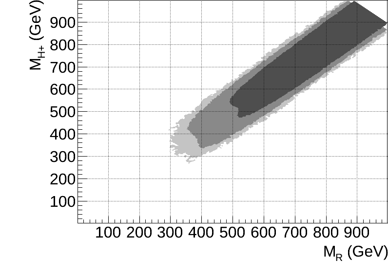
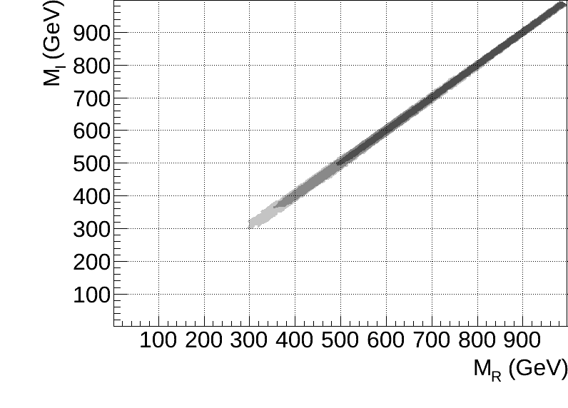
The main goal of this analysis is understanding which are the values of the new parameters – and masses of the scalars , and – allowed when all the previous constraints are imposed. This task is simplified by first paying attention to the effect of the precision electroweak constraints, in particular the oblique parameters. For similar values of , and , the oblique parameters are in good agreement with experimental data [16]. This fact is illustrated in figure 1, where the allowed regions corresponding to the usual 68%, 95% and 99% confidence levels are shown for a particular model, , after the constraints on the oblique parameters are imposed. Therefore, although all three masses are varied independently in the analyses, only results for one of them, , are displayed.
Figures 3 and 3, taken from [16], are the central result: they collect the allowed regions (68%, 95% and 99% confidence levels) in terms of and for all 36 models. Some comments are in order.
-
1.
Although tree level FCNC experimental constraints on down quark models are a priori tighter than on up quark models, up quark models are not less constrained due to the impact of on the allowed masses.
-
2.
Since and models give a stronger FCNC suppression – because of the hierarchical structure of the CKM matrix –, one would expect them to be less constrained; nevertheless, the effect of partially changes that picture and models are indeed less constrained than ones.
-
3.
It is important to stress that because of the strong suppression achieved for tree level FCNC, the importance of as a window to New Physics is enhanced, as the significant role played by shows.
-
4.
Notice however that, although provides relevant constraints, it is not as determinant as in type II 2HDM where it automatically forces GeV [19]; this is due to the different dependence in BGL models with respect to type II 2HDM (in addition, this dependence changes in the different BGL models).
-
5.
Concerning the leptonic part, since tree level neutrino FCNC are irrelevant (because of the small neutrino masses), , and are a priori less contrained than their neutrino counterparts, nevertheless such differences are insignificant: leptonic constraints are thus secondary once the effect of other constraints is considered.
-
6.
Lower bounds on the scalar masses are in the GeV ballpark for many models, opening the window to potential direct searches at the LHC. There are, however, some exceptions: models of types and require masses above GeV (although a wider range of values is acceptable in those models).
- 7.
5 Conclusions
Two Higgs doublet models of the Branco-Grimus-Lavoura class are a viable scenario where tree level Flavour Changing Neutral Currents arise in a controlled manner: they are proportional to mixings, fermion masses and . The present study shows that despite the existing tight experimental constraints, several types of BGL models are of immediate interest since they can accommodate new scalars light enough to be within direct experimental reach of the LHC.
Acknowledgments
MN thanks F.J. Botella, G.C. Branco, M.N. Rebelo and L. Pedro for constructive conversations and comments, and acknowledges financial support from Fundação para a Ciência e a Tecnologia (FCT, Portugal) through projects CFTP-FCT Unit 777 and CERN/FP/123580/2011, and MINECO (Spain) through grant FPA2011-23596.
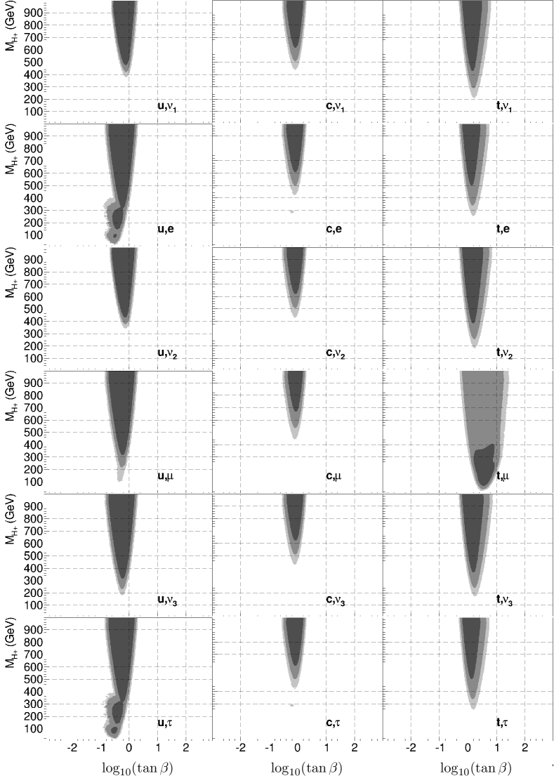
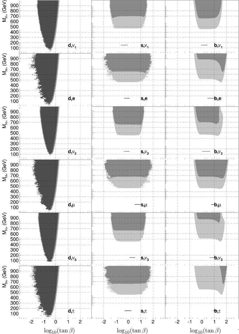
Summary plots of the allowed 68%, 95% and 99% CL regions in vs. for all BGL models.
References
- [1] G. Aad, et al., Observation of a new particle in the search for the Standard Model Higgs boson with the ATLAS detector at the LHC, Phys.Lett. B716 (2012) 1–29. arXiv:1207.7214, doi:10.1016/j.physletb.2012.08.020.
- [2] S. Chatrchyan, et al., Combined results of searches for the standard model Higgs boson in collisions at TeV, Phys.Lett. B710 (2012) 26–48. arXiv:1202.1488, doi:10.1016/j.physletb.2012.02.064.
- [3] T. Lee, A Theory of Spontaneous T Violation, Phys.Rev. D8 (1973) 1226–1239. doi:10.1103/PhysRevD.8.1226.
- [4] G. Branco, P. Ferreira, L. Lavoura, M. Rebelo, M. Sher, et al., Theory and phenomenology of two-Higgs-doublet models, Phys.Rept. 516 (2012) 1–102. arXiv:1106.0034, doi:10.1016/j.physrep.2012.02.002.
- [5] A. Crivellin, A. Kokulu, C. Greub, Flavor-phenomenology of two-Higgs-doublet models with generic Yukawa structure, Phys.Rev. D87 (9) (2013) 094031. arXiv:1303.5877, doi:10.1103/PhysRevD.87.094031.
- [6] S. L. Glashow, S. Weinberg, Natural Conservation Laws for Neutral Currents, Phys.Rev. D15 (1977) 1958. doi:10.1103/PhysRevD.15.1958.
- [7] E. Paschos, Diagonal Neutral Currents, Phys.Rev. D15 (1977) 1966. doi:10.1103/PhysRevD.15.1966.
- [8] A. Pich, P. Tuzon, Yukawa Alignment in the Two-Higgs-Doublet Model, Phys.Rev. D80 (2009) 091702. arXiv:0908.1554, doi:10.1103/PhysRevD.80.091702.
- [9] P. Ferreira, L. Lavoura, J. P. Silva, Renormalization-group constraints on Yukawa alignment in multi-Higgs-doublet models, Phys.Lett. B688 (2010) 341–344. arXiv:1001.2561, doi:10.1016/j.physletb.2010.04.033.
- [10] A. S. Joshipura, S. D. Rindani, Naturally suppressed flavor violations in two Higgs doublet models, Phys.Lett. B260 (1991) 149–153. doi:10.1016/0370-2693(91)90983-W.
- [11] L. Lavoura, Models of CP violation exclusively via neutral scalar exchange, Int.J.Mod.Phys. A9 (1994) 1873–1888. doi:10.1142/S0217751X94000807.
- [12] G. Branco, W. Grimus, L. Lavoura, Relating the scalar flavor changing neutral couplings to the CKM matrix, Phys.Lett. B380 (1996) 119–126. arXiv:hep-ph/9601383, doi:10.1016/0370-2693(96)00494-7.
- [13] F. Botella, G. Branco, M. Rebelo, Minimal Flavour Violation and Multi-Higgs Models, Phys.Lett. B687 (2010) 194–200. arXiv:0911.1753, doi:10.1016/j.physletb.2010.03.014.
- [14] F. Botella, G. Branco, M. Nebot, M. Rebelo, Two-Higgs Leptonic Minimal Flavour Violation, JHEP 1110 (2011) 037. arXiv:1102.0520, doi:10.1007/JHEP10(2011)037.
- [15] F. Botella, G. Branco, M. Rebelo, Invariants and Flavour in the General Two-Higgs Doublet Model, Phys.Lett. B722 (2013) 76–82. arXiv:1210.8163, doi:10.1016/j.physletb.2013.03.022.
- [16] F. Botella, G. Branco, A. Carmona, M. Nebot, L. Pedro, M. Rebelo, Physical Constraints on a Class of Two-Higgs Doublet Models with FCNC at tree level, JHEP 1407 (2014) 078. arXiv:1401.6147, doi:10.1007/JHEP07(2014)078.
- [17] G. Bhattacharyya, D. Das, A. Kundu, Feasibility of light scalars in a class of two-Higgs-doublet models and their decay signatures, Phys.Rev. D89 (2014) 095029. arXiv:1402.0364, doi:10.1103/PhysRevD.89.095029.
- [18] F. Botella, M. Nebot, O. Vives, Invariant approach to flavor-dependent CP-violating phases in the MSSM, JHEP 0601 (2006) 106. arXiv:hep-ph/0407349, doi:10.1088/1126-6708/2006/01/106.
- [19] T. Hermann, M. Misiak, M. Steinhauser, in the Two Higgs Doublet Model up to Next-to-Next-to-Leading Order in QCD, JHEP 1211 (2012) 036. arXiv:1208.2788, doi:10.1007/JHEP11(2012)036.
- [20] A. Buras, P. Gambino, M. Gorbahn, S. Jager, L. Silvestrini, Universal unitarity triangle and physics beyond the standard model, Phys.Lett. B500 (2001) 161–167. arXiv:hep-ph/0007085, doi:10.1016/S0370-2693(01)00061-2.
- [21] G. D’Ambrosio, G. Giudice, G. Isidori, A. Strumia, Minimal flavor violation: An Effective field theory approach, Nucl.Phys. B645 (2002) 155–187. arXiv:hep-ph/0207036, doi:10.1016/S0550-3213(02)00836-2.