Compression of the electron repulsion integral tensor in tensor hypercontraction format with cubic scaling cost

Abstract

Electron repulsion integral tensor has ubiquitous applications in electronic structure computations. In this work, we propose an algorithm which compresses the electron repulsion tensor into the tensor hypercontraction format with $\mathcal{O}(nN^{2}\log N)$ computational cost, where $N$ is the number of orbital functions and $n$ is the number of spatial grid points that the discretization of each orbital function has. The algorithm is based on a novel strategy of density fitting using a selection of a subset of spatial grid points to approximate the pair products of orbital functions on the whole domain.

I Introduction

Given a set of orbital functions $\{\psi_{i}\}\subset L^{2}(\mathbb{R}^{3})$, the four-center two-electron repulsion integrals

$$(ij|kl)=\iint_{\mathbb{R}^{3}\times\mathbb{R}^{3}}\frac{\psi_{i}(x)\psi_{j}(x)\psi_{k}(y)\psi_{l}(y)}{\lvert x-y\rvert}\,\mathrm{d}x\,\mathrm{d}y$$ (1)

are universally used in many electronic structure theories, such as Hartree-Fock, density functional theory (DFT), RPA, MP2, CCSD, and GW. As a result, a key step to accelerate ab initio computations in quantum chemistry and materials science is to get an efficient representation of the electron repulsion integral tensor.

One of the most popular methods for compressing the electron repulsion integral is the density fitting approximation. This method, also known as resolution of identity approach Ren et al. (2012); Dunlap et al. (1979); Schütz et al. (2010); Sodt et al. (2006); Vahtras et al. (1993); Weigend et al. (1998), amounts to representing pair products of orbital functions $\psi_{i}(x)\psi_{j}(x)$ in terms of a set of auxiliary basis functions

$$\rho_{ij}(x):=\psi_{i}(x)\psi_{j}(x)\approx\widetilde{\rho}_{ij}(x)=\sum_{\mu}C_{ij}^{\mu}P_{\mu}(x),$$ (2)

where $\mu=1,2,\ldots,N_{\mathrm{aux}}$ labels the auxiliary basis functions. The auxiliary basis functions are constructed either explicitly (e.g., a set of Gaussian-type atom-centered basis functions) or implicitly by using singular value decomposition on the overlap matrix of the set of $N^{2}$ functions $\rho_{ij}(x)$ Foerster (2008); Foerster et al. (2011).

After the auxiliary basis functions are determined, a least square fitting is used to determine the coefficient $C_{ij}^{\mu}$. When the standard $L^{2}$ metric is used in the least square fitting, one obtains

$$C_{ij}^{\mu}=\sum_{\nu}\langle ij|\nu\rangle S_{\nu\mu}^{-1},$$ (3)

$$(ij|kl)\approx\sum_{\mu\mu^{\prime}\nu\nu^{\prime}}\langle ij|\nu\rangle S_{\nu\mu}^{-1}V_{\mu\mu^{\prime}}S_{\mu^{\prime}\nu^{\prime}}^{-1}\langle\nu^{\prime}|kl\rangle$$ (4)

with the short-hand notations

$$\langle ij|\nu\rangle=\int\psi_{i}(x)\psi_{j}(x)P_{\nu}(x)\,\mathrm{d}x,$$ (5)

$$S_{\mu\nu}=\int P_{\mu}(x)P_{\nu}(x)\,\mathrm{d}x,\qquad\text{and}$$ (6)

$$V_{\mu\nu}=\iint\frac{P_{\mu}(x)P_{\nu}(y)}{\lvert x-y\rvert}\,\mathrm{d}x\,\mathrm{d}y.$$ (7)

It is also possible to use the Coulomb weight in the least square fitting, which leads to

$$C_{ij}^{\mu}=\sum_{\nu}(ij|\nu)V_{\nu\mu}^{-1},$$ (8)

$$(ij|kl)\approx\sum_{\mu\nu}(ij|\mu)V_{\mu\nu}^{-1}(\nu|kl)$$ (9)

with the short-hand notation

$$(ij|\nu)=\iint\frac{\psi_{i}(x)\psi_{j}(x)P_{\nu}(y)}{\lvert x-y\rvert}\,\mathrm{d}x\,\mathrm{d}y.$$ (10)

A closely related idea to density fitting is the incomplete Cholesky decomposition of the electron repulsion integrals Beebe and Linderberg (1977); Koch et al. (2003):

$$(ij|kl)\approx\sum_{\mu=1}^{M}L_{ij}^{\mu}L_{kl}^{\mu},$$ (11)

where $L_{ij}^{\mu}$ are numerically obtained Cholesky vectors. The cost of getting the resolution of identity approximation, assuming $\mathcal{O}(N)$ auxiliary basis functions, is $\mathcal{O}(N^{4})$, where $N$ is the number of orbital functions. Other methods for the electron repulsion integral tensor include multipole moment approaches Greengard and Rokhlin (1987); White et al. (1994, 1996); Strain et al. (1996) and pseudospectral representation Friesner (1985); Martinez et al. (1992); Martinez and Carter (1995).

More recently, the tensor hypercontraction of the electron repulsion integral have been proposed in Hohenstein et al. (2012); Parrish et al. (2012, 2013), which aims at an approximation of the electron repulsion integral tensor as

$$(ij|kl)\approx\sum_{\mu\nu}X_{i}^{\mu}X_{j}^{\mu}Z^{\mu\nu}X_{k}^{\nu}X_{l}^{\nu},$$ (12)

where $\mu,\nu$ are the indices for the decomposition. The factor $X$ is taken to be the weighted collocation matrix arises from numerical quadrature of the electron repulsion integral and $Z$ is determined by a least square procedure. The computational cost of obtaining the approximation is either $\mathcal{O}(N^{5})$ when direct quadrature of electron repulsion integral is used or $\mathcal{O}(N^{4})$ with the help of density fitting procedure. The tensor hypercontraction opens doors to efficient algorithms for several electronic structure theories, see e.g., Hohenstein et al. (2013, 2012); Parrish et al. (2012, 2014); Shenvi et al. (2013, 2014).

In this work, we propose an $\mathcal{O}(nN^{2}\log N)$ algorithm to get the tensor hypercontraction of the electron repulsion integral. It is based on an approximation of $\rho_{ij}(x)$ similar to (2), but with the key advantage that the coefficient $C_{ij}^{\mu}$ has separate dependence on the indices $i$ and $j$. Such an approximation is achieved by an interpolative decomposition which chooses selected grid points $x_{\mu}$ to interpolate the pair product density $\rho_{ij}$. This is different from the usual density fitting strategy with a predetermined set of auxiliary basis functions. In this sense, our algorithm tries to find an optimal set of the auxiliary basis functions, such that the tensor hypercontraction format can be immediately obtained.

II Algorithm

Our algorithm is based on the randomized column selection method for low-rank matrix, recently developed in Liberty et al. (2007); Woolfe et al. (2008). For an $m\times n$ matrix $A$, the column selection method looks for an interpolative decomposition to approximate $A\approx CP$ such that the discrepancy $\left\lVert A-CP\right\rVert$ is minimized, where $C$ is an $m\times c$ matrix consists of $c$ columns of $A$ and $P$ is a $c\times n$ matrix. The interpolative decomposition based on randomized column selection has recently been used for finding Wannier functions given a set of eigenfunctions in Kohn-Sham density functional theory Damle et al. (2014) by one of the authors. Here we demonstrate the power of the interpolative decomposition in the context of compressing electron repulsion integral tensor.

In our context, we will apply the column selection method on $\rho_{ij}(x)$ which is viewed as an $(N^{2})\times n$ matrix, where $N$ is the number of orbitals $\psi_{i}$ and $n$ is the total number of spatial grid points, i.e., we will view the pair $(ij)$ as the row index and the grid point $x$ as the column index of the matrix. We remark that while we will treat $x$ as a spatial grid throughout the presentation for definiteness, in other words, we have assumed a real space discretization of $\psi_{i}$, in fact, it is also possible to extend the algorithm to other discretizations, e.g., atomic orbitals, by using the idea proposed in pseudospectral representation Friesner (1985); Martinez et al. (1992); Martinez and Carter (1995). Let us emphasize that the choice of the spatial quadrature grid $x$ is completely general in our methods.

The column selection then amounts to choose a number of spatial grid points, denoted as $x_{\mu}$, $\mu=1,\ldots,N_{\mathrm{aux}}$, such that $\rho_{ij}(x)$ is approximated as

$$\rho_{ij}(x)\approx\sum_{\mu}\rho_{ij}(x_{\mu})P_{\mu}(x)=\sum_{\mu}\psi_{i}(x_{\mu})\psi_{j}(x_{\mu})P_{\mu}(x).$$ (13)

This should be compared with the approximation in the density fitting (2): Here $\psi_{i}(x_{\mu})\psi_{j}(x_{\mu})$ plays the role of the coefficient $C_{ij}^{\mu}$ in (2), which is the key feature of the interpolative decomposition approximation. To avoid possible confusion, unlike what is commonly involved in conventional density fitting approaches, the approximation (13) is not a quadrature formula, it should be understood as an interpolation. In particular, this should be distinguished from the flavor of tensor hypercontraction known as X-THC in Parrish et al. (2013), which is essentially a Gaussian quadrature formula for the overlap integrals.

The approximation (13) has a clear advantage that the dependence on $i$ and $j$ are separated as a result of using the selected columns to approximate the whole matrix. Indeed, assuming such an approximation (13), the electron repulsion integral tensor then becomes

$$(ij|kl)\approx\sum_{\mu\nu}\psi_{i}(x_{\mu})\psi_{j}(x_{\mu})V_{\mu\nu}\psi_{k}(x_{\nu})\psi_{j}(x_{\nu}).$$ (14)

Hence, we immediately arrive at the tensor hypercontraction format of the electron repulsion integral tensor without further approximation! The only extra step is to calculate $(\mu|\nu)$, which can be done efficiently using fast Fourier transform (FFT).

It remains to show how an approximation as (13) can be efficiently obtained. As opposed to the density fitting approach, the central focus in our algorithm is the selection of columns. After $N_{\mathrm{aux}}$ grid points $x_{\mu}$ are determined, the auxiliary basis functions $P_{\mu}$ follow from least squares fitting. To find the suitable subset of columns, a pivoted QR algorithm Golub and Van Loan (2013) is used on a random projection of $\rho_{ij}(x)$. In more details, the algorithm for the column selection consists of the following steps, given $\rho_{ij}(x)$ and an error threshold $\epsilon$.

1. Reshape $\rho_{ij}(x)$ into an $(N^{2})\times n$ matrix by combining $(ij)$ as a single index:

   $$\varrho_{(i-1)N+j}(x)=\rho_{ij}(x),$$ (15)

   where the index of $\varrho$, which will be denoted as $I$ in the following, goes from $1$ to $N^{2}$;

2. Random Fourier projection of $\varrho_{I}(x)$:

   1. Compute for $\xi=1,\ldots,N^{2}$ the discrete Fourier transform

      $$\mathfrak{M}_{\xi}(x)=\sum_{I=1}^{N^{2}}e^{-2\pi\sqrt{-1}I\xi/N^{2}}\eta_{I}\varrho_{I}(x),$$ (16)

      where $\eta_{I}$ is a random unit complex number for each $I$.

   2. Choose a submatrix $M$ of $N^{2}\times n$ matrix $\mathfrak{M}$ by randomly choosing $rN$ rows. In practice, $r=20$ is used in our implementation.

3. Compute the pivoted QR decomposition of the $rN\times n$ matrix $M$: $ME=QR$, where $E$ is an $n\times n$ permutation matrix, $Q$ is a $rN\times rN$ unitary matrix, and $R$ is a $rN\times n$ upper triangular matrix with diagonal entries in decreasing order.

   Note that $ME$ amounts to a permutation of the columns of $M$.

4. Determine the number of auxiliary basis functions $N_{\mathrm{aux}}$, such that $\lvert R_{N_{\mathrm{aux}}+1,N_{\mathrm{aux}}+1}\rvert<\epsilon\lvert R_{1,1}\rvert\leq\lvert R_{N_{\mathrm{aux}},N_{\mathrm{aux}}}\rvert$, i.e., this is a thresholding of the diagonals of $R$ to the relative error threshold $\epsilon$.

5. Choose $x_{\mu}$, $\mu=1,\ldots,N_{\mathrm{aux}}$ such that the $x_{\mu}$-column of $M$ corresponds to one of the first $N_{\mathrm{aux}}$ columns of $ME$.

6. Denote $R_{1:N_{\mathrm{aux}},1:N_{\mathrm{aux}}}$ the submatrix of $R$ consists of its first $N_{\mathrm{aux}}\times N_{\mathrm{aux}}$ entries, and $R_{1:N_{\mathrm{aux}},\boldsymbol{:}}$ the submatrix consists of the first $N_{\mathrm{aux}}$ rows of $R$. Compute

   $$P=R_{1:N_{\mathrm{aux}},1:N_{\mathrm{aux}}}^{-1}R_{1:N_{\mathrm{aux}},\boldsymbol{:}}\,E^{-1}.$$

   Then each row of the $N_{\mathrm{aux}}\times n$ matrix $P$ gives an auxiliary basis function $P_{\mu}(x)$ for $\mu=1,\ldots,N_{\mathrm{aux}}$.

The computationally expensive steps of the above algorithm are Steps 2, 3, and 6. Step 2 takes $n$ times FFT of $N^{2}$ length vectors, and hence has complexity $\mathcal{O}(nN^{2}\log N)$. Step 3 computes QR decomposition of $M$, which has complexity $\mathcal{O}(nN^{2})$. Step 6 involves inversion of an $N_{\mathrm{aux}}\times N_{\mathrm{aux}}$ matrix and multiply the inverse with an $N_{\mathrm{aux}}\times n$ matrix, which has complexity $\mathcal{O}(N_{\mathrm{aux}}^{3}+nN_{\mathrm{aux}}^{2})$. Hence, the overall complexity of the column selection is $\mathcal{O}(nN^{2}\log N)$, as $N_{\mathrm{aux}}=\mathcal{O}(N)$. The memory storage cost of the intermediate results is also $\mathcal{O}(nN^{2})$, which is the same as the cost of storing each entry of $\rho_{ij}(x)$.

Note that the Fourier transform in Step 2 of the algorithm acts on the index of the pair densities, but not the spatial grids. The Fourier transform is used for the random projection. We emphasize again that our algorithm does not rely on any particular choice of the spatial grids.

III Numerical results

Given a set of orbital functions $\{\psi_{i}\}$, we denote $\widetilde{\rho}_{ij}$ the result of the approximation based on the column selection method in the previous section. We measure the error in two ways by using the $L^{2}$ metric and the Coulomb metric:

$$e_{ij}^{(2)}=\biggl{(}\int\lvert\rho_{ij}(x)-\widetilde{\rho}_{ij}(x)\rvert^{2}\,\mathrm{d}x\biggr{)}^{2};$$ (17)

$$e_{ij}^{(c)}=\biggl{(}\iint\frac{(\rho_{ij}-\widetilde{\rho}_{ij})(x)(\rho_{ij}-\widetilde{\rho}_{ij})(y)}{\lvert x-y\rvert}\,\mathrm{d}x\,\mathrm{d}y\biggr{)}^{1/2}.$$ (18)

Note that the approximation error of the electron repulsion tensor can be controlled by $\max e_{ij}^{(c)}$, since we have

$$(ij|kl)-\sum_{\mu\nu}\psi_{i}(x_{\mu})\psi_{j}(x_{\mu})(\mu|\nu)\psi_{k}(x_{\nu})\psi_{l}(x_{\nu})$$ (19)

$$\quad=\iint\frac{\rho_{ij}(x)\rho_{kl}(y)-\widetilde{\rho}_{ij}(x)\widetilde{\rho}_{kl}(y)}{\lvert x-y\rvert}\,\mathrm{d}x\,\mathrm{d}y$$

$$\quad=\iint\frac{\rho_{ij}(x)(\rho_{kl}(y)-\widetilde{\rho}_{kl}(y))}{\lvert x-y\rvert}\,\mathrm{d}x\,\mathrm{d}y$$

$$\quad\qquad+\iint\frac{(\rho_{ij}(x)-\widetilde{\rho}_{ij}(x))\widetilde{\rho}_{kl}(y)}{\lvert x-y\rvert}\,\mathrm{d}x\,\mathrm{d}y$$

$$\quad\leq\left\lVert\rho_{ij}\right\rVert_{C}e_{kl}^{(c)}+e_{ij}^{(c)}\left\lVert\widetilde{\rho}_{kl}\right\rVert_{C},$$

where the last inequality follows from the Cauchy-Schwartz inequality and $\left\lVert\cdot\right\rVert_{C}$ stands for the Coulomb norm:

$$\left\lVert f\right\rVert_{C}=\biggl{(}\iint\frac{f(x)f(y)}{\lvert x-y\rvert}\,\mathrm{d}x\,\mathrm{d}y\biggr{)}^{1/2}.$$ (20)

We first test the performance of the algorithm for an $1D$ toy problem where the orbital functions are chosen to be the first $N$ eigenfunctions of a Hamiltonian operator $H=-\tfrac{1}{2}\Delta+V$, discretized on an interval rescaled to $[0,1]$ with $n=1024$ grid points, the periodic boundary conditions are used. To be consist with the periodic boundary condition, we replace the bare Coulomb interaction with the periodic Coulomb interaction to take into account the interaction with periodic images. Taking $V$ to be a potential randomly generated that consists of the first $128$ Fourier modes on $[0,1]$, we first diagonalize the discretized Hamiltonian to obtain $\{\psi_{i}\}$ and then apply the column selection method. We test the performance using different values of the threshold $\epsilon$ in Step 4 of the algorithm. The result is shown in Table 1, where the dimensionless relative errors are defined to be

$$\text{rel.~{}$2$-error}=\text{mean}(e_{ij}^{(2)})/\text{mean}\left\lVert\rho_{ij}\right\rVert_{2};$$ (21)

$$\text{rel.~{}c-error}=\text{mean}(e_{ij}^{(c)})/\text{mean}\left\lVert\rho_{ij}\right\rVert_{C},$$ (22)

where the average is taken with respect to the $N^{2}$ indices $(ij)$. We observe that the error measured in both the $L^{2}$ metric and the Coulomb metric is well controlled by the threshold $\epsilon$ with a small number of auxiliary functions. Note that we have $N^{2}=16384$ pair of orbitals in this example, while $10^{-5}$ relative error is achieved with $N_{\mathrm{aux}}$ around $300$. We also note that the number of auxiliary functions only increase mildly as we reduce the error threshold.

$\epsilon$	$N_{\mathrm{aux}}$	$\max e_{ij}^{(2)}$	$\max e_{ij}^{(c)}$	rel. $2$-error	rel. c-error
1E-5	300	1.477E-7	9.154E-6	6.806E-6	1.051E-5
1E-6	324	1.095E-8	8.626E-7	9.747E-7	1.366E-6
1E-7	353	1.877E-9	2.035E-7	1.086E-7	1.610E-7

Table 1: Error of the density fitting by column selection in $1D$ with $N=128$ and $n=1024$.

To test the computational complexity of the algorithm, we use a range of $N$ and $n$ while keeping the same error threshold $\epsilon=10^{-5}$. The timing results are shown in Table 2 together with the error of the fitting. The algorithm is implemented using Matlab and the test is done on a single core on Intel Xeon CPU X5690 3.47GHz. The timing matches very well with the complexity $\mathcal{O}(nN^{2}\log N)$. The linear dependence of $N_{\mathrm{aux}}$ on $N$ is also apparent.

$N$	$n$	$N_{\mathrm{aux}}$	rel. $2$-error	rel. c-error	time
64	512	154	7.101E-6	1.534E-5	0.077s
128	512	287	5.591E-6	3.472E-6	0.217s
128	1024	304	1.011E-5	2.707E-5	0.467s
256	1024	584	7.214E-6	6.268E-6	1.550s
256	2048	593	1.089E-5	2.555E-5	4.244s
512	2048	1156	5.355E-6	4.533E-6	17.881s

Table 2: Error and timing of the density fitting by column selection in $1D$ for fixed $\epsilon=10^{-5}$ and different $N$ and $n$.

To further test the algorithm in $3D$, we perform a $3D$ generalization of the numerical test in $1D$, where the orbital functions are taken to be collection of eigenfunctions of a given Hamiltonian operator. Here we take $n=4096$ degrees of freedom for each orbital $\psi_{i}$ and vary $N$ the number of orbital functions and $\epsilon$ the error threshold to evaluate the performance of the algorithm. The results are shown in Table 3. We observe that the relative error is still well controlled by the error threshold $\epsilon$, while in $3D$ we need more auxiliary basis functions compared to $1D$ case. For different $N$ and fixed error threshold $\epsilon$, the number of auxiliary basis functions grows roughly linearly with respect to $N$, confirming the scaling $N_{\mathrm{aux}}=\mathcal{O}(N)$. Note that in all cases, $N_{\mathrm{aux}}$ is much smaller compared with the total possible pair of orbitals $N^{2}$. The computational time also agrees well with $\mathcal{O}(nN^{2}\log N)$ (note that $n$ is fixed in this example).

$\epsilon$	$N$	$N_{\mathrm{aux}}$	$\max e_{ij}^{(c)}$	rel. $2$-error	rel. c-error	time
1E-4	32	303	1.863E-4	1.115E-4	6.290E-5	1.856s
1E-5	32	358	2.462E-5	1.676E-5	8.966E-6	1.892s
1E-6	32	407	3.429E-6	2.442E-6	1.280E-6	1.906s
1E-4	64	647	2.027E-4	1.126E-4	5.879E-5	6.403s
1E-5	64	767	2.257E-5	1.648E-5	8.330E-6	6.429s
1E-6	64	891	2.891E-6	2.484E-6	1.209E-6	6.431s
1E-4	128	1323	2.006E-4	1.018E-4	5.259E-5	20.046s
1E-5	128	1516	1.913E-5	1.285E-5	6.367E-6	20.212s
1E-6	128	1731	2.538E-6	1.661E-6	7.868E-7	20.497s

Table 3: Error and timing of the density fitting by column selection in $3D$ with $n=4096$.

Finally, we consider a more realistic example based on the implementation of the proposed algorithm in KSSOLV Yang et al. (2009), a MATLAB toolbox for solving the Kohn-Sham equations. For the test example, we choose two unit cells of a graphene sheet (and hence consisting of $4$ carbon atoms) with periodic boundary condition. Planewave is used for spatial discretization with a fixed energy cutoff, and hence $n$ is fixed. We take the first $N$ orbitals of the self-consistent Hamiltonian to be the collection of orbitals for density fitting. The error threshold $\epsilon$ is fixed for different $N$. The results are shown in Table 4. To compare the algorithm with conventional density fitting based on least square fitting with $L^{2}$ metric, we also include the timing of the conventional calculation of the coefficient based on the same auxiliary basis obtained in the proposed algorithm. The comparison of timing is further illustrated in Figure 1 (right). Since $n$ is fixed in this test, our algorithm scales as $N^{2}\log N$ and the conventional density fitting scales as $N^{3}$, which are clearly seen on the figure. Hence, for large $N$, the current algorithm has lower computational cost, even compared to density fitting, which is a preliminary step to get hypercontraction format. The Figure 1 (left) verifies the linear scaling dependence of $N_{\mathrm{aux}}$ on $N$. We note that except for a pre-asymptotic regime for small $N$, the linear dependence is clear.

$N$	$N_{\mathrm{aux}}$	rel. $2$-error	rel. c-error	time (proposed alg.)	time (least sq. fit)
8	36	5.658E-12	5.555e-12	1.148s	0.0161s
40	819	1.346E-4	6.571E-5	6.713s	1.130s
72	1968	6.803E-4	2.922e-4	15.310s	8.548s
104	2486	3.939E-4	1.770E-4	25.890s	21.239s
136	2877	2.360E-4	1.119E-4	36.607s	41.514s
168	3394	8.068E-5	3.796E-5	55.244s	75.074s
200	3782	4.685E-5	2.163E-5	73.514s	130.041s

Table 4: Error and timing of the density fitting by column selection (implemented in KSSOLV) for fixed $\epsilon=10^{-5}$, $n=10602$ and different $N$.

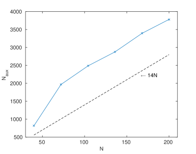
(a)

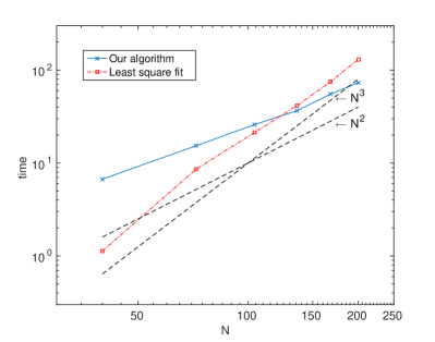
(b)

Figure 1: (left) $N_{\mathrm{aux}}$ as a function of $N$. The dash line provides a reference of the linear dependence on $N$. (right) Comparison of timing of the current algorithm and the conventional density fitting based on least square fitting. The dash lines provide reference of quadratic and cubic dependence on $N$.

IV Discussion and conclusion

The proposed cubic scaling algorithm for tensor hypercontraction format of electron repulsion integral tensor is easy to implement and can be easily incorporated into existing electronic structure packages. Relatively small scale numerical tests are done in this manuscript to demonstrate the effectiveness of the algorithm. Applications to large scale electronic structure calculations are the natural next steps.

The algorithm applies to general collection of orbital functions. In particular, we do not assume any locality of the functions $\{\psi_{i}\}$ in the algorithm. If a set of localized orbitals / basis functions are considered, it is then possible to utilize the locality to further reduce the computational cost. For instance, for a sub-collection of the orbitals, we may localize the column selection to the support of them. It would then even possible to reduce the computational scaling to $\mathcal{O}(N)$ with controllable error. This is an important future direction that we plan to pursue.

We also remark that for the simplicity of the presentation, here we have assumed that the orbital function $\psi_{i}$s are already represented on a real space grid. We emphasize that the choice of the spatial grid can be quite flexible. For example, if atomic orbital discretization is used, one can first get a real space representation using quadrature grids and then apply our algorithm. The computational complexity depends on $n$, the number of spatial grid points, which in practice will be a constant factor of $N$, while this prefactor might be large. It would be interesting to explore algorithms that can work directly with atomic orbital functions without first going to the real space representation.

Also related to the previous point of changing basis functions. The column selection method is designed with the discrepancy given by the Frobenius norm, i.e., $L^{2}$ metric. While our numerical tests have shown that the performance measured in error in either $L^{2}$ metric or Coulomb metric is satisfactory, one observes that the error in Coulomb metric is slightly larger than in the $L^{2}$ metric. It is therefore interesting to ask whether the column selection can be done in Coulomb metric directly. The natural idea of working on the Fourier domain does not work, as the Fourier transform in $x$ will destroy the separability of the dependence of the coefficients $C_{ij}^{\mu}$ on which the algorithm crucially depends on. To avoid possible confusion, let us emphasize that while the column selection uses $L^{2}$ metric, the density fitting proposed by the current algorithm is actually quite different from the RI-SVS density fitting (see e.g, the review article Ren et al. (2012)).

Finally, it would be interesting to explore fast algorithms for quantum chemistry calculations based on the $\mathcal{O}(nN^{2}\log N)$ algorithm for tensor hypercontraction proposed here.

Acknowledgment. J.L. would like to thank Weitao Yang for helpful discussions. The work of J.L. is supported in part by the Alfred P. Sloan Foundation and the National Science Foundation under grant DMS-1312659. The work of L.Y. is partially supported by the National Science Foundation under grant DMS-0846501 and the U.S. Department of Energy’s Advanced Scientific Computing Research program under grant DE-FC02-13ER26134/DE-SC0009409.

References

- Beebe and Linderberg [1977] N.H.F. Beebe and J. Linderberg. Simplifications in the generation and transformation of two-electron integrals in molecular calculations. Int. J. Quantum Chem., 12:683–705, 1977. URL http://dx.doi.org/10.1002/qua.560120408.
- Damle et al. [2014] A. Damle, L. Lin, and L. Ying. Compressed representation of Kohn-Sham orbitals via selected columns of the density matrix, 2014. URL http://www.arxiv.org/abs/1408.4926/. preprint, arXiv:1408.4926.
- Dunlap et al. [1979] B. I. Dunlap, J. W. D. Connolly, and J. R. Sabin. On first-row diatomic molecules and local density models. J. Chem. Phys., 71:4993–4999, 1979. URL http:/dx.doi.org/10.1063/1.438313.
- Foerster [2008] D. Foerster. Elimination, in electronic structure calculations, of redundant orbital products. J. Chem. Phys., 128:034108, 2008. URL http://dx.doi.org/10.1063/1.2821021.
- Foerster et al. [2011] D. Foerster, P. Koval, and D. Sánchez-Portal. An implementation of Hedin’s GW approximation for molecules. J. Chem. Phys., 135:074105, 2011. URL http://dx.doi.org/10.1063/1.3624731.
- Friesner [1985] R. A. Friesner. Solution of self-consistent field electronic structure equations by a pseudospectral method. Chem. Phys. Lett., 116:39–43, 1985. URL http://dx.doi.org/10.1016/0009-2614(85)80121-4.
- Golub and Van Loan [2013] G.H. Golub and C.F. Van Loan. Matrix computations. Johns Hopkins Studies in the Mathematical Sciences. Johns Hopkins University Press, Baltimore, MD, fourth edition, 2013.
- Greengard and Rokhlin [1987] L. Greengard and V. Rokhlin. A fast algorithm for particle simulations. J. Comput. Phys., 73:325–348, 1987. URL http://dx.doi.org/10.1016/0021-9991(87)90140-9.
- Hohenstein et al. [2013] E. G. Hohenstein, S. I. L. Kokkila, R. M. Parrish, and T. J. Martinez. Quartic scaling second-order approximate coupled cluster singles and doubles via tensor hypercontraction: THC-CC2. J. Chem. Phys., 138:124111, 2013. URL http://dx.doi.org/10.1063/1.4795514.
- Hohenstein et al. [2012] E.G. Hohenstein, R.M. Parrish, and T.J. Martinez. Tensor hypercontraction density fitting. I. Quartic scaling second- and third-order Møller-plesset perturbation theory. J. Chem. Phys., 137:044103, 2012. URL http://dx.doi.org/10.1063/1.4732310.
- Koch et al. [2003] H. Koch, A. Sánchez de Merás, and T. B. Pedersen. Reduced scaling in electronic structure calculations using Cholesky decompositions. J. Chem. Phys., 118:9481–9484, 2003. URL http://dx.doi.org/10.1063/1.1578621.
- Liberty et al. [2007] E. Liberty, F. Woolfe, P.-G. Martinsson, V. Rokhlin, and M. Tygert. Randomized algorithms for the low-rank approximation of matrices. Proc. Natl. Acad. Sci. USA, 104:20167–20172, 2007. URL http://dx.doi.org/10.1073/pnas.0709640104.
- Martinez and Carter [1995] T. J. Martinez and E. A. Carter. Pseudospectral methods applied to the electron correlation problem. In D. R. Yarkony, editor, Modern Electronic Structure Theorry Part II, volume 2 of Advanced Series in Physical Chemistry, pages 1132–1165. World Scientific, Singapore, 1995.
- Martinez et al. [1992] T. J. Martinez, A. Mehta, and E. A. Carter. Pseudospectral full configuration interaction. J. Chem. Phys., 97:1876 – 1880, 1992. URL http://dx.doi.org/10.1063/1.463176.
- Parrish et al. [2013] R. M. Parrish, E. G. Hohenstein, N. F. Schunck, C. D. Sherrill, and T. J. Martinez. Exact tensor hypercontraction: A universal technique for the resolution of matrix elements of local finite-range N-body potentials in many-body quantum problems. Phys. Rev. Lett., 111:132505, 2013. URL http://dx.doi.org/10.1103/PhysRevLett.111.132505.
- Parrish et al. [2014] R. M. Parrish, C. David Sherrill, E. G. Hohenstein, S. I. L. Kokkila, and T. J. Martinez. Communication: Acceleration of coupled cluster singles and doubles via orbital-weighted least-squares tensor hypercontraction. J. Chem. Phys., 140:181102, 2014. URL http://dx.doi.org/10.1063/1.4876016.
- Parrish et al. [2012] R.M. Parrish, E.G. Hohenstein, T.J. Martinez, and C. David Sherrill. Tensor hypercontraction. II. Least-squares renormalization. J. Chem. Phys., 137:224106, 2012. URL http://dx.doi.org/10.1063/1.4768233.
- Ren et al. [2012] X. Ren, P. Rinke, V. Blum, J. Wieferink, A. Tkatchenko, A. Sanfilippo, K. Reuter, and M. Scheffler. Resolution-of-identity approach to Hartree-Fock, hybrid density functionals, RPA, MP2 and GW with numeric atom-centered orbital basis functions. New J. Phys., 14:053020, 2012. URL http://dx.doi.org/10.1088/1367-2630/14/5/053020.
- Schütz et al. [2010] M. Schütz, D. Usvyat, M. Lorenz, C. Pisani, L. Maschio, S. Casassa, and M. Halo. Density fitting for correlated calculations in periodic systems. In F. Manby, editor, Accurate Condensed-Phase Quantum Chemistry, Computation in Chemistry, page 27. CRC Press, 2010. URL http://dx.doi.org/10.1201/9781439808375-c2.
- Shenvi et al. [2013] N. Shenvi, H. van Aggelen, Y. Yang, W. Yang, C. Schwerdtfeger, and D. Mazziotti. The tensor hypercontracted parametric reduced density matrix algorithm: Coupled-cluster accuracy with scaling. J. Chem. Phys., 139:054110, 2013. URL http://dx.doi.org/10.1063/1.4817184.
- Shenvi et al. [2014] N. Shenvi, H. van Aggelen, Y. Yang, and W. Yang. Tensor hypercontracted ppRPA: Reducing the cost of the particle-particle random phase approximation from to . J. Chem. Phys., 141:024119, 2014. URL http://dx.doi.org/10.1063/1.4886584.
- Sodt et al. [2006] A. Sodt, J. E. Subotnik, and M. Head-Gordon. Linear scaling density fitting. J. Chem. Phys., 125:194109, 2006. URL http://dx.doi.org/10.1063/1.2370949.
- Strain et al. [1996] M. C. Strain, G. E. Scuseria, and M. J. Frisch. Achieving linear scaling for the electronic quantum Coulomb problem. Science, 271:51–53, 1996. URL http://dx.doi.org/10.1126/science.271.5245.51.
- Vahtras et al. [1993] O. Vahtras, J. Almlöf, and M. W. Feyereisen. Integral approximations for LCAO-SCF calculations. Chem. Phys. Lett., 213(5–6):514–518, 1993. URL http://dx.doi.org/10.1016/0029-2614(93)89151-7.
- Weigend et al. [1998] F. Weigend, M. Häser, H. Patzelt, and R. Ahlrichs. RI-MP2: optimized auxiliary basis sets and demonstration of efficiency. Chem. Phys. Lett., 294(1–3):143–152, 1998. URL http://dx.doi.org/10.1016/S0009-2614(98)00862-8.
- White et al. [1994] C. A. White, B. G. Johnson, P.M.W. Gill, and M. Head-Gordon. The continuous fast multipole method. Chem. Phys. Lett., 230:8–16, 1994. URL http://dx.doi.org/10.1016/0009-2614(94)01128-1.
- White et al. [1996] C. A. White, B. G. Johnson, P.M.W. Gill, and M. Head-Gordon. Lienar scaling density functional calculations via the continuous fast multipole method. Chem. Phys. Lett., 253:268–278, 1996. URL http://dx.doi.org/10.1016/0009-2614(96)00175-3.
- Woolfe et al. [2008] F. Woolfe, E. Liberty, V. Rokhlin, and M. Tygert. A fast randomized algorithm for the approximation of matrices. Appl. Comput. Harmon. Anal., 25:335 – 366, 2008. URL http://dx.doi.org/10.1016/j.acha.2007.12.002.
- Yang et al. [2009] C. Yang, J. C. Meza, B. Lee, and L.-W. Wang. KSSOLV–a MATLAB toolbox for solving the Kohn-Sham equations. ACM T. Math. Software, 36(2):10, 2009.