Almost Sure Asymptotic Stability for Regime-Switching Diffusions

Abstract

In this paper, we discuss long-time behavior of sample paths for a wide range of regime-switching diffusions. Firstly, almost sure asymptotic stability is concerned (i) for regime-switching diffusions with finite state spaces by the Perron-Frobenius theorem, and, with regard to the case of reversible Markov chain, via the principal eigenvalue approach; (ii) for regime-switching diffusions with countable state spaces by means of a finite partition trick and an M-Matrix theory. We then apply our theory to study the stabilization for linear switching models. Several examples are given to demonstrate our theory.

AMS subject Classification: 60H10; 93D15
Keywords: almost sure asymptotic stability, averaging condition, Perron-Frobenius’s theorem, principal eigenvalue, M-matrix,

1 Introduction

Stochastic stability of stochastic differential equations (SDEs) has been well developed (see e.g. the monographs [7, 10, 14]. For a regime-switching diffusion, we mean a diffusion process in a random environment characterized by a Markov chain. Its state vector is a pair $(X_{t},\Lambda_{t})$, where the continuous component $X_{t}$ is referred to as the state, while the discrete component $\Lambda_{t}$ is regarded as the mode. Regime-switching diffusions have been widely applied in control problems, storage modeling, neutral activity, biology and mathematical finance (see e.g. [13, 26]). In particular, an important issue in the study of regime-switching diffusions is concerned with stability. In the past three decades, stochastic stability of regime switching diffusions has also received great attention (see e.g. the monographs [13, 26]). [13, Exampe 5.45, p.223] reveals that $X_{t}$ is stable although some of the subsystems are not. So, in most cases, stability analysis for regime-switching processes may be markedly differently different from that of SDEs with regime switching. So far, the work on stability analysis for regime-switching processes focus on moment exponential stability [8, 11, 12], almost sure exponent stability [15, 22], asymptotically stable in probability [8, 19, 26], stability in distribution [23, 24], to name a few. For ergodic property, strong Feller, transience and recurrence for regime-switching diffusions, we would like to refer to [2, 16, 17, 18, 19, 21] and references therein.

For most existing results, condition to guarantee stability are irrespective of stationary distribution of Markov chain involved (see e.g. [11, 12, 15, 22, 23, 24, 26]). Moreover, note that the vast majority of stability analysis focus on regime-switching diffusions with finite state spaces (see e.g. [11, 12, 15, 22, 23, 24, 26]). In this paper, under some new conditions (see Theorems 3.1, 3.4 and 5.1 for more details), we shall discuss stability analysis of sample paths for a class of regime-switching diffusions which may admit infinite state spaces. The content of this paper is arranged as follows. In Section 3, for regime-switching diffusions with finite state spaces, under an “averaging condition”we study almost sure asymptotic stability of sample path (see Theorem 3.1) by the Perron-Frobenius theorem. In particular, Theorem 3.1 improves greatly some existing results (see e.g. [27, Theorem 3.1] and [13, Theorem 5.29, p.192]). For more details, please refer to Examples 3.6 and 3.7. Section 4 is devoted to diffusion processes with reversible Markov chains. For such special case, the principal eigenvalue approach is adopted to deal with almost sure asymptotic stability (see Theorem 3.4), where Theorem 3.4 cannot be covered by Theorem 3.1 as Example 4.2 shows. Note that Theorem 3.1 is dependent on the explicit formula of stationary distribution of Markov chain, and Theorem 4.1 need the principal eigenvalue to be attainable. Accordingly, Theorems 3.1 and 3.4 seem hard to be generalized to the counterpart with infinite state space. Nevertheless, for a regime-switching diffusion with an infinite state space, in Section 5, by a finite partition trick and an M-matrix theory, we proceed to investigate almost sure asymptotic stability.

2 Problem Setup

For each integer $n>0$, let $(\mathbb{R}^{n},\langle\cdot,\cdot\rangle,|\cdot|)$ be the $n$-dimensional Euclidean space and $\mathbb{R}^{n}\otimes\mathbb{R}^{m}$ the totality of all $n\times m$ matrices endowed with the Frobenius norm $\|\cdot\|$. Let $\{W_{t}\}_{t\geq 0}$ be an $m$-dimensional Brownian motion defined on the probability space $(\Omega,\mathscr{F},\mathbb{P})$ with a filtration $\{\mathscr{F}_{t}\}_{t\geq 0}$ satisfying the usual conditions (i.e., $\mathscr{F}_{t}=\mathscr{F}_{t+}:=\bigcap_{s>t}\mathscr{F}_{s}$ and $\mathscr{F}_{0}$ contains all $\mathbb{P}$-null sets). If $A$ is a vector or matrix, its transpose is denoted by $A^{T}$. Let ${\bf 0}$ be a zero vector, for $\xi=(\xi_{1},\cdots,\xi_{n})^{T}\in\mathbb{R}^{n}$, $\xi\gg{\bf 0}(\mbox{resp. }\xi\ll{\bf 0})$ means each component $\xi_{i}>0(\mbox{resp. }\xi_{i}<0)$, $i=1,\cdots,n.$ $C^{2}(\mathbb{R}^{n};\mathbb{R}_{+})$ stands for the family of all nonnegative functions $f:\mathbb{R}^{n}\times\mathbb{R}_{+}\mapsto\mathbb{R}_{+}$ which are continuously twice differentiable.

In this paper, we focus on a regime-switching diffusion process $(X_{t},\Lambda_{t})$, where $\{X_{t}\}_{t\geq 0}$ satisfies an SDE on $(\mathbb{R}^{n},\langle\cdot,\cdot\rangle,|\cdot|)$

$$\text{\rm{d}}X_{t}=b(X_{t},t,\Lambda_{t})\text{\rm{d}}t+\sigma(X_{t},t,\Lambda_{t})\text{\rm{d}}W_{t},~{}t>0,~{}X_{0}=x_{0},~{}\Lambda_{0}=i_{0},$$ (2.1)

and $\{\Lambda_{t}\}_{t\geq 0}$, independent of the Brownian motion $\{W_{t}\}_{t\geq 0}$, is a right-continuous Markov chain defined on the probability space $(\Omega,\mathscr{F},\mathbb{P})$ with the state space $\mathbb{S}:=\{1,2,\cdots,N\}$ for some $1\leq N\leq\infty$ and the transition rules specified by

$$\mathbb{P}(\Lambda_{t+\delta}=j|\Lambda_{t}=i)=\begin{cases}q_{ij}\delta+o(\delta),~{}~{}~{}~{}~{}~{}~{}~{}i\neq j,\\ 1+q_{ii}\delta+o(\delta),~{}~{}~{}i=j\end{cases}$$ (2.2)

for sufficiently small $\delta>0$. Here $q_{ij}\geq 0$ is the transition rate from $i$ to $j$ if $i\neq j$ while $q_{ii}=-\sum_{i\neq j}q_{ij}.$ We assume that the $Q$-matrix $Q:=(q_{ij})_{N\times N}$ is irreducible so that the Markov chain $\{\Lambda_{t}\}_{t\geq 0}$ has a unique stationary distribution $\mu:=({\mu_{1},\cdots,\mu_{N}})$ which can be determined by solving the following linear equation

$$\mu Q={\bf 0}$$

subject to $\mu_{1}+\cdots+\mu_{N}=1~{}\mbox{ and }~{}\mu_{i}>0,\,i\in\mathbb{S}.$

It is well known that a continuous-time Markov chain $\{\Lambda_{t}\}_{t\geq 0}$ with generator $Q=(q_{ij})_{N\times N}$ can be described in the following manner by using the Poisson random measure. Let

$$h(i,z)=\sum_{j\in\mathbb{S}\setminus i}(j-i){\bf 1}_{z\in\triangle_{ij}},$$

where $\triangle_{ij}$ are the consecutive (with respect to (w.r.t.) the lexicographic order on $\mathbb{S}\times\mathbb{S}$ left-closed, right-open intervals on $\mathbb{R}_{+}$, each having length $q_{ij}$, with $\triangle_{12}=[0,q_{12})).$ Then

$$\text{\rm{d}}\Lambda_{t}=\int_{\mathbb{R}}h(X_{t-},z)N(\text{\rm{d}}t,\text{\rm{d}}z),~{}~{}~{}\Lambda_{0}=i_{0},$$

where $N(\text{\rm{d}}t,\text{\rm{d}}z)$ is a Poisson random measure with intensity $\text{\rm{d}}t\times\text{\rm{d}}z.$

Let $(X_{t},\Lambda_{t})$ be the regime-switching diffusion process determined by (2.1) and (2.2). For each fixed environment $i\in\mathbb{S}$, the corresponding diffusion $X_{t}^{(i)}$ is defined by

$$\text{\rm{d}}X_{t}^{(i)}=b(X_{t}^{(i)},t,i)\text{\rm{d}}t+\sigma(X_{t}^{(i)},t,i)\text{\rm{d}}W_{t},~{}~{}~{}t>0,~{}~{}~{}X_{0}^{(i)}=x_{0}.$$ (2.3)

Then, the infinitesimal generator associated with (2.3) is given by

$$\mathscr{L}^{(i)}_{t}V(x):=\langle\nabla V(x),b(x,t,i)\rangle+\frac{1}{2}\mbox{trace}(\sigma^{T}(x,t,i)\nabla^{2}V(x)\sigma(x,t,i)),~{}V\in C^{2}(\mathbb{R}^{n};\mathbb{R}_{+}),$$

where $\nabla$ and $\nabla^{2}$ stand for the gradient and Hessian operators respectively.

Throughout the paper, we assume that

1. $b:\mathbb{R}^{n}\times\mathbb{R}_{+}\times\mathbb{S}\mapsto\mathbb{R}^{n}$ and $\sigma:\mathbb{R}^{n}\times\mathbb{R}_{+}\times\mathbb{S}\mapsto\mathbb{R}^{n}\otimes\mathbb{R}^{m}$ satisfy the local Lipschitz condition with respect to (w.r.t.) the first variable, i.e., for each $k>0$, there exists an $L_{k}>0$ such that

   $$|b(x,t,i)-b(y,t,i)|+\|\sigma(x,t,i)-\sigma(y,t,i)\|\leq L_{k}|x-y|,~{}~{}~{}|x|\vee|y|\leq k,$$

   for all $(t,i)\in\mathbb{R}_{+}\times\mathbb{S}$. Moreover,

   $$\sup_{t\geq 0,i\in\mathbb{S}}\{|b(0,t,i)|+\|\sigma(0,t,i)\|\}<\infty.$$

2. For each fixed $i\in\mathbb{S}$, there exists a function $V\in C^{2}(\mathbb{R}^{n};\mathbb{R}_{+})$ and $\beta_{i}\in\mathbb{R}$ such that $\lim_{|x|\rightarrow\infty}V(x)=\infty,V(0)=0$ and

   $$\mathscr{L}^{(i)}_{t}V(x)\leq\beta_{i}V(x),~{}~{}~{}(x,t)\in\mathbb{R}^{n}\times\mathbb{R}_{+}.$$ (2.4)

Under (H1) and (H2), by the classical Khasminskii approach (see e.g. [7, Theorem 3.5, p.75]), (2.1) admits a unique strong solution $\{X_{t}(x_{0},i_{0})\}_{t\geq 0}$ to highlight the initial data $X_{0}=x_{0}$ and $\Lambda_{0}=i_{0}$.

Definition 2.1.

The solution of (2.1) is said to be almost surely asymptotically stable if, for all $x_{0}\in\mathbb{R}^{n}$ and $i_{0}\in\mathbb{S}$,

$$\mathbb{P}\left(\lim_{t\rightarrow\infty}|X_{t}(x_{0},i_{0})|=0\right)=1.$$

The lemma (see e.g. [9, Thorem 7, p.139])) below, which is concerned with long-time behavior of nonnegative semi-martingales, plays a crucial role in the following stability analysis of sample path for (2.1).

Lemma 2.1.

Let $\{A_{1}(t)\}_{t\geq 0}$, $\{A_{2}(t)\}_{t\geq 0}$ be two continuous adapted increasing processes with $A_{1}(0)=A_{2}(0)=0$ a.s., $M(t)$ a real-valued continuous local martingale with $M(0)=0$ a.s., and $\zeta$ a nonnegative $\mathscr{F}_{0}$-measurable random variable such that $\mathbb{E}\zeta<\infty$. Define

$$X(t)=\zeta+A_{1}(t)-A_{2}(t)+M(t),~{}~{}~{}t\geq 0.$$

If $X(t)$ is nonnegative, then

$$\left\{\lim_{t\rightarrow\infty}A_{1}(t)<\infty\right\}\subset\left\{\lim_{t\rightarrow\infty}X(t)<\infty\right\}\bigcap\left\{\lim_{t\rightarrow\infty}A_{2}(t)<\infty\right\}~{}~{}\mbox{a.s.},$$

where $C\subset D$ a.s. means $\mathbb{P}(C\cap D^{c})=0$. In particular, if $\lim_{t\rightarrow\infty}A_{1}(t)<\infty$ a.s., then,

$$\lim_{t\rightarrow\infty}X(t)<\infty,~{}~{}\lim_{t\rightarrow\infty}A_{2}(t)<\infty,~{}~{}\mbox{ and }~{}~{}-\infty<\lim_{t\rightarrow\infty}M(t)<\infty,~{}~{}~{}\mbox{a.s.}$$

3 Almost Sure Asymptotic Stability

Our main result in this section is stated as below. Throughout this section, we assume that the Markov state space is finite, i.e. $N<\infty.$

Theorem 3.1.

Let assumptions (H1) and (H2) hold. Suppose further that

$$\sum_{i=1}^{N}\mu_{i}\beta_{i}<0.$$ (3.1)

Then, the solution of (2.1) is almost surely asymptotically stable.

Remark 3.1.

Equation (2.1) is said to be attractive “in average” if (3.1) holds (see e.g. [2]). We call (3.1) an “averaging condition”. On the other hand, in Theorem 3.1, it is worth to pointing out that, for each $i\in\mathbb{S}$, $\beta_{i}$ need not to be negative.

Before the proof of Theorem 3.1, let us recall Proposition 4.2 due to Bardet et al. [2], which is stated as below for convenience.

Lemma 3.2.

For any $p>0$, let

$$\mbox{diag}(\beta):=\mbox{diag}(\beta_{1},\cdots,\beta_{N}),~{}~{}~{}~{}Q_{p}:=Q+p\,\mbox{diag}(\beta),~{}~{}\eta_{p}:=-\max_{\gamma\in\mbox{spec}(Q_{p})}\mbox{Re}\gamma,$$ (3.2)

where $Q$ is the $Q$-matrix of the Markov chain $\{\Lambda(t)\}_{t\geq 0},$ and $\mbox{spec}(Q_{p})$ denotes the spectrum of $Q_{p}.$ Under (3.1), one has

1. $\eta_{p}>0$ if $\max_{i\in\mathbb{S}}\beta_{i}\leq 0;$

2. $\eta_{p}>0$ for $p<\alpha$, where $\alpha\in(0,\min_{\beta_{i}>0,i\in\mathbb{S}}\{-q_{ii}/\beta_{i}\})$ with $\max_{i\in\mathbb{S}}\beta_{i}>0.$

We are now in the position to complete the argument of Theorem 3.1.

Proof of Theorem 3.1. Let $Q_{p,t}:=\text{\rm{e}}^{tQ_{p}}$, where $Q_{p}$ is defined as in (3.2). Then the spectral radius $\mbox{Ria}(Q_{p,t})$ of $Q_{p,t}$ equals to $\text{\rm{e}}^{-\eta_{p}}$. Since all coefficients of $Q_{p,t}$ are positive, the Perron-Frobenius theorem (see e.g. [6, p.6]) yields that $-\eta_{p}$ is a simple eigenvalue of $Q_{p}.$ Moreover, note that the eigenvalue of $Q_{p,t}$ corresponding to $\text{\rm{e}}^{-\eta_{p}}$ is also an eigenvalue of $Q_{p}$ corresponding to $-\eta_{p}.$ The Perron-Frobenius theorem (see e.g. [6, p.6]) ensures that there exists an eigenvector $\xi^{(p)}=(\xi_{1}^{(p)},\cdots,\xi_{N}^{(p)})\gg{\bf 0}$ of $Q_{p}$ corresponding to $-\eta_{p}.$ Now, by Lemma 3.2 above, there exists some $p_{0}>0$ such that $\eta_{p}>0$ for any $0<p<p_{0}.$ In what follows, fix a $p$ with $0<p\leq\min\{1,p_{0}\}$ and the corresponding eigenvector $\xi^{(p)}\gg{\bf 0}$. Then we obtain that

$$Q_{p}\xi^{(p)}=-\eta_{p}\xi^{(p)}\ll{\bf 0}.$$ (3.3)

For notation simplicity, in what follows, we write $\{X_{t}\}_{t\geq 0}$ in lieu of $\{X_{t}(x_{0},i_{0})\}_{t\geq 0}$. By the Itô formula, it follows that

$$\begin{split}V^{p}(X_{t})\xi^{(p)}_{\Lambda_{t}}&=V^{p}(x_{0})\xi^{(p)}_{i_{0}}+\int_{0}^{t}\{(\mathscr{L}^{(\Lambda_{s})}_{s}V^{p}(X_{s}))\xi^{(p)}_{\Lambda_{s}}+V^{p}(X_{s})(Q\xi^{(p)})(\Lambda_{s})\}\text{\rm{d}}s\\ &\quad+\int_{0}^{t}\xi^{(p)}_{\Lambda_{s}}\langle\nabla V^{p}(X_{s}),\sigma(X_{s},s,\Lambda_{s})\text{\rm{d}}W_{s}\rangle\\ &\quad+\int_{0}^{t}\int_{\mathbb{R}}V^{p}(X_{s})\{\xi^{(p)}_{i_{0}+h(\Lambda_{s},z)}-\xi^{(p)}_{\Lambda_{s}}\}\widetilde{N}(\text{\rm{d}}s,\text{\rm{d}}z)\\ &=:J_{1}(t)+J_{2}(t)+J_{3}(t)+J_{4}(t),\end{split}$$

where $(Q\xi^{(p)})(i),i\in\mathbb{S}$, denotes the $i$-th entry of the vector $Q\xi^{(p)}$, and $\widetilde{N}(\text{\rm{d}}t,\text{\rm{d}}z):=N(\text{\rm{d}}t,\text{\rm{d}}z)-\text{\rm{d}}t\text{\rm{d}}z$. Due to $p\in(0,1]$, observe from (2.4) and (3.1) that

$$\begin{split}J_{2}(t)&=\int_{0}^{t}\Big{\{}pV^{p-1}(X_{s})(\mathscr{L}^{(\Lambda_{s})}_{s}V(X_{s}))\xi^{(p)}_{\Lambda_{s}}+V^{p}(X_{s})(Q\xi^{(p)})(\Lambda_{s})\\ &\quad+\frac{p(p-1)}{2}V^{p-2}(X_{s})|\sigma^{T}(X_{s},s,\Lambda_{s})\nabla V(X_{s})|^{2}\Big{\}}\text{\rm{d}}s\\ &\leq\int_{0}^{t}\{p\beta_{\Lambda_{s}}\xi^{(p)}_{\Lambda_{s}}+(Q\xi^{(p)})(\Lambda_{s})\}V^{p}(X_{s})\text{\rm{d}}s\\ &=\int_{0}^{t}(Q_{p}\xi^{(p)})(\Lambda_{s})V^{p}(X_{s})\text{\rm{d}}s\\ &=-\eta_{p}\int_{0}^{t}\xi^{(p)}_{\Lambda_{s}}V^{p}(X_{s})\text{\rm{d}}s.\end{split}$$

Hence, we arrive at

$$\begin{split}V^{p}(X_{t})\xi^{(p)}_{\Lambda_{t}}&\leq V^{p}(x_{0})\xi^{(p)}_{i_{0}}-\eta_{p}\int_{0}^{t}\xi^{(p)}_{\Lambda_{s}}V^{p}(X_{s})\text{\rm{d}}s+J_{3}(t)+J_{4}(t).\end{split}$$

Note that $J_{3}(t)$ and $J_{4}(t)$ are local martingales. Set

$$Y(t):=V^{p}(x)\xi^{(p)}_{i_{0}}-\eta_{p}\int_{0}^{t}\xi^{(p)}_{\Lambda_{s}}V^{p}(X_{s})\text{\rm{d}}s+J_{3}(t)+J_{4}(t).$$

It is easy to see that $V^{p}(X_{t})\xi^{(p)}_{\Lambda_{t}}\leq Y(t)$, $\mbox{a.s.},$ and $Y(t)$ is a nonnegative semi-martingale. Thus, by Lemma 2.1, we infer that

$$\lim_{t\rightarrow\infty}V(X_{t})<\infty~{}~{}\mbox{a.s.}~{}~{}~{}~{}\mbox{ and }~{}~{}~{}~{}\int_{0}^{\infty}V^{p}(X_{t})\text{\rm{d}}t<\infty~{}~{}\mbox{a.s.}$$ (3.4)

This, together with $\lim_{|x|\rightarrow\infty}V(x)=\infty,$ further yields that

$$\sup_{0\leq t<\infty}|X_{t}|<\infty~{}~{}~{}\mbox{a.s.},$$

and,

$$\liminf_{t\rightarrow\infty}V(X_{t})=0~{}~{}\mbox{a.s.}.$$

Moreover, we can also claim that there exists $\Omega_{0}\subset\Omega$ with $\mathbb{P}(\Omega_{0})=1$ such that

$$\lim_{t\rightarrow\infty}V(X_{t}(\omega))=0,~{}~{}~{}\omega\in\Omega_{0}.$$ (3.5)

Then, by a contraction argument, we derive that

$$\lim_{t\rightarrow\infty}X_{t}(\omega)=0,~{}~{}~{}\omega\in\Omega_{0}.$$ (3.6)

The desired assertion is therefore complete. For more details on argument of (3.5) and (3.6), please refer to Appendix A.

In (H2), taking $V(x)=|x|^{2}$, we derive the following corollary.

Corollary 3.3.

Let (H1) hold. Assume that, for each $i\in\mathbb{S}$, there exists $\beta_{i}\in\mathbb{R}$ such that

$$2\langle x,b(x,t,i)\rangle+\|\sigma(x,t,i)\|^{2}\leq\beta_{i}|x|^{2},~{}~{}~{}\forall(x,t)\in\mathbb{R}^{n}\times\mathbb{R}_{+}.$$

Assume further that

$$\sum_{i=1}^{N}\mu_{i}\beta_{i}<0.$$

Then, the solution of (2.1) is almost surely asymptotically stable.

We assume that

1. For each $i\in\mathbb{S}$, there exist $V\in C^{2}(\mathbb{R}^{n};\mathbb{R}_{+})$ with compact level sets, $\gamma\in L^{1}(\mathbb{R}_{+};\mathbb{R}_{+})$, and $\beta_{i}\in\mathbb{R}$ such that

   $$\mathscr{L}^{(i)}_{t}V(x)\leq\gamma_{t}+\beta_{i}V(x),~{}~{}~{}(x,t)\in\mathbb{R}^{n}\times\mathbb{R}_{+}.$$ (3.7)

Theorem 3.4.

Let (H1) and (H$2^{\prime}$) hold. Assume further that

$$\min_{i\in\mathbb{S}}\{-q_{ii}/\beta_{i}:\beta_{i}>0\}>1,$$ (3.8)

and

$$\sum_{i=1}^{N}\mu_{i}\beta_{i}<0.$$ (3.9)

Then, the solution of (2.1) is almost surely asymptotically stable.

Proof.

Let

$$Q_{1}:=Q+\mbox{diag}(\beta_{1},\cdots,\beta_{N}),$$

where $\beta_{i}\in\mathbb{R}$ such that (3.9). Due to (3.8), upon following an argument of (3.3), there exist $\eta>0$ and a vector $\xi=(\xi_{1},\ldots,\xi_{N})\gg{\bf 0}$ such that

$$Q_{1}\xi=-\eta\xi\ll{\bf 0}.$$ (3.10)

By Itô’s formula, we derive from (3.7) and (3.10) that

$$\begin{split}V(X_{t})\xi_{\Lambda_{t}}&=V(x_{0})\xi_{i_{0}}+\int_{0}^{t}\{(\mathscr{L}_{s}^{(\Lambda_{s})}V(X_{s}))\xi_{\Lambda_{s}}+V(X_{s})(Q\xi)(\Lambda_{s})\}\text{\rm{d}}s+\Lambda_{1}(t)+\Lambda_{2}(t)\\ &\leq V(x_{0})\xi_{i_{0}}+\int_{0}^{t}\{\gamma_{s}\xi_{\Lambda_{s}}+(\beta_{\Lambda_{s}}\xi_{\Lambda_{s}}+(Q\xi)(\Lambda_{s}))V(X_{s})\}\text{\rm{d}}s+\Lambda_{1}(t)+\Lambda_{2}(t)\\ &=V(x_{0})\xi_{i_{0}}+\int_{0}^{t}\{\gamma_{s}\xi_{\Lambda_{s}}+(Q_{1}\xi)(\Lambda_{s})V(X_{s})\}\text{\rm{d}}s+\Lambda_{1}(t)+\Lambda_{2}(t)\\ &\leq V(x_{0})\xi_{i_{0}}+\max_{i\in\mathbb{S}}\xi_{i}\int_{0}^{t}\gamma_{s}\text{\rm{d}}s-\eta\int_{0}^{t}V(X_{s})\xi_{\Lambda_{s}}\text{\rm{d}}s+\Lambda_{1}(t)+\Lambda_{2}(t),\end{split}$$

where

$$\Lambda_{1}(t):=\int_{0}^{t}\xi_{\Lambda_{s}}\langle\nabla V(X_{t}),\sigma(X_{s},s,\Lambda_{s})\text{\rm{d}}W_{s}\rangle,~{}~{}\Lambda_{2}(t):=\int_{0}^{t}\int_{\mathbb{R}}V(X_{s})\{\xi_{i_{0}+h(\Lambda_{s},z)}-\xi_{\Lambda_{s}}\}\widetilde{N}(\text{\rm{d}}s,\text{\rm{d}}z).$$

Note that $\gamma\in L^{1}(\mathbb{R}_{+};\mathbb{R}_{+})$. Thus, the desired assertion follows by carrying out an argument of Theorem 3.1. ∎

In (H2’), taking $V(x)=|x|^{2}$, we deduce the corollary below.

Corollary 3.5.

Let (H1) hold. Assume that, for each $i\in\mathbb{S}$, there exists $\gamma\in L^{1}(\mathbb{R}_{+};\mathbb{R}_{+})$, and $\beta_{i}\in\mathbb{R}$ such that

$$2\langle x,b(x,t,i)\rangle+\|\sigma(x,t,i)\|^{2}\leq\gamma_{t}+\beta_{i}|x|^{2},~{}~{}~{}\forall(x,t)\in\mathbb{R}^{n}\times\mathbb{R}_{+}.$$

Assume further that

$$\sum_{i=1}^{N}\mu_{i}\beta_{i}<0.$$

Then, the solution of (2.1) is almost surely asymptotically stable.

In the sequel, we provide two examples to demonstrate applications of our theory.

Example 3.6.

Let $\{W_{t}\}_{t\geq 0}$ be a scalar Brownian motion. Consider a regime-switching diffusion process $(X_{t},\Lambda_{t})$, where $\{X_{t}\}_{t\geq 0}$ obeys a scalar SDE

$$\text{\rm{d}}X_{t}=b_{\Lambda_{t}}X_{t}\text{\rm{d}}t+\sigma_{\Lambda_{t}}X_{t}\text{\rm{d}}W_{t},$$ (3.11)

with initial value $(X_{0},\Lambda_{0}),$ and $\{\Lambda_{t}\}_{t\geq 0}$, independent of $\{W_{t}\}_{t\geq 0}$, is a right-continuous Markovian chain taking values in $\mathbb{S}=\{1,2\}$ with generator

$$Q=\left(\begin{array}[]{cc}-u&u\\ v&-v\\ \end{array}\right)$$

for $u,v>0$.

In (3.11), set $b_{1}=1,b_{2}=-2,\sigma_{1}=1,\sigma_{2}=1$. Note that the solution of SDE

$$\text{\rm{d}}X_{t}=X_{t}\text{\rm{d}}t+X_{t}\text{\rm{d}}W(t),~{}~{}t>0,~{}~{}~{}X_{0}=x_{0}$$

is unstable. It is easy to see that the unique stationary distribution of $\{\Lambda_{t}\}_{t\geq 0}$ is $(\mu_{1},\mu_{2})=(\frac{v}{u+v},\frac{u}{u+v})$. A straightforward calculation gives that

$$\mathscr{L}_{t}^{(1)}(|x|^{2})=3|x|^{2}~{}~{}~{}\mbox{ and }~{}~{}~{}\mathscr{L}_{t}^{(2)}(|x|^{2})=-3|x|^{2},~{}~{}~{}~{}x\in\mathbb{R}.$$

So $\beta_{1}=3,\beta_{2}=-3$. Thus, by Corollary 3.5, the solution of (3.11) is almost surely asymptotically stable if $0<v<u.$

However, in order for the solution of (3.11) is almost surely asymptotically stable, the condition in [27, Theorem 3.1] is $u>6$ and $v\in(0,3)$. Therefore, the present Theorem 3.1 improves some existing results in certain sense.

Example 3.7.

Let $\{W_{t}\}$ be a scalar Brownian motion. Consider a regime-switching diffusion process $(X_{t},\Lambda_{t})$, in which $\{X_{t}\}_{t\geq 0}$ satisfies a scalar SDE

$$\text{\rm{d}}X_{t}=b(X_{t},t,\Lambda_{t})\text{\rm{d}}t+\sigma(X_{t},t,\Lambda_{t})\text{\rm{d}}W(t),$$ (3.12)

with initial value $(X_{0},\Lambda_{0}),$ and $\{\Lambda_{t}\}_{t\geq 0}$, independent of $\{W_{t}\}_{t\geq 0}$, is a right-continuous Markovian chain taking values in $\mathbb{S}:=\{0,1,2\}$ with the generator

$$Q=\left(\begin{array}[]{ccc}-(3+\nu)&\nu&3\\ 1&-3&2\\ 1&2&-3\end{array}\right)$$ (3.13)

for some $\nu\geq 0.$ In (3.12), for any $(x,t)\in\mathbb{R}\times\mathbb{R}_{+},$ let

$$b(x,t,0)=\frac{x}{4},~{}~{}~{}~{}~{}~{}~{}~{}~{}~{}~{}~{}~{}~{}~{}~{}~{}~{}~{}~{}~{}~{}~{}~{}~{}~{}\sigma(x,t,0)=(1+t)^{-1},$$

$$b(x,t,1)=\sin x/(1+t),~{}~{}~{}~{}~{}~{}~{}~{}~{}~{}~{}~{}\sigma(x,t,1)=\frac{x}{2},$$

$$b(x,t,2)=\text{\rm{e}}^{-t}-5x-2x^{3},~{}~{}~{}~{}~{}~{}~{}~{}~{}\sigma(x,t,2)=x\sin t.$$

Note that the unique stationary distribution of $\{\Lambda_{t}\}_{t\geq 0}$ is

$$\mu=(\mu_{0},\mu_{1},\mu_{2})=\Big{(}\frac{5}{20+5\nu},\frac{6+3\nu}{20+5\nu},\frac{9+2\nu}{20+5\nu}\Big{)}.$$

Next, by the fundamental inequality: $2ab\leq\varepsilon a^{2}+b^{2}/\varepsilon$ for $a,b\in\mathbb{R},\varepsilon>0$, it follows that

$$\begin{split}\mathscr{L}^{(0)}_{t}(|x|^{2})=\frac{1}{(1+t)^{2}}+\frac{|x|^{2}}{2},~{}\mathscr{L}^{(1)}_{t}(|x|^{2})\leq\frac{4}{(1+t)^{2}}+\frac{|x|^{2}}{2},\end{split}$$

and

$$\begin{split}\mathscr{L}_{t}^{(2)}(|x|^{2})\leq\text{\rm{e}}^{-2t}-8|x|^{2}.\end{split}$$

Hence, $\beta_{0}=\beta_{1}=\frac{1}{2}$, $\beta_{2}=-8$, and $\gamma_{t}=4(1+t)^{-2}+\text{\rm{e}}^{-2t}$. For (3.12), it is trivial to see that (3.8) and (3.9) hold respectively. By Theorem 3.4, the solution of Eq.(3.12) is almost surely asymptotically stable.

Whereas, observe that $b(0,t,2)=\text{\rm{e}}^{-t}\neq 0$ and $b(x,t,2)$ don’t satisfy the linear growth condition so that [13, Theorem 5.29, p.192] does not apply to (3.12).

4 Almost Sure Asymptotic Stability: Reversible Case

In the last section, we investigate almost sure asymptotic stability for the regime-switching diffusion process determined by (2.1) and (2.3), where the Markov chain $\{\Lambda_{t}\}_{t\geq 0}$ need not to be reversible, i.e., $\pi_{i}q_{ij}=\pi_{j}q_{ji},i,j\in\mathbb{S}$, for some probability measure $\pi:=(\pi_{1},\cdots,\pi_{N})$. While, if $\{\Lambda_{t}\}_{t\geq 0}$ with finite state space, i.e., $N<\infty$, is reversible, under another new condition the long-time behavior of sample path for (2.1) can also be discussed as Theorem 4.1 below shows.

To begin with, we need to introduce some notation. Throughout this section, we always assume that $N<\infty$. Let

$$L^{2}(\pi):=\Big{\{}f\in\mathscr{B}(\mathbb{S}):\sum_{i=1}^{N}\pi_{i}f_{i}^{2}<\infty\Big{\}}.$$

Then $(L^{2}(\pi),\langle\cdot,\cdot\rangle_{0},\|\cdot\|_{0})$ is a Hilbert space with the inner product $\langle f,g\rangle_{0}:=\sum_{i=1}^{N}\pi_{i}f_{i}g_{i},f,g\in L^{2}(\pi)$. Define the bilinear form $(D(f),\mathscr{D}(D))$ as

$$D(f):=\frac{1}{2}\sum_{i,j=1}^{N}\pi_{i}q_{ij}(f_{j}-f_{i})^{2}-\sum_{i=1}^{N}\pi_{i}\beta_{i}f_{i}^{2},~{}~{}~{}f\in L^{2}(\pi),$$

where $\beta_{i}\in\mathbb{R},i\in\mathbb{S}$, is given in (H$2^{\prime}$), and the domain

$$\mathscr{D}(D):=\{f\in L^{2}(\pi):D(f)<\infty\}.$$

The principal eigenvalue $\lambda_{0}$ of $D(f)$ is defined by

$$\lambda_{0}:=\inf\{D(f):f\in\mathscr{D}(D),\|f\|_{0}=1\}.$$

For more details on the first eigenvalue, refer to [5, Chapter 3]. Due to the fact that the state space of $\{\Lambda_{t}\}_{t\geq 0}$ is finite, there exists $\xi=(\xi_{1},\cdots,\xi_{N})\in\mathscr{D}(D)$ such that

$$D(\xi)=\lambda_{0}\|\xi\|^{2}_{0}.$$ (4.1)

Define the operator

$$\overline{\Omega}:=Q+\mbox{diag}(\beta_{1},\cdots,\beta_{N}),$$

where $Q$ is the $Q$-matrix of $\{\Lambda_{t}\}_{t\geq 0},$ and $\beta_{i}\in\mathbb{R}$ such that (H$2^{\prime}$).

The main result in this section is the following.

Theorem 4.1.

Let (H1) and (H$2^{\prime}$) hold, and assume further $\lambda_{0}>0$. Then, the solution of (2.1) is almost surely asymptotically stable.

Proof.

Recalling (4.1) and checking the argument of [16, Theorem 3.2], one has

$$\xi\gg{\bf 0}~{}~{}\mbox{ and }~{}~{}(Q\xi)(i)+\beta_{i}\xi_{i}=-\lambda_{0}\xi_{i},~{}i\in\mathbb{S}.$$

Then, we complete the proof by carrying out an argument of Theorem 3.1. ∎

Next, an example is constructed to show Theorem 4.1.

Example 4.2.

Let $\{W_{t}\}$ be a scalar Brownian motion. Consider a regime-switching diffusion process $(X_{t},\Lambda_{t})$, in which $\{X_{t}\}_{t\geq 0}$ satisfies a scalar SDE

$$\text{\rm{d}}X_{t}=b(X_{t},t,\Lambda_{t})\text{\rm{d}}t+\sigma(X_{t},t,\Lambda_{t})\text{\rm{d}}W(t),~{}~{}X_{0}=x_{0},~{}~{}\Lambda_{0}=0,$$ (4.2)

and $\{\Lambda_{t}\}_{t\geq 0}$, independent of $\{W_{t}\}_{t\geq 0}$, is a right-continuous Markovian chain taking values in $\mathbb{S}:=\{0,1,2\}$

$$Q=\left(\begin{array}[]{ccc}-b&b&0\\ 2a&-2(a+b)&2b\\ 0&3a&-3a\end{array}\right)$$

for $a,b>0$ such that

$$b\in(0,1/4)~{}~{}~{}~{}\mbox{ and }~{}~{}~{}~{}a-b>1.$$ (4.3)

In (4.2), for any $(x,t)\in\mathbb{R}\times\mathbb{R}_{+},$ let

$$b(x,t,0)=-x/8,~{}~{}~{}~{}~{}~{}~{}~{}~{}~{}~{}~{}~{}~{}~{}~{}~{}~{}~{}~{}~{}\sigma(x,t,0)=(1+t)^{-1},$$

$$b(x,t,1)=\sin x/(1+t),~{}~{}~{}~{}~{}~{}~{}~{}~{}~{}~{}~{}\sigma(x,t,1)=x,$$

$$b(x,t,2)=\text{\rm{e}}^{-t}-x/6-2x^{3},~{}~{}~{}~{}~{}~{}~{}\sigma(x,t,2)=(x\sin t)/2.$$

Hence, one can take $\beta_{0}=-1/4,\beta_{1}=1+\varepsilon$, $\beta_{2}=-1/3+\delta$ for sufficiently small $\varepsilon,\delta>0$, and $\gamma_{t}=c_{\varepsilon,\delta}((1+t)^{-2}+\text{\rm{e}}^{-2t})$ for some $c_{\varepsilon,\delta}>0$. Moreover, by the notion of $\Omega$, for $\xi_{i}=i+1$, $i=0,1,2,$ we deduce that

$$\begin{split}(\overline{\Omega}\xi)(0)=-(-b-\beta_{0})\xi_{0},~{}~{}(\overline{\Omega}\xi)(1)=-(a-b-\beta_{1})\xi_{1},~{}~{}(\overline{\Omega}\xi)(2)=-(a-\beta_{2})\xi_{2}.\end{split}$$

Due to (4.3), we can chose $\varepsilon,\delta>0$ sufficiently small such that

$$\lambda=\min\{-b-\beta_{0},a-b-\beta_{1},a-\beta_{2}\}>0.$$

Thus, one finds that

$$(\overline{\Omega}\xi)(i)\leq-\lambda\xi_{i},~{}~{}~{}i=0,1,2.$$

Then $\lambda_{0}>0$ due to [16, Theorem 4.4]. As a result, by Theorem 3.4, the solution of (4.2) is almost surely asymptotically stable.

Note that the unique stationary distribution of $\{\Lambda_{t}\}_{t\geq 0}$ is $\mu=(1/3,1/3,1/3),$ and it is easy to see that the averaging condition (3.9) does not hold no matter how small $\varepsilon,\delta>0$ is. Hence Corrolary 3.5 does not apply to (3.9). Consequently, Theorem 4.1 has its own right.

5 Almost Sure Asymptotic Stability: Countable State Space

For the case of finite state space (i.e. $N<\infty$), we adopt the Perron-Frobenius theorem and the principal eigenvalue approach to study almost sure asymptotic stability for regime-switching diffusion process determined by (2.1) and (2.2), respectively. With regard to the first method, the averaging condition (see (3.1)) plays an important role in the stability analysis. Therefore, one has to provide an explicit formula of stationary distribution for an irreducible Markov chain to guarantee the averaging condition to hold under some appropriate conditions. So this approach seems hard to be generalized to the case of infinite state space (i.e. $N=\infty$) since the explicit expression of stationary distribution is hard to be obtained. On the other hand, the principal eigenvalue approach can also be extend to the case of infinite state space, however, under an additional condition that $\lambda_{0}$ is attainable, i.e., there exists $f\in L^{2}(\pi),f\neq 0$, such that $D(f)=\lambda_{0}\|f\|_{0}^{2}.$ In this section, for the case of infinite state space, by a finite partition approach and an $M$-matrix theory, we proceed to discuss almost sure asymptotic stability for regime-switching diffusion process determined by (2.1) and (2.2).

Definition 5.1.

(see e.g. [13, Definition 2.9, p.67]) A square matrix $A=(a_{ij})_{n\times n}$ is called a nonsingular $M$-matrix if $A$ can be expressed in the form $A=sI-B$ with $B\gg{\bf 0}$ and $s>\mbox{Ria}(B)$, where $I$ is the $n\times n$ identity matrix and $\mbox{Ria}(B)$ the spectral radius of $B.$

We further suppose that

$$K:=\sup_{i\in\mathbb{S}}\beta_{i}<\infty~{}~{}~{}~{}\mbox{ and }~{}~{}~{}~{}\sup_{i\in\mathbb{S}}(-q_{ii})<\infty.$$ (5.1)

Let us insert $m$ points in the interval $(-\infty,K]$ as follows:

$$-\infty=:k_{0}<k_{1}<\cdots<k_{m}<k_{m+1}:=K.$$

Then, the interval $(-\infty,K]$ is divided into $m+1$ sub-intervals $(k_{i-1},k_{i}]$ indexed by $i$. Let

$$F_{i}:=\{j\in\mathbb{S}:\beta_{j}\in(k_{i-1},k_{i}]\},~{}~{}i=1,\cdots,m+1.$$

Without loss of generality, we can and do assume that each $F_{i}$ is not empty. Then

$$F:=\{F_{1},\cdots,F_{m+1}\}$$

is a finite partition of $\mathbb{S}$. For $i,j=1,\cdots,m+1$, set

$$q_{ij}^{F}:=\begin{cases}\sup_{r\in F_{i}}\sum_{k\in F_{j}}q_{rk},~{}~{}~{}~{}~{}~{}~{}~{}j<i,\\ \inf_{r\in F_{i}}\sum_{k\in F_{j}}q_{rk},~{}~{}~{}~{}~{}~{}~{}~{}~{}j>i,\\ -\sum_{j\neq i}q_{ij}^{F},~{}~{}~{}~{}~{}~{}~{}~{}~{}~{}~{}~{}~{}~{}~{}~{}~{}i=j.\end{cases}$$

So $Q^{F}:=(q_{ij}^{F})$ is the $Q$-matrix for some Markov chain with the state space $\mathbb{S}_{0}:=\{1,\cdots,m+1\}.$ For $i=1,\cdots,m+1$, let

$$\beta_{i}^{F}:=\sup_{j\in F_{i}}\beta_{j},~{}~{}~{}~{}~{}~{}~{}~{}H_{m+1}:=\left(\begin{array}[]{ccccc}1&1&1&\cdots&1\\ 0&1&1&\cdots&1\\ \vdots&\vdots&\vdots&\cdots&\vdots\\ 0&0&0&\cdots&1\\ \end{array}\right)_{(m+1)\times(m+1)}.$$

Theorem 5.1.

Let $N=\infty$, and assume that (H1), (H$2^{\prime}$) and (5.1) hold. Assume further that

$$-(Q^{F}+\mbox{diag}(\beta_{1}^{F},\cdots,\beta_{m+1}^{F}))H_{m+1}$$

is a nonsingular $M$-matrix. Then, the solution of (2.1) is almost surely asymptotically stable.

Proof.

Since $-(Q^{F}+\mbox{diag}(\beta_{1}^{F},\cdots,\beta_{m+1}^{F}))H_{m+1}$ is a nonsingular $M$-matrix, by [13, Theorem 2.10, p.68] there exists a vector $\eta^{F}:=(\eta_{1}^{F},\cdots,\eta_{m+1}^{F})^{*}\gg{\bf 0}$ such that

$$(-\lambda_{1}^{F},\cdots,-\lambda_{m+1}^{F})^{*}:=(Q^{F}+\mbox{diag}(\beta_{1}^{F},\cdots,\beta_{m+1}^{F}))H_{m+1}\eta^{F}\ll{\bf 0}.$$ (5.2)

Set $\xi^{F}:=H_{m+1}\eta^{F}$. By the structure of $H_{m+1}$, it is trivial to see that

$$\xi_{i}^{F}=\eta^{F}_{m+1}+\cdots+\eta^{F}_{i},~{}~{}i=1,\cdots,m+1.$$

This, together with $\eta^{F}\gg{\bf 0}$, yields that $\xi^{F}\gg{\bf 0}$ and $\xi^{F}_{i+1}<\xi^{F}_{i},i=1,\cdots,m+1$. Next, we extend the vector $\xi^{F}$ to be a vector on $\mathbb{S}$ by setting $\xi_{r}:=\xi_{i}^{F}$ for $r\in F_{i}$. Moreover, let $\phi:\mathbb{S}\mapsto\{1,\cdots,m+1\}$ be a map defined by $\phi(j):=i$ for $j\in F_{i}.$ Then, by the definition of $\beta_{i}^{F}$, one has

$$\xi_{r}=\xi_{i}^{F}=\xi_{\phi(r)}^{F}~{}\mbox{ and }~{}\beta_{r}\leq\beta^{F}_{\phi(r)},~{}~{}~{}r\in F_{i}.$$ (5.3)

For any $r\in\mathbb{S}$, there exists $F_{i}$ such that $r\in F_{i}$. Recalling the definition of $q_{ij}^{F}$ and utilizing $\xi^{F}_{i+1}<\xi^{F}_{i},i=1,\cdots,m+1$, we derive from (5.3) that, for $r\in F_{i}$,

$$\begin{split}(Q\xi)(r)&=\sum_{k<i}\sum_{j\in F_{k}}q_{rj}(\xi_{j}-\xi_{r})+\sum_{k>i}\sum_{j\in F_{k}}q_{rj}(\xi_{j}-\xi_{r})\\ &=\sum_{k<i}\sum_{j\in F_{k}}q_{rj}(\xi_{k}^{F}-\xi_{i}^{F})+\sum_{k>i}\sum_{j\in F_{k}}q_{rj}(\xi_{k}^{F}-\xi_{i}^{F})\\ &\leq\sum_{k<i}q_{ik}^{F}(\xi_{k}^{F}-\xi_{i}^{F})+\sum_{k>i}q_{ik}^{F}(\xi_{k}^{F}-\xi_{i}^{F})\\ &=(Q^{F}\xi^{F})(i)=(Q^{F}\xi^{F})(\phi(r)).\end{split}$$ (5.4)

Observe from (5.2)-(5.4) that

$$\begin{split}&V(X_{t})\xi_{\Lambda_{t}}\\ &\leq V(x_{0})\xi_{i_{0}}+\int_{0}^{t}\{\gamma_{s}\xi_{\Lambda_{s}}+((Q\xi)(\Lambda_{s})+\beta_{\Lambda_{s}}\xi_{\Lambda_{s}})V(X_{s})\}\text{\rm{d}}s+\Gamma_{1}(t)+\Gamma_{2}(t)\\ &\leq V(x_{0})\xi_{i_{0}}+\int_{0}^{t}\{\gamma_{s}\xi_{\phi(\Lambda_{s})}^{F}+((Q^{F}\xi^{F})(\phi(\Lambda_{s}))+\beta^{F}_{\phi(\Lambda_{s})}\xi_{\phi(\Lambda_{s})}^{F})V(X_{s})\}\text{\rm{d}}s+\Gamma_{1}(t)+\Gamma_{2}(t)\\ &\leq|x_{0}|^{2}\xi_{i_{0}}+\mu\int_{0}^{t}\gamma_{s}\text{\rm{d}}s-\nu\int_{0}^{t}V(X_{s})\text{\rm{d}}s+\Gamma_{1}(t)+\Gamma_{2}(t),\end{split}$$

where $\mu:=\max_{i\in\mathbb{S}_{0}}\lambda_{i}^{F}$, $\nu:=\min_{i\in\mathbb{S}_{0}}\lambda_{i}^{F}$ due to (5.2), and

$$\Gamma_{1}(t):=2\int_{0}^{t}\xi_{\phi(\Lambda_{s})}^{F}\langle\nabla V(X_{s}),\sigma(X_{s},s,\Lambda_{s})\text{\rm{d}}W_{s}\rangle,~{}\Gamma_{2}(t):=\int_{0}^{t}\int_{\mathbb{R}}V(X_{s})\{\xi_{\phi(i_{0}+h(\Lambda_{s},z))}^{F}-\xi_{\phi(\Lambda_{s})}^{F}\}\widetilde{N}(\text{\rm{d}}s,\text{\rm{d}}z).$$

Then, the desired assertion follows by imitating an argument of Theorem 3.1. ∎

Before the end of this paper, an example is established to demonstrate Theorem 4.1.

Example 5.2.

Let $\{X_{t}\}_{t\geq 0}$ satisfy a scalar SDE

$$\text{\rm{d}}X_{t}=b_{\Lambda_{t}}X_{t}\text{\rm{d}}t+X_{t}^{2}\wedge|X_{t}|\text{\rm{d}}W_{t},~{}~{}~{}X_{0}=x_{0}\neq 0$$ (5.5)

and $\{\Lambda_{t}\}_{t\geq 0}$ is a birth-death process on $\mathbb{S}:=\{1,2,\cdots\}$ with $q_{ii+1}=c_{i}>0,$ $q_{ii-1}=a_{i}>0$, and $q_{ij}=0$ for $|i-j|>1$. Let $b_{1}=-1,b_{i}=\kappa-i^{-1},i\geq 2,$ for some $\kappa>0,$ and assume $\sup_{i\in\mathbb{S}}(-q_{ii})<\infty$ with $q_{ii}=-(a_{i}+c_{i})$. Note that

$$\mathscr{L}_{t}^{(i)}(|x|)=b_{i}|x|,~{}~{}~{}i\in\mathbb{S}.$$

Thus (5.1) holds for $\beta_{i}=b_{i}$, and $\beta_{1}^{F}=-1,\beta_{2}^{F}=\kappa$. Set $F_{1}=\{1\}$ and $F_{2}=\{2,3,\cdots\}$. Due to $q_{ij}=0$ for $|i-j|>1$. Then we have

$$-Q^{F}=\left(\begin{array}[]{cc}-c_{1}&c_{1}\\ a_{2}&-a_{2}\\ \end{array}\right).$$

As a consequence, if $\kappa\in(0,a_{2}/(1+c_{1})),$ the solution of (5.5) is almost surely asymptotically stable since $-(Q^{F}+\mbox{diag}(\beta_{1}^{F},\beta_{2}^{F}))H_{2}$ is a nonsingular $M$-matrix. While, under the same condition, Shao and Xi [19, Example 2.1] shows that the solution of (5.5) is asymptotically stable in probability.

6 Stabilization of linear regime-switching diffusions

Let us now consider the following linear regime-switching diffusions:

$$\text{\rm{d}}X_{t}=A_{\Lambda_{t}}X_{t}\text{\rm{d}}t+\sum^{m}_{k=1}C^{(k)}_{\Lambda_{t}}X_{t}\text{\rm{d}}W^{(k)}_{t},$$ (6.1)

on$t\geq 0$ with initial data $x(0)=x_{0}\in\mathbb{R}^{n}$ and $\Lambda_{0}=i_{0}\in\mathbb{S}$.

We are required to design a state feedback control $u_{t}$ in the drift part such that the corresponding controlled system

$$\text{\rm{d}}X_{t}=[A_{\Lambda_{t}}X_{t}+B_{\Lambda_{t}}u_{t}]\text{\rm{d}}t+\sum^{m}_{k=1}C^{(k)}_{\Lambda_{t}}X_{t}\text{\rm{d}}W^{(k)}_{t},$$ (6.2)

becomes almost surely asymptotically stable. Here, the control $u_{t}$ is an $\mathbb{R}^{l}$-valued. For each mode $\Lambda_{t}=i\in\mathbb{S}:=\{1,2,\cdots,N\},(N<\infty)$. we write $A_{\Lambda_{t}}=A_{i}$, etc. for simplicity, and $A_{i},C^{(k)}_{i}$ are $n\times n$ constant matrices while $B_{i}$ is an $n\times l$ matrix.

Let the linear state feedback control $u_{t}=K_{\Lambda_{t}}X_{t}$ depending on the state $X_{t}$ and Markov chain $\Lambda_{t}$, where $K_{\Lambda_{t}}$ is an $l\times n$ matrix. Hence the closed-loop system becomes

$$\text{\rm{d}}X_{t}=[A_{\Lambda_{t}}X_{t}+B_{\Lambda_{t}}K_{\Lambda_{t}}X_{t}]\text{\rm{d}}t+\sum^{m}_{k=1}C^{(k)}_{\Lambda_{t}}X_{t}\text{\rm{d}}W^{(k)}_{t},$$ (6.3)

In this section, we give the following result which is used to stabilise (6.1) by designing a state feedback controller in terms of the solutions of a sets of linear matrix inequalities (LMIs), and the average condition.

Theorem 6.1.

If there exists a positive definite matrix $\Gamma,$ and matrix $Y_{i}$, real number $\alpha_{i}$, such that the following LMIs hold

$$\left(\begin{array}[]{cc}\Phi_{i}&*\\ \Xi_{i}&\Theta\\ \end{array}\right)<0,~{}~{}i\in\mathbb{S}$$ (6.4)

where $\Phi_{i}=(A_{i}\Gamma+B_{i}Y_{i})+(A_{i}\Gamma+B_{i}Y_{i})^{T}-\alpha_{i}X,~{}\Xi_{i}=[(C^{(1)}_{i}\Gamma)^{T},(C^{(2)}_{i}\Gamma)^{T},\cdots,(C^{(m)}_{i}\Gamma)^{T}]^{T},\Theta=\mbox{diag}(-\Gamma,-\Gamma,\cdots,-\Gamma),$ and,

$$\sum_{i=1}^{N}\mu_{i}\alpha_{i}<0,$$ (6.5)

where the symbol $*$ denotes the transposed element at the symmetric position. Then, the solution of (6.3) is almost surely asymptotically stable with respect to state feedback gain $K_{i}=Y_{i}\Gamma^{-1}.$

Before proceeding further, we give the following lemma which will be used in the proof.

Lemma 6.2.

([4]) Let $M,N,P$ be constant matrices with appropriate dimensions such that $P=P^{T}>0$ and $M=M^{T}$. Then $M+NP^{-1}N^{T}<0$ iff

$$\left(\begin{array}[]{cc}M&N\\ N^{T}&-P\\ \end{array}\right)<0.$$

Proof of Theorem 6.1. Set $P=\Gamma^{-1}$, let $V(x)=x^{T}Px,$ we computer

$$\begin{split}L^{(i)}V(X_{t})=&2X_{t}^{T}P[(A_{i}+B_{i}K_{i})X_{t}]+X_{t}^{T}\left\{\sum^{m}_{k=1}(C^{(k)}_{i})^{T}PC^{(k)}_{i}\right\}X_{t}\\ =&X_{t}^{T}[P(A_{i}+B_{i}K_{i})+(A_{i}+B_{i}K_{i})^{T}P]X_{t}\\ &+X_{t}^{T}\left\{\sum^{m}_{k=1}(C^{(k)}_{i})^{T}PC^{(k)}_{i}\right\}X_{t}.\end{split}$$

On the other hand, by Lemma 6.2, we have from (6.4) that

$$\begin{split}&[(A_{i}\Gamma+B_{i}Y_{i})+(A_{i}+B_{i}Y_{i})^{T}-\alpha_{i}\Gamma]\\ &\qquad+\sum^{m}_{k=1}(C^{(k)}_{i}\Gamma)^{T}\Gamma^{-1}C^{(k)}_{i}\Gamma<0,~{}~{}i\in\mathbb{S}.\end{split}$$ (6.6)

And, noting that $\Gamma=P^{-1}$ and $Y_{i}=K_{i}\Gamma$, pre- and postmultiplying (6.6) by $P$ results in

$$\begin{split}&[P(A_{i}+B_{i}K_{i})+(A_{i}+B_{i}K_{i})^{T}P]\\ &\qquad+\sum^{m}_{k=1}(C^{(k)}_{i})^{T}PC^{(k)}_{i}-\alpha_{i}P<0,~{}~{}i\in\mathbb{S}.\end{split}$$ (6.7)

Thus, (6.7) and (6.5) imply that the conditions (2.4) and (3.1) hold. So, the required assertion now follows by Theorem 3.1.

Remark 6.1.

We should also consider the case that the state feedback control is designed in the diffusion part, however the results are similar, we omit it here.

Let us discuss an example to illustrate our theory.

Example 6.3.

Let $W_{t}$ be a scalar Brownian motion. Let $\Lambda_{t}$ be a right-continuous Markov chain taking values in $\mathbb{S}=\{1,2\}$ with generator

$$\left(\begin{array}[]{cc}-1&1\\ 1&-1\\ \end{array}\right).$$

Assume that $W_{t}$ and $\Lambda_{t}$ are independent. Consider a regime-switching diffusion process $(X_{t},\Lambda_{t})$, in which $\{X_{t}\}_{t\geq 0}$ satisfies a two-dimensional SDE

$$\text{\rm{d}}X_{t}=A_{\Lambda_{t}}X_{t}\text{\rm{d}}t+C_{\Lambda_{t}}X_{t}\text{\rm{d}}W_{t},~{}~{}~{}X_{0}=x_{0},~{}~{}~{}\Lambda_{0}=1,$$ (6.8)

on $t\geq 0$, where

$$A_{1}=\left(\begin{array}[]{cc}3&-1\\ 1&-4\\ \end{array}\right),~{}~{}A_{2}=\left(\begin{array}[]{cc}-3&-1\\ 1&2\\ \end{array}\right),$$

$$C_{1}=\left(\begin{array}[]{cc}1&1\\ 1&-1\\ \end{array}\right),~{}~{}C_{2}=\left(\begin{array}[]{cc}-1&-1\\ -1&1\\ \end{array}\right),$$

By [8, Theorem 4.3, p.1045]), the solution of (6.8) is unstable (see, Figure 1 and Figure 2). Now, we design the linear state feedback control $u_{t}=K_{\Lambda_{t}}X_{t}$ to stabilise (6.8). For this purpose, we consider the controlled system of the form

$$\text{\rm{d}}X_{t}=[A_{\Lambda_{t}}X_{t}+B_{\Lambda_{t}}K_{\Lambda_{t}}X_{t}]\text{\rm{d}}t+C_{\Lambda_{t}}X_{t}\text{\rm{d}}W_{t},$$ (6.9)

where $B_{1}=\left(\begin{array}[]{c}-10\\ 0\\ \end{array}\right),~{}~{}B_{2}=\left(\begin{array}[]{c}0\\ -10\\ \end{array}\right).$

It is easy to see that the stationary distribution of $\Lambda_{t}$ is $(\frac{1}{2},\frac{1}{2})$, and the average condition of (6.5) becomes

$$\frac{1}{2}\alpha_{1}+\frac{1}{2}\alpha_{2}<0.$$ (6.10)

This, together with the LMIs

$$\left(\begin{array}[]{cc}(A_{i}\Gamma+B_{i}Y_{i})+(A_{i}\Gamma+B_{i}Y_{i})^{T}-\alpha_{i}\Gamma&*\\ C_{i}\Gamma&-\Gamma\\ \end{array}\right)<0,~{}~{}i\in\mathbb{S},$$

we obtain

$$\alpha_{1}=-2.9074,\alpha_{2}=1.4537,$$

$$\Gamma=\left(\begin{array}[]{cc}0.1543&-0.0007\\ -0.0007&0.1406\\ \end{array}\right),$$

and,

$$Y_{1}=(0.0882,0.0017),~{}~{}Y_{2}=(0.0018,0.0656).$$

By Theorem 6.1, we can then conclude that the state feedback gain

$$K_{1}=Y_{1}\Gamma^{-1}=(0.5716,0.0150),~{}~{}K_{2}=Y_{2}\Gamma^{-1}=(0.0137,0.4666).$$

such that the solution of (6.9) is almost surely asymptotically stable. The computer simulation supports this result clearly (see, Figure 3).

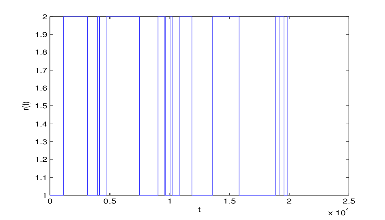
Figure 1: Computer simulation of the paths $\Lambda_{t}.$

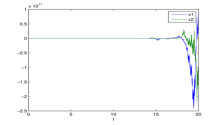
Figure 2: Computer simulation of unstability of $X_{t}$ in (6.8).

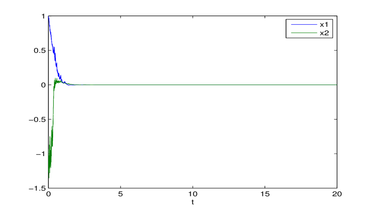
Figure 3: Computer simulation of almost sure stabilization of $X_{t}$ in (6.9).

Appendix A Appendix

Although the latter argument for Theorem 1 is similar to that of [25, Theorem 2.1], we outline the proofs of (3.5) and (3.6) to make the content self-contained.

Claim (3.5). Recall that

$$\sup_{0\leq t<\infty}|X_{t}|<\infty~{}~{}~{}\mbox{a.s.}$$ (A.1)

and that

$$\liminf_{t\rightarrow\infty}V(X_{t})=0~{}~{}~{}~{}~{}\mbox{a.s.}$$ (A.2)

If (3.5) is false, then

$$\mathbb{P}\left\{\limsup_{t\rightarrow\infty}V(X_{t})>0\right\}>0.$$

Therefore, there is a number $\varepsilon>0$ such that

$$\mathbb{P}(\Omega_{1})\geq 3\varepsilon,$$ (A.3)

where $\Omega_{1}=\left\{\limsup_{t\rightarrow\infty}V(X_{t})>2\varepsilon\right\}$.

By (A.1), we find a positive number $M$, which depends on $\varepsilon$, such that

$$\mathbb{P}(\Omega_{2})\geq 1-\varepsilon,$$ (A.4)

where $\Omega_{2}=\left\{\limsup_{t\rightarrow\infty}|X_{t}|<M\right\}$.

From (A.3) and (A.4), we have

$$\mathbb{P}(\Omega_{1}\cap\Omega_{2})\geq 2\varepsilon,$$ (A.5)

We now define a sequence of stopping times,

$$\tau_{M}:=\inf\{t\geq 0:|X_{t}|\geq M\},$$

$$\epsilon_{1}:=\inf\{t\geq 0:V(X_{t})\geq 2\varepsilon\},$$

$$\epsilon_{2k}:=\inf\{t\geq\epsilon_{2k-1}:V(X_{t})\leq\varepsilon\},~{}~{}k=1,2,\cdots$$

$$\epsilon_{2k+1}:=\inf\{t\geq\epsilon_{2k}:V(X_{t})\geq 2\varepsilon\},~{}~{}k=1,2,\cdots$$

where throughout this paper we set $\inf\emptyset=\infty$. From (A.2), we see that if $\omega\in\Omega_{1}\cup\Omega_{2}$, then $\tau_{M}=\infty$ and $\epsilon_{k}<\infty,~{}~{}k=1,2,\cdots.$

By (3.4), we get

$$\infty >\mathbb{E}\int^{\infty}_{0}V(X_{t})\text{\rm{d}}t$$

$$\geq\sum^{\infty}_{0}\mathbb{E}\left[{\bf 1}_{\{\epsilon_{2k-1}<\infty,\epsilon_{2k}<\infty,\tau_{M}=\infty\}}\int^{\epsilon_{2k}}_{\epsilon_{2k-1}}V(X_{t})\text{\rm{d}}t\right]$$

$$\geq\varepsilon\sum^{\infty}_{0}\mathbb{E}\left[{\bf 1}_{\{\epsilon_{2k-1}<\infty,\tau_{M}=\infty\}}(\epsilon_{2k}-\epsilon_{2k-1})\right]$$ (A.6)

where we use the fact $\epsilon_{2k}<\infty$ whenever $\epsilon_{2k-1}<\infty$.

By (H1), we have that there exists a positive constant $L_{M}$ such that

$$\begin{split}&\mathbb{E}\left[{\bf 1}_{\{\epsilon_{2k-1}\wedge\tau_{M}<\infty\}}\sup_{0\leq t\leq T}|X_{\tau_{M}\wedge(\epsilon_{2k-1}+t)}-X_{\tau_{M}\wedge\epsilon_{2k-1}}|^{2}\right]\\ &\leq 2L^{2}_{M}(T+4)T.\end{split}$$ (A.7)

From the uniformly continuous of the function $V$ on the bounded closed ball $\overline{B}_{M}$, we also choose $\delta=\delta(\varepsilon)>0$ such that

$$|V(x)-V(y)|<\varepsilon/2,~{}~{}~{}x,y\in\overline{B}_{M},~{}~{}|x-y|<\delta.$$ (A.8)

Furthermore, we choose $T=T(\varepsilon,\delta,M)$ sufficiently small such that

$$\frac{2L^{2}_{M}(T+4)T}{\delta^{2}}<\varepsilon.$$

From (A.7) and (A.5), we have

$$\begin{split}&\mathbb{P}\bigg{(}\{\epsilon_{2k-1}<\infty,\tau_{M}=\infty\}\\ &\,\,\,\left.\bigcap\{\sup_{0\leq t\leq T}|X_{\epsilon_{2k-1}+t}-X_{\epsilon_{2k-1}}|<\delta\}\right)\geq\varepsilon.\end{split}$$

Using (A.8), we obtain

$$\begin{split}&\mathbb{P}\bigg{(}\{\epsilon_{2k-1}<\infty,\tau_{M}=\infty\}\\ &\,\,\,\left.\bigcap\{\sup_{0\leq t\leq T}|V(X_{\epsilon_{2k-1}+t})-V(X_{\epsilon_{2k-1}})|<\varepsilon\}\right)\geq\varepsilon.\end{split}$$ (A.9)

Set

$$\overline{\Omega}_{k}=\left\{\sup_{0\leq t\leq T}|V(X_{\epsilon_{2k-1}+t})-V(X_{\epsilon_{2k-1}})|<\varepsilon\right\}.$$

We see

$$\epsilon_{2k}(\omega)-\epsilon_{2k-1}(\omega)\geq T$$

when $\omega\in\{\epsilon_{2k-1}<\infty,\tau_{M}=\infty\}\cap\overline{\Omega}_{k}$.

From (A) and (A.9), we derive

$$\begin{split}\infty&>\varepsilon\sum^{\infty}_{0}\mathbb{E}\left[{\bf 1}_{\{\epsilon_{2k-1}<\infty,\tau_{M}=\infty\}}(\epsilon_{2k}-\epsilon_{2k-1})\right]\\ &\geq\varepsilon T\sum^{\infty}_{0}\mathbb{P}(\{\epsilon_{2k-1}<\infty,\tau_{M}=\infty\}\cap\overline{\Omega}_{k})\\ &\geq\epsilon T\sum^{\infty}_{0}\varepsilon=\infty.\end{split}$$ (A.10)

which is a contradiction. Therefore, (3.5) must hold.

Claim (3.6). If (3.6) is false, there exists some $\overline{\omega}\in\Omega_{0}$ such that

$$\limsup_{t\rightarrow\infty}|X_{t}(\overline{\omega})|>0.$$

Then, for some $\varsigma>0,$ there is a subsequence $X_{t_{k}}(\overline{\omega})$ of $X_{t}(\overline{\omega})$ such that $|X_{t_{k}}(\overline{\omega})|\geq\varsigma,~{}~{}k\geq 1.$

By (A.1), there is an increasing subsequence $X_{\overline{t}_{k}}(\overline{\omega})$ of $X_{t_{k}}(\overline{\omega})$ such that $\lim_{k\rightarrow\infty}X_{\overline{t}_{k}}(\overline{\omega})=z\in\mathbb{R}^{n}$ with $|z|\geq\varsigma$. Therefore $\lim_{k\rightarrow\infty}V(X_{\overline{t}_{k}}(\overline{\omega}))=V(z)>0.$

But, from (3.5), we see that this is a contradiction. Therefore, (3.6)holds.

References

- [1]
- [2] Bardet, J. B., Guérin, H., Malrieu, F., Long time behavior of diffusion with Markov switching, ALEA Lat. Am. J. Probab. Math. Stat., 7 (2010), 151–170.
- [3] Berman, A., Plemmons, R.J., Nonnegative matrices in the mathematical sciences, SIAM, Philadelphia, 1994.
- [4] Boyd, S., El Ghaoui, L., Feron, R., Balakrishnan, V., Linear Matrix Inequalities in System and Control Theory, SIAM, Philadelphia, 1994.
- [5] Chen, M.-F., Eigenvalues, inequalities, and Ergodicity Theory, Springer, London, 2005.
- [6] Chen, M., Mao, Y., An Introduction of Stochastic Processes, Higher Education Press, Beijing, 2007.(in Chinese)
- [7] Khasminskii, R., Stochastic Stability of Differential Equations,Second Ed., Springer-Verlag, Berlin, Heideberg, 2012.
- [8] Khasminskii, R., Zhu C., Yin, G., Stability of regime-switching diffusions, Stoch. Proc. Appl., 117 (2007), 1037–1051.
- [9] Lipster, R. S., Shiryayev, A. N., Theory of martingales, Kluwer Academic, 1989.
- [10] Mao, X., Exponential Stability of Stochastic Differential Equations, Marcel Dekker, 1994.
- [11] Mao, X., Stability of stochastic differential equations with Markovian switching, Stoch. Proc. Appl., 79 (1999), 45–67.
- [12] Mao, X., Matasov, A., Piunovskiy, A. B., Stochastic differential delay equations with Markovian switching, Bernoulli, 6 (2000), 73–90.
- [13] Mao, X., Yuan, C., Stochastic Differential Equations with Markovian Switching, Imperial College Press, 2006.
- [14] Mao, X., Stochastic Differential Equations and Applications, Horwood, 2007.
- [15] Mao, X., Shen, Y, Yuan, C., Almost surely asymptotic stability of neutral stochastic differential delay equations with Markovian switching, Stochastic Process. Appl., 118 (2008), 1385–1406.
- [16] Shao, J., Xi, F., Strong ergodicity of the regime-switching diffusion processes, Stoch. Proc. Appl., 123 (2013), 3903–3918.
- [17] Shao, J., Criteria for transience and recurrence of regime-switching diffusions processes, arXiv:1403.3135.
- [18] Shao, J., Ergodicity of regime-switching diffusions in Wasserstein distances, arXiv:1403.0291v1.
- [19] Shao, J., Xi, F., Stability and recurrence of regime-switching diffusion processes, Preprint.
- [20] Shen, Y., Wang, J., Almost sure exponential stability of recurrent neural networks with Markovian switching, IEEE Trans. Neural Netw., 20 (2009), 840–855.
- [21] Xi, F., Feller property and exponential ergodicity of diffusion processes with state-dependent switching, Sci. China Ser. A-Math., 51 (2008), 329–342.
- [22] Xi, F., Yin, G., Stability of regime-switching jump diffusions, SIAM J. Control Optim., 48 (2010), 525–4549.
- [23] Yuan, C., Mao, X., Asymptotic stability in distribution of stochastic differential equations with Markovian switching, Stoch. Proc. Appl., 103 (2003), 277–291.
- [24] Yuan, C., Zou, J., Mao, X., Stability in distribution of stochastic differential delay equations with Markovian switching, Systems Control Lett., 50 (2003), 195–207.
- [25] Yuan, C., Mao, X., Robust stability and controllability of stochastic differential delay equations with Markovian switching, Automatica, 40 (2004), 343–354.
- [26] Yin, G., Zhu, C., Hybrid Switching Diffusions: Properties and Applications, Springer, 2010.
- [27] Zhou, F., Han, Z., Zhang J., Stability analysis of stochastic differential equations with Markovian switching, Syst. Contol Lett. , 61 (2012), 1209–1214.
- [28]