Finding the positive feedback loops underlying multi-stationarity
Abstract
Bistability is ubiquitous in biological systems. For example, bistability is found in many reaction networks that involve the control and execution of important biological functions, such as signalling processes. Positive feedback loops, composed of species and reactions, are necessary for bistability, and generally for multi-stationarity, to occur. These loops are therefore often used to illustrate and pinpoint the parts of a multi-stationary network that are relevant (‘responsible’) for the observed multi-stationarity. However positive feedback loops are generally abundant in reaction networks but not all of them are important for subsequent interpretation of the network’s dynamics.
We present an automated procedure to determine the relevant positive feedback loops of a multi-stationary reaction network. The procedure only reports the loops that are relevant for multi-stationarity (that is, when broken multi-stationarity disappears) and not all positive feedback loops of the network. We show that the relevant positive feedback loops must be understood in the context of the network (one loop might be relevant for one network, but cannot create multi-stationarity in another). Finally, we demonstrate the procedure by applying it to several examples of signalling processes, including a ubiquitination and an apoptosis network, and to models extracted from the Biomodels database.
We have developed and implemented an automated procedure to find relevant positive feedback loops in reaction networks. The results of the procedure are useful for interpretation and summary of the network’s dynamics.
Background
Bistability, and multi-stationarity in general, is ubiquitous in biological systems ranging from biochemical networks to epidemiological and eco-systems [28, 22, 23, 33]. It is considered an important biological mechanism for controlling cellular and bacterial behaviour and developmental processes in organisms, and it is closely linked to the idea of the cell as a decision making unit, where a continuous input is converted to an on/off response corresponding to two distinct states of the cell [19, 24].
The question of bistability therefore arises naturally in many contexts. Many studies aim to demonstrate that in a given biochemical system, bistability can or cannot occur [21, 22, 15, 23, 7]. This has created some interest in formal methods that connect the network structure to the dynamic behaviour of the system, see e.g. [32, 4, 5, 31, 26, 25, 17, 9, 1].
One qualitative network feature has in particular been linked to multi-stationarity, namely the existence of a positive feedback loop. A positive feedback loop consists of a sequence of species such that each species affects the production of another species, either positively or negatively, and such that the number of negative influences is even. The idea of associating positive feedback loops with bistability goes back to Jacob and Monod who introduced it in the context of gene regulatory networks [16]. It was later formalised by Thomas in the form of a conjecture [30], which was finally proved by Soulé [29], see also [13, 18].
Soulé considers dynamical systems of the form
| (1) |
where , is the vector of species concentrations, is the derivative of with respect to time , and is the so-called species-formation rate function, which specifies the instantaneous change in the concentrations.
The work of Soulé is based on the so-called interaction graph [29]. This graph encodes how the variation of one species concentration depends on the concentration of the other species. It is built from the Jacobian matrix of evaluated at a point , such that the non-zero entries of corresponds to directed edges of the graph and the signs of the entries are edge labels. Soulé’s analysis is mainly informative when the signs of the entries are independent of . He proved that the existence of a positive feedback loop in the interaction graph is a necessary condition for to have multiple zeros. In other words, it is a necessary condition for multi-stationarity to exist in the ODE system (1).
Soulé’s approach usually works well when modelling gene networks, but it is often useless when modelling enzymatic signalling networks. In this case, the interaction graph rarely has constant labels. A related line of work, that remedies this short-coming and might be seen as a refinement of Soulé’s work, is based on the so-called directed species-reaction graph (DSR-graph) [6, 3, 2, 32]. If in (1) is obtained from a reaction network, then it decomposes in the form
| (2) |
where is the stoichiometric matrix of the network and the vector of reaction rates. The DSR-graph uses this particular structure.
The DSR-graph is a bipartite graph with nodes labeled by the species and the reactions of the reaction network. There is a signed directed edge from a species to a reaction if the species concentration contributes either positively (positive edge label) or negatively (negative edge label) to the rate of the reaction. There is an edge from a reaction to a species if the stoichiometric coefficient of the species in the reaction is non-zero. In this case the edge is labelled with the sign of the stoichiometric coefficient. Compared to the interaction graph, the DSR-graph makes use of the explicit form of .
The DSR-graph exists in different versions depending on the labelling of the edges (signs versus stoichiometric coefficients) and whether two opposite directed edges between the same node pair are combined into one undirected edge or not [2, 3, 32]. It has been shown that the existence of positive feedback loops in the DSR-graph is a necessary condition for the system (2) to admit multi-stationarity [3].
Based on these results it has become standard to highlight positive feedback loops in multi-stationary reaction networks, eg. [28, 22]. The loops are typically found using intuitive reasoning that might overlook the existence of other relevant positive feedback loops or might select positive feedback loops that are not related to the existence of multi-stationarity. Here we provide a method, based on theoretical considerations, to classify all positive feedback loops of a multi-stationary network into those that are related to the observed multi-stationarity and those that are not. In other words, we determine the positive feedback loops that when broken, multi-stationarity disappears.
The question needs to be understood in the context of the whole network and not in isolation: a particular positive feedback loop that is responsible for multi-stationarity in one network might appear in another network that cannot have multiple steady states.
We present an automated procedure to determine the positive feedback loops that contribute to multi-stationarity. The procedure is based on the injectivity property applied to an ODE system of the form (2), as described in [32]. In this context, we review the proof of the fact that positive feedback loops are necessary for multi-stationarity and how this relates to the DSR-graph. We illustrate the procedure with examples of multi-stationary reaction networks involved in cell signaling. We further consider the networks in the Biomodels database [20] and apply the procedure to all non-injective networks (injective networks cannot be multi-stationary, see below). This provides an overview of the landscape of relevant positive feedback loops occurring in documented reaction networks.
Methods
We use the formalism of Chemical Reaction Network Theory (CRNT) [8]. An ODE system is built from a set of reactions and reaction rates.
Reaction networks
A reaction network, or simply a network, consists of a set of species and a set of reactions of the form:
| (3) |
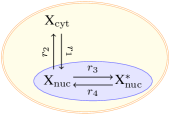
where are nonnegative integers, called the stoichiometric coefficients. As a running example we use the network in Figure 1. It has three species, X, X, X, which are different forms of the Cdk1-cyclin B1 complex, and four reactions [28].
We denote the concentration of the species by lower-case letters . The evolution of the species concentrations with respect to time is modelled as an ODE system in the following way. We let be the stoichiometric matrix of the network:
that is, the -th entry encodes the net production of species in reaction . The vector is called the reaction vector of reaction .
The rate of reaction is a function , where and is the set of possible species concentrations. A typical choice of is mass-action kinetics. In this case
with the convention that . Putting the pieces together provides a model for the evolution of the species concentrations over time:
| (4) |
Returning to Figure 1, we let be the concentrations of X, X, X, respectively. Following [28], one model of the network is:
| (5) | ||||
where are parameters. It takes the form (4) with
| (6) |
| (7) |
and . Observe that the phosphorylation reaction has a reaction rate that depends on both the concentration of the reactant X and the concentration of the product X. We also consider an alternative model in which the rate of X phosphorylation depends on only:
| (8) |
This alternative model is also consistent with the set of reactions in Figure 1, but the third reaction is now independent of the amount of X.
Multi-stationarity
The specific form of (4) implies that the trajectories of the ODE system are confined to the so-called stoichiometric compatibility classes:
where in is the initial condition. That is, the trajectories are restricted to the space spanned by the reaction vectors. Of particular interest is the (relative) interior of , also called the positive stoichiometric compatibility class, given by . Any trajectory that starts in , stays there, but might be attracted towards the boundary.
A reaction network is said to be multi-stationary if there exist two distinct steady states in a positive stoichiometric compatibility class (but not necessarily in all classes). Equivalently, if there exist distinct positive such that and . A network with one positive steady state and one steady state at the boundary is therefore not multi-stationary in this terminology.
Influence matrix
The concept of a positive feedback loop is associated with structural network properties and qualitative features of the reaction rates. Therefore, we assume some regularity on the reaction rates that we encode into an abstract symbolic matrix, called the influence matrix. A feedback loop does not depend on specific parameters or the specific functional form of the reaction rates.
To proceed, we assume that the function is strictly monotone in each variable and define the influence matrix as
where are symbolic variables.
DSR-graph
We define the DSR-graph as a labelled bipartite directed graph with node set and such that:
-
(a)
There is an edge from to with label if .
-
(b)
There is an edge from to with label if .
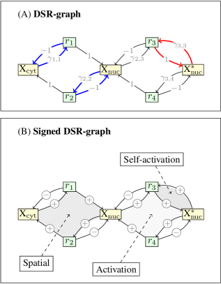
We refer to the signed DSR-graph as the graph identical to the DSR-graph given by (a)-(b), but with the labels replaced by their signs. The (signed) DSR-graph of the running example with as in (6) and as in (9) is shown in Figure 2. The (signed) DSR-graph with as in (10) is identical to that in Figure 2, with the edge from X to removed.
Circuits and nuclei
A circuit in a graph is a sequence of distinct nodes such that there is a directed edge from to for all and one from to . A circuit must involve at least one edge. The label of a circuit , denoted , is the product of the labels of the edges in the circuit. Two circuits are disjoint if they do not have any common nodes.
A circuit with positive label is a positive feedback loop, and similarly, a circuit with negative label is a negative feedback loop. The three positive feedback loops of the running example are shaded in Figure 2B. They correspond to shuttling of the complex between the nucleus and the cytoplasm, activation and deactivation of X, and self-activation of X (the rate of reaction increases with , that is, the production of X increases with the amount of X).
A -nucleus is a collection of disjoint circuits which involves nodes [29]. The label of a -nucleus is the product of the labels of the edges in the nucleus. Let be the number of circuits in the nucleus that have odd (resp. even) number of species nodes and let . The sign of a -nucleus is defined as . That is, if is a disjoint union of circuits, then
| (11) |
In the DSR-graph, any circuit involves an equal number of species and reaction nodes and, hence, an even number of edges. Consider a -nucleus of the DSR-graph. We show that if none of the circuits are positive feedback loops, then the sign of is . Indeed, if all circuits have negative labels, that is, for all , then
Because is a -nucleus, it contains species nodes. Let be the number of species nodes in circuit , such that . We have that is odd for of the circuits and even for of the circuits. Therefore, and
| (12) |
if there are no positive feedback loops in . This result is also in [2], where it is stated using a different terminology.
Injectivity
In this section we study injectivity of the function , (4). In the next section we link this injectivity property for all positive stoichiometric compatibility classes to the non-existence of positive feedback loops in the DSR-graph. With other words, if all feedback loops are negative then the function is injective on all positive stoichiometric compatibility classes. In particular, there cannot exist two distinct points in the same stoichiometric compatibility class such that , that is, the network cannot be multi-stationary.
To decide whether the function is injective on all positive stoichiometric compatibility classes for any with given influence matrix , we rely on a method previously developed by us [11, 32, 12]. We will now explain this method.
Given a pair of matrices , we define a polynomial of degree , in as many variables as there are non-zero entries of . For this, let and let be a basis of , which we assume to be Gauss-reduced. Further, let be the indices of the first non-zero entries of , respectively. We define a symbolic matrix, , by replacing the -th row of with (cf. [32, Section 5]). The polynomial is defined as
which can be written as a sum of terms depending on the variables , by expanding the determinant. Each non-zero term is of the form where is a coefficient and all , respectively , are distinct.
It is a result of [32, 12] that if is not identically zero and all non-zero coefficients of have the same sign, then the function is injective on each positive stoichiometric compatibility class and, hence, the network cannot be multi-stationary. As a consequence, has coefficients of opposite sign whenever the network is multi-stationary. If the coefficients do not have the same sign, then the network might be multi-stationary, but it cannot be concluded from the test.
Consider the matrix given in (6) and in (9). We choose as a basis of and obtain
| (13) | ||||
There are both positive and negative terms, hence multi-stationarity cannot be excluded. For in (10), the polynomial is obtained from (13) by setting ,
| (14) |
In this case all terms have the same sign and thus, the network cannot be multi-stationary. This holds for any choice of rate functions with influence matrix .
The polynomial and circuits
In this section we link injectivity and the polynomial to positive feedback loops. It is shown in [32] that each term of the polynomial can be identified with a collection of disjoint unions of circuits in the DSR-graph . Specifically, given subsets of cardinality , let be the set of -nuclei of with node set . Then
| (15) |
where the sets in the sum have cardinality (cf. [32, Section 11]).
When is derived from a “reasonable” reaction network, the predominant sign of the coefficients is . This is because, for most reactions, the species in the reactant complex will have positive influence on the reaction rate, and the species in the product complex will have negative influence; if they influence the reaction at all. Consequently, if the network is multi-stationary, then has some terms with the wrong sign, that is, with sign . Since whenever does not contain positive feedback loops (12), we conclude that the network must contain positive feedback loops in order to be multi-stationary.
Based on the above considerations, we develop a procedure to extract the positive feedback loops that correspond to terms with the wrong sign in . Fix a non-zero term of the polynomial , say
| (16) |
( is positive) and consider the following edges from species to reactions
The -nuclei corresponding to the term (16) must contain these edges. Therefore, we add to these edges all possible choices of edges from reactions to species such that the resulting graph is a -nucleus. We keep only the nuclei for which the sign of is . The positive feedback loops in these nuclei are those that do contribute to the existence of multiple steady states. Indeed, if all these loops are broken, then the network cannot be multi-stationarity. We find these loops in the signed DSR-graph.
For example, consider the polynomial in (13) and the DSR-graph shown in Figure 2. In this case, the rank of is , and hence we focus on the negative terms since . These are and . The corresponding -nuclei are depicted in Figure 2(A): there are two 4-nuclei obtained as the union of the red circuit and one of the two blue circuits. The only positive feedback loop that appears is therefore the self-activation positive feedback loop, and this is the only loop that is related to the observed multi-stationarity. The other two positive feedback loops (termed the spatial and the activation loop, respectively in Figure 2(B)) are therefore not relevant for the observed multi-stationarity.
Automated procedure
The procedure to select positive feedback loops that contribute to multi-stationarity consists of the following steps.
-
1.
For a network with stoichiometric matrix of rank and influence matrix , compute and select the terms with sign .
-
2.
Construct the DSR-graph. For each selected term of with the wrong sign, determine the corresponding -nuclei of the DSR-graph that have the wrong sign.
-
3.
For each of the nuclei, select the connected components that form positive feedback loops.
These steps have been implemented in Maple and the script is available upon request. The procedure might fail for practical reasons (such as lack of computational memory) if the number of species and reactions is too big. In our experience, this number depends heavily on the sparsity of the influence matrix [12].
Examples
We have applied the procedure to several multi-stationary networks. These examples are also in the Maple script, together with some other systems such as the three-site phosphorylation system.
Ring1B/Bmi1 ubiquitination system
We consider an ODE model of histone H2A ubiquitination that involves the E3 ligases Ring1B and Bmi1 [23]. When degradation of species is not taken into account, the model has species and reactions. We let B and B denote the protein Bmi1 in isolation and targeted for degradation by ubiquitination, respectively. The protein Ring1B is denoted by R, and Rub, R, R denote three different forms of self-ubiquitinated R, with R being the form targeted for degradation. Bmi1 and Ring1B form a complex Z, that also might be ubiquitinated, Zub. Finally, Ring1B (either alone or in the complex Z) is responsible for the ubiquitination of the histone H2A, with states H, Hub.
The reactions describing the mechanism are [23]:
| B | R | ||||||
| Z | R | ||||||
| H | |||||||
We let denote the concentrations of B, B, R, R, Rub, R, Z, Zub, H, Hub, respectively. The associated reaction rates are [23]:
where are constants.
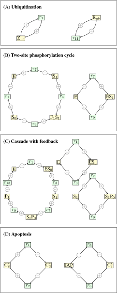
Self-ubiquitination of B is taken into account in the rate functions and for reactions and , respectively. These incorporate a positive influence from the reaction products. With these specific rate functions, the system is multi-stationary [23]. We apply the automated procedure to find positive feedback loops and obtain the circuits depicted in Figure 3(A). In [23], it is postulated that self-ubiquitination of Z and R are crucial steps for the emergence of multiple steady states, and we confirm the statement here.
Phosphorylation systems
We have analysed different networks of signal transmission based on phosphorylation. We consider models for sequentially distributed phosphorylation and dephosphorylation cycles and some modifications of these, see e.g. [10, 14].
We consider first a two-site sequential phosphorylation cycle for a substrate S, where phosphorylation of the two sites is catalysed distributively by a kinase E, and dephosphorylation of the two sites uses different phosphatases F1, F2. Assuming a Michaelis-Menten mechanism, the reaction network consists of the following reactions:
In S0, S1, S2 the subindex denotes the number of phosphorylated sites. With mass-action kinetics, this system is multi-stationary [22, 10]. However, the positive feedback loops that can account for the observed multi-stationarity are not trivial.
We apply the automated procedure and obtain the positive feedback loops given in Figure 3(B). The first of the two loops has two edges with negative labels. It implies that S0 and S1 enhance their own production. Indeed, because S0 and S1 both compete for the same kinase, an increase in S0 increases the rate of reaction , which in turn lowers the amount of available enzyme E. This implies that reaction slows down and hence S1 is consumed at a slower rate. The circuit closes through the reactions and , which shows that an increase in S1 implies an increase in S0.
These type of loops are recurrent in phosphorylation motifs. It is worth emphasising that the loops do not have independent meaning outside to network. Another network with the same positive feedback loop might not be multi-stationarity. This is apparent from the second positive feedback loop in Figure 3(B), which is present whenever a Michaelis-Menten enzymatic mechanism is considered.
Signalling cascades
We consider a 2-layer cascade with an explicit positive feedback. The first layer is a phosphorylation cycle with kinase E, phosphatase F1, and phosphorylated and unphosphorylated substrate S0, S1. The second layer has kinase S1, phosphatase F2, and phosphorylated and unphosphorylated substrate P0, P1. Assuming a Michaelis-Menten mechanism, the reaction network consists of the following reactions:
The automated procedure finds three positive feedback loops, as shown in Figure 3(C). The first loop is expected and appears because the product of the second layer, P1, activates the kinase of the first layer, E. The other two loops are similar to those in Figure 3(C).
Apoptosis
We finally consider a basic model of caspase activation for apoptosis [7]:
| IAP | |||||
With mass-action kinetics, this network is multi-stationary [7] and has two relevant positive feedback loops, Figure 3(D). The second loop consists of two species, each with positive influence on a reaction rate, while at the same time, decreasing the amount of the other.
Analysis of the Biomodels database
We investigated the models in the database PoCaB [27], which consists of 365 models from the publicly available database Biomodels [20] (see also the page http://www.ebi.ac.uk/biomodels-main/). The database PoCaB contains pre-computed stoichiometric matrices, mass-action exponent matrices, and kinetic data from the selected models.
In a previous paper [12] we extracted influence matrices of the reported kinetics. Of the 365 networks, 323 have strictly monotone kinetics such that the influence matrix is well defined. On these 323 networks we ran the injectivity method and ended up with a total of 64 non-injective networks, excluding 27 very large networks where the injectivity method failed (as described in [12]). Non-injectivity is a prerequisite for being multi-stationary.
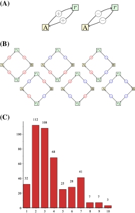
We applied the automated procedure on the 64 networks to determine the positive feedback loops. We obtained a total of 341 different positive feedback loops with size distribution shown in Figure 4(C). Most loops involve only 2 or 3 species (112 and 108 loops out of 341, respectively). In Figure 4(A-B), we show the positive feedback loops involving one or two species and conclude that all possible types occur in the database. However, for two species, their frequencies vary from 9 to 35 (out of 108), indicating that the motifs are not equally represented in the database (Pearson’s chi-square test, ). For one species, there appears to be no difference (). We show in Table 1 the most frequent positive feedback loops for different number of species nodes.
| Motif | Frequency | |
|---|---|---|
| 2 | 23/112 = 0.21 | |
| 35/112 = 0.31 | ||
| 3 | 19/108 = 0.18 | |
| 18/108 = 0.17 | ||
| 4 | 15/68 = 0.22 | |
| 15/68 = 0.22 | ||
| 14/68 = 0.21 | ||
| 5 | 9/25 = 0.36 | |
| 7/25 = 0.28 | ||
| 6 | 6/28 = 0.21 | |
| 7/28 = 0.25 | ||
| 7 | 14/41 = 0.34 |
Discussion
We have presented an automated procedure to find the positive feedback loops in a multi-stationary network. The procedure relies on structural and qualitative features of the network together with a kinetics, and it is insensitive to the specific form of the rate functions. Only positive feedback loops that are contributing to the multi-stationarity of the network are reported, excluding those positive feedback loops that are not relevant.
Whether a loop is relevant or not, depends on the entire DSR-graph of the network (that is, the reactions and the influence matrix) and not just on the loop itself. In this sense, being a positive feedback loop related to an observed multi-stationarity, is a context or network dependent property. This fact has also been observed in [6, 3, 2]. In these papers, it is shown that the existence of a positive feedback loop fulfilling a certain extra condition is a requirement for multi-stationarity to occur. Specifically, the loop must either intersect another positive feedback loop in a specific way (called an S-to-R intersection) or fulfil a certain condition on the labels (called an s-cycle). The first possibility is network dependent. It is worth mentioning that there can be positive feedback loops that are s-cycles or that intersect another positive feedback loop in an S-to-R intersection without being relevant for the observed multi-stationarity. This is the case for most of the examples presented here. For example, the apoptosis network has another positive feedback loop, YY (all edges are positive), which intersects the loop on the right side in Figure 3(D) in an S-to-R intersection.
The property of network dependence is further illustrated in Figure 2(A)-(B), where the procedure is applied to the reaction network in Figure 1 with influence matrix given by (9). The network models translocation and phosphorylation of a cyclin dependent kinase X in the onset of mitosis. Only one of the three positive feedback loops shown in Figure 2(B) can be associated with multi-stationarity in the model, namely the self-activating loop that stimulates the creation of phosphorylated X in the nucleus. In [28], it is argued by different means than in this paper, that the spatial redistribution of the cyclin dependent kinase is important for creating the observed bistability. In contrast, our results suggest that the observed bistability is due to the self-activation loop of the phosphorylated complex in the nucleus.
The presented procedure cannot establish whether a reaction network is multi-stationary or not. Other means will here be required. If the procedure is applied to a reaction network that might or might not be multi-stationary, then the absence of positive feedback loops implies that the network cannot be multi-stationary, whereas the presence of positive feedback loops leaves the question open.
Whether a positive feedback loop found by the procedure is important in a biological or experimental context, is not addressed in this paper, but must be established in other ways, for example by experimental verification. A reaction network might only be multi-stationary for very specific choices of reaction rates, which might not be relevant in a particular experimental setting. As the procedure is parameter independent, any such verification and subsequent interpretation is beyond the scope of the procedure.
Acknowledgements
CW was supported by the Danish Research Council, the Lundbeck Foundation (Denmark) and the Carlsberg Foundation (Denmark). EF was supported by project MTM2012-38122-C03-01/FEDER from the Ministerio de Economía y Competitividad (Spain), and the Lundbeck Foundation (Denmark). This paper was completed while the authors were visiting the Isaac Newton Institute in Cambridge, UK.
References
- [1] D. Angeli, P. De Leenheer, and E. Sontag. Graph-theoretic characterizations of monotonicity of chemical networks in reaction coordinates. J. Math. Biol., 61:581–616, 2010.
- [2] M. Banaji and G. Craciun. Graph-theoretic approaches to injectivity and multiple equilibria in systems of interacting elements. Commun. Math. Sci., 7(4):867–900, 2009.
- [3] M. Banaji and G. Craciun. Graph-theoretic criteria for injectivity and unique equilibria in general chemical reaction systems. Adv. Appl. Math., 44:168–184, 2010.
- [4] C. Conradi and D. Flockerzi. Switching in mass action networks based on linear inequalities. SIAM J. Appl. Dyn. Syst., 11(1):110–134, 2012.
- [5] G. Craciun and M. Feinberg. Multiple equilibria in complex chemical reaction networks. I. The injectivity property. SIAM J. Appl. Math., 65(5):1526–1546, 2005.
- [6] G. Craciun and M. Feinberg. Multiple equilibria in complex chemical reaction networks. II. The species-reaction graph. SIAM J. Appl. Math., 66(4):1321–1338, 2006.
- [7] T. Eissing, H. Conzelmann, E. D. Gilles, F. Allgower, E. Bullinger, and P. Scheurich. Bistability analyses of a caspase activation model for receptor-induced apoptosis. J. Biol. Chem., 279(35):36892–36897, 2004.
- [8] M. Feinberg. Lectures on chemical reaction networks. Available online at http://www.crnt.osu.edu/LecturesOnReactionNetworks, 1980.
- [9] M. Feinberg. Chemical reaction network structure and the stability of complex isothermal reactors I. The deficiency zero and deficiency one theorems. Chem. Eng. Sci., 42(10):2229–68, 1987.
- [10] E. Feliu and C. Wiuf. Enzyme-sharing as a cause of multi-stationarity in signalling systems. J. R. S. Interface, 9(71):1224–32, 2012.
- [11] E. Feliu and C. Wiuf. Preclusion of switch behavior in reaction networks with mass-action kinetics. Appl. Math. Comput., 219:1449–1467, 2012.
- [12] E. Feliu and C. Wiuf. A computational method to preclude multistationarity in networks of interacting species. Bioinformatics, 29:2327–2334, 2013.
- [13] J. L. Gouze. Positive and negative circuits in dynamical systems. J. Biol. Syst., 6:11–15, 1998.
- [14] J. Gunawardena. Distributivity and processivity in multisite phosphorylation can be distinguished through steady-state invariants. Biophys. J., 93:3828–3834, 2007.
- [15] H. A. Harrington, E. Feliu, C. Wiuf, and Stumpf M. P. H. Cellular compartments cause multistability in biochemical reaction networks and allow cells to process more information. Biophys. J., 104:1824–1831, 2013.
- [16] F. Jacob and J. Monod. Genetic regulatory mechanisms in the synthesis of proteins. J. Mol. Biol., 3:318–356, 1961.
- [17] B. Joshi and A. Shiu. Atoms of multistationarity in chemical reaction networks. J. Math. Chem., 51(1):153–178, 2013.
- [18] M. Kaufman, C. Soulé, and R. Thomas. A new necessary condition on interaction graphs for multistationarity. J. Theor. Biol., 248:675–685, 2007.
- [19] S. Legewie, N. Bluthgen, R. Schäfer, and H. Herzel. Ultrasensitization: switch-like regulation of cellular signaling by transcriptional induction. PLoS Computational Biology, 1(5):e54, 2005.
- [20] C. Li, M. Donizelli, N. Rodriguez, H. Dharuri, L. Endler, V. Chelliah, L. Li, E. He, A. Henry, M. I. Stefan, J. L. Snoep, M. Hucka, N. Le Novère, and C. Laibe. BioModels Database: An enhanced, curated and annotated resource for published quantitative kinetic models. BMC Systems Biology, 4:92, 2010.
- [21] D. Liu, X. Chang, Z. Liu, L. Chen, and R. Wang. Bistability and oscillations in gene regulation mediated by small noncoding rnas. PLoS ONE, 6(3):e17029, 2011.
- [22] N. I. Markevich, J. B. Hoek, and B. N. Kholodenko. Signaling switches and bistability arising from multisite phosphorylation in protein kinase cascades. J. Cell Biol., 164:353–359, 2004.
- [23] L. K. Nguyen, J. Muñoz-García, H. Maccario, A. Ciechanover, W. Kolch, and B. N. Kholodenko. Switches, excitable responses and oscillations in the ring1b/bmi1 ubiquitination system. PLoS Comput. Biol., 7(12):e1002317, 2011.
- [24] S. Palani and C.A. Sarkar. Synthetic conversion of a graded receptor signal into a tunable, reversible switch. Mol. Sys. Biol., 7:480, 2011.
- [25] M. Pérez Millán, A. Dickenstein, A. Shiu, and C. Conradi. Chemical reaction systems with toric steady states. Bull. Math. Biol., 74:1027–1065, 2012.
- [26] D.A. Rand, B.V. Shulgin, D. Salazar, and A.J. Millar. Design principles underlying circadian clocks. J. R. Soc. Interface, 119–130:2874–2880, 2004.
- [27] S. S. Samal, H. Errami, and A. Weber. Pocab: A software infrastructure to explore algebraic methods for bio-chemical reaction networks. Lecture Notes in Computer Science, 7442:294–307, 2012.
- [28] S. D. Santos, R. Wollman, T. Meyer, and Ferrell J. E. Jr. Spatial positive feedback at the onset of mitosis. Cell, 149(7):1500–1513, 2012.
- [29] C. Soulé. Graphic requirements for multistationarity. ComPlexUs, 1:123–133, 2003.
- [30] R. Thomas. On the relation between the logical structure of systems and their ability to generate multiple steady states or sustained oscillations. Springer series in Synergetics, 9:180–183, 1981.
- [31] J.J. Tyson, K.C. Chen, and B. Novak. Sniffers, buzzers, toggles and blinkers: dynamics of regulatory and signaling pathways in the cell. Curr. Opin. Cell. Biol., 15:221–231, 2003.
- [32] C. Wiuf and E. Feliu. Power-law kinetics and determinant criteria for the preclusion of multistationarity in networks of interacting species. SIAM J. Appl. Dyn. Syst., 12:1685–1721, 2013.
- [33] V. P. Zhdanov. Bistability in gene transcription: interplay of messenger RNA, protein, and nonprotein coding RNA. Biosystems, 95(1):75–81, 2009.