Thermal transport in out-of-equilibrium quantum harmonic chains

Abstract

We address the problem of heat transport in a chain of coupled quantum harmonic oscillators, exposed to the influences of local environments of various nature, stressing the effects that the specific nature of the environment has on the phenomenology of the transport process. We study in detail the behavior of thermodynamically relevant quantities such as heat currents and mean energies of the oscillators, establishing rigorous analytical conditions for the existence of a steady state, whose features we analyze carefully. In particular, we assess the conditions that should be faced to recover trends reminiscent of the classical Fourier law of heat conduction and highlight how such a possibility depends on the environment linked to our system.

Understanding the transport properties in open systems in contact with several energy or particle baths represents a challenge for nonequilibrium physics. Ideally, one would like to characterize and even calculate explicitly the statistics of the energy and particle currents, similarly to what can be done with observables in ensembles at equilibrium. However the properties of the currents in out-of-equilibrium systems depends strongly on the bath properties, and on the characteristics of the system-bath coupling. In this context, chains of oscillators have been extensively used as microscopic models for heat conduction and, in general, for out-of-equilibrium systems dhar ; livi ; hans12 ; hans14 to investigate the behavior of the thermal conductivity for different interaction potentials between the oscillators, different bath properties, or different system-bath couplings livi ; dhar .

The Fourier law of heat conduction implies that the heat current $J$ flowing throughout a system under a temperature gradient scales as the inverse of the system size $L$, i.e., $J\sim 1/L$. In the classical case, it is known that this law is violated in 1D homogeneous harmonic systems rieder ; hans12 where heat is carried by freely propagating elastic waves, while the current scales with the system size in presence of anharmonicity or disorder either in mass or in the coupling constant. Although the transport is anomalous ($J\sim 1/L^{\alpha}$, with $\alpha\neq 1$) in these cases, the Fourier law is finally restored only in presence of a external substrate potential dhar or in the presence of a locally attached energy-conserving reservoirs for each oscillator landi .

Quantum mechanically, a realistic description of a quantum medium for the transport of heat would imply the use of an explicitly open-system formalism and the introduction of system-environment interactions. In this context, it is interesting to identify the conditions, if any, under which heat transport across a given quantum system can be framed into the paradigm of Fourier law. Finding a satisfactory answer to this question is certainly not trivial, in particular in light of the ambiguities that the validity of Fourier law has encountered even in the classical scenario rieder ; hans12 .

In the quantum scenario, significant studies are embodied in the work by Martinez and Paz martinez , who show the emergence of the three laws of thermodynamics in arbitrary networks evolving under a quantum Brownian master equation. This has been applied in Ref. freitas to show that the heat transport in this system is anomalous. Assadian et al. assadian , on the other hand, have addressed a chain of oscillators described by a Lindblad master equation, finding that a Fourier-like dependence on the system size can be observed for very long harmonic chains in the presence of dephasing. Our work is also concerned with heat transfer in harmonic chains but the physical environment surrounding the chain is what differentiates our work from the ones previously cited. Basically, we include the possibility of establishing a temperature gradient using purely diffusive reservoirs, something not yet considered in the literature. Additionally, we further explore the effect of having the chain members locally attached to regular thermal baths at different temperatures.

In this paper, we contribute to such research efforts by studying a general quadratic model for the dynamics of the system that, in turn, are affected by individual thermal reservoirs and exposed to the temperature gradient generated by all-diffusive environments. Our approach is able to pinpoint the origins of the specific energy distributions observed by varying the operating conditions of the system and thus identify the role played, respectively, by the diffusive and thermal reservoirs in the process of heat transport. We find working configurations that deviate substantially from the expectations arising from Fourier law and single out scenarios that are strictly adherent to such a paradigm, thus remarking the critical role played by the nature of the environment affecting the medium in the establishment of the actual mechanism for heat transport.

The remainder of this paper is organized as follows. In Sec. I we introduce the formalism used to address the dynamics of the system. The general scenario addressed in our investigation is described in Sec. II, while the thermodynamic properties and phenomenology of heat currents are analyzed in Sec. III. Section IV is devoted to the analysis of a few significant cases that help us addressing the deviations from (and adherences to) Fourier law. Finally, Sec. V is devoted to the conclusions.

I Tools and notation

In this section we will consider a large class of systems with a generic number of degrees of freedom $n$. Let us define the operator

$$\hat{x}=(\hat{q}_{1},...,\hat{q}_{n},\hat{p}_{1},...\hat{p}_{n})^{\dagger},$$ (1)

which is the column vector composed by $n$ generalized coordinates together with $n$ canonical conjugate momenta. It is possible to express the canonical commutation relations involving coordinates and momenta compactly as $[\hat{x}_{j},\hat{x}_{k}]=i\hbar\,\mathsf{J}_{jk}$ with ${\sf J}_{ij}$ the elements of the symplectic matrix

$$\mathsf{J}=\left(\!\!\begin{array}[]{rc}{\bf 0}_{n}&\mathsf{I}_{n}\\ -\mathsf{I}_{n}&{\bf 0}_{n}\end{array}\!\!\right).$$ (2)

Here $\mathsf{I}_{n}$ and ${\bf 0}_{n}$ are the $n$ dimensional identity and zero matrix, respectively. In the remainder of these notes, we will be dealing with quadratically coupled harmonic oscillators. In this scenario, the use of first and second moments of $\hat{x}$ provides a powerful tool for the description of the physically relevant quantities involved in the evolution of the system. We thus introduce the mean value (MV) vector $\langle\hat{x}\rangle_{t}={\rm Tr}\left[\hat{x}\hat{\rho}(t)\right]$ and the covariance matrix (CM) ${\bf V}$ of elements

$$\mathbf{V}_{\!jk}(t)=\tfrac{1}{2}{\rm Tr}\left[\left\{\hat{x}_{j}-\langle\hat{x}_{j}\rangle_{t},\hat{x}_{k}-\langle\hat{x}_{k}\rangle_{t}\right\}\hat{\rho}(t)\right].$$ (3)

The focus of our work will be the study of a nearest neighbor-coupled harmonic chain whose $n$ elements are in contact with (individual) local reservoirs at finite temperature. The evolution of the chain can thus be described, in general, through the Lindblad master equation

$$\frac{d\hat{\rho}}{dt}=-\frac{i}{\hbar}[\hat{H},\hat{\rho}]-\frac{1}{2\hbar}\!\sum_{m}(\{\hat{L}_{m}^{\dagger}\hat{L}_{m},\hat{\rho}\}-2\hat{L}_{m}\hat{\rho}\hat{L}_{m}^{\dagger})$$ (4)

with the following general form of a quadratic Hamiltonian and linear Lindblad operators

$$\hat{H}=\frac{1}{2}\hat{x}\cdot\mathbf{H}\hat{x}+\xi\cdot\mathsf{J}\hat{x}+H_{0},~{}~{}\hat{L}_{m}=\lambda_{m}\cdot\mathsf{J}\hat{x}+\mu_{m},$$ (5)

where $\mathbf{H}$ is the adjacency matrix of the Hamiltonian, $\xi\in\mathbb{R}^{2n}$ is a column vector encompassing possible position and momentum displacements, $H_{0}\in\mathbb{R}$ represents a possible energy offset, and $\lambda_{m}\in\mathbb{C}^{2n}$ contains the coupling strengths between a given element of the chain and the respective reservoir. Finally, $\mu_{m}\in\mathbb{C}$ are constants endnote2 . Using such a general description of the coherent and incoherent part of the evolution, we can straightforwardly work out the dynamical equations of motion for both $\langle\hat{x}\rangle_{t}$ and the CM by calculating their time derivative and using the state evolution provided by Eq. (4) as nicacio

$$\frac{d\langle\hat{x}\rangle_{t}}{dt}=\xi-\eta+{\bf\Gamma}\langle\hat{x}\rangle_{t},~{}~{}\frac{d\mathbf{V}}{dt}={\bf\Gamma}\mathbf{V}+\mathbf{V}{\bf\Gamma}^{\top}+{\bf D},$$ (6)

where we have introduced $\eta=\sum_{m}{\rm Im}(\mu_{m}^{\ast}\,\lambda_{m})$ and

$${\bf\Gamma}=\mathsf{J}\mathbf{H}-{\rm Im}{\bf\Upsilon}\mathsf{J},~{}~{}~{}~{}{\bf D}=\hbar\,{\rm Re}{\bf\Upsilon},$$ (7)

which are defined in terms of the decoherence matrix ${\bm{\Upsilon}}=\sum_{m}\lambda_{m}\lambda_{m}^{\dagger}$. By definition, we have ${\rm Im}{\bf\Upsilon}^{\top}=-{\rm Im}{\bf\Upsilon}$ and ${\bf D}={\bf D}^{\top}\geq 0$.

For time independent problems, Eqs. (6) can be solved exactly as

$$\langle\hat{x}\rangle_{t} ={\rm e}^{{\bf\Gamma}t}\langle\hat{x}\rangle_{0}+{\bf\Gamma}^{-1}\left({\rm e}^{{\bf\Gamma}t}-\mathsf{I}_{2n}\right)(\xi-\eta),$$ (8)

$${\bf V}(t) ={\rm e}^{{\bf\Gamma}t}\,{\bf V}\!_{0}\,{\rm e}^{{\bf\Gamma}^{\!\top}t}+\int_{0}^{t}\!dt^{\prime}\,{\rm e}^{{\bf\Gamma}t^{\prime}}\,{\bf D}\,{\rm e}^{{\bf\Gamma}^{\!\top}t^{\prime}}$$

with $\langle\hat{x}\rangle_{0}$ and ${\bf V}\!_{0}$ the MV and CM of the initial state, respectively. The steady-state (or fixed-point) solutions of such equations can be found by imposing ${d}\mathbf{V}/{dt}={d}\langle\hat{x}\rangle_{t}/{dt}=0$, which are equivalent to the conditions (in what follows, the subscript $\star$ will be used to indicate steady-state values)

$$\langle\hat{x}\rangle_{\star}=-{\bf\Gamma}^{-1}(\xi-\eta),~{}~{}{\bf\Gamma}\mathbf{V}_{\!\star}+\mathbf{V}_{\!\star}{\bf\Gamma}^{\top}+{\bf D}=0.$$ (9)

The equation satisfied by ${\bf V}_{\!\star}$ is of the stationary Lyapunov form horn that, under the conditions above, admits a unique positive-definite solution iff the eigenvalues of $\bf\Gamma$ have positive real parts. In this case, we find

$${\bf V}_{\!\star}=\lim_{t\to\infty}{\bf V}(t)=\int_{0}^{\infty}\!\!dt\,{\rm e}^{{\bf\Gamma}t}\,{\bf D}\,{\rm e}^{{\bf\Gamma}^{\!\top}\!t}\,.$$ (10)

For-time dependent $\bf H$, $\xi$, $\eta$, and $\lambda_{m}$, the form of $\langle\hat{x}\rangle_{\star}$ in Eq. (9) is no longer valid and the conditions over the Lyapunov equation for ${\bf V}_{\!\star}$ must hold at each instant of time.

Note that, in order to deduce Eqs. (6), (8), and (10), we did not need to make any assumption on the initial state of the system but only use the quadratic and linear structure of Eq. (5) and (4), respectively. The rest of our analysis will focus on the dynamics of thermodynamically relevant quantities such as currents and energy.

II The System and its dynamics

We can now start analyzing explicitly the system that we have in mind. We consider the chain of oscillators depicted in Fig. 1, each interacting with its own thermal reservoir at temperature $T_{k},\,k=1,...,n$. The Hamiltonian of the chain arises from the application of the rotating-wave approximation on a nearest-neighbour Hooke-like coupling model, which gives us

$$\hat{H}=\hbar\omega\sum_{j=1}^{n}\hat{a}_{j}^{\dagger}\hat{a}_{j}+2\hbar\Omega\sum_{j=1}^{n-1}(\hat{a}_{j}^{\dagger}\hat{a}_{j+1}+\hat{a}_{j+1}^{\dagger}\hat{a}_{j}),$$ (11)

where $\omega$ and $\Omega$ are the frequency of the oscillators and their mutual coupling rate respectively, and $\hat{a}_{j}=(\hat{q}_{j}+i\hat{p}_{j})/{\sqrt{2\hbar}}$ is the creation operator of the $j^{\rm th}$ oscillator. Using the notation introduced before, $\hat{H}$ can be written as in Eq. (5) with $\xi=H_{0}=0$ and the adjacency matrix $\mathbf{H}={\boldsymbol{H}}\oplus{\boldsymbol{H}}$, where

$${\boldsymbol{H}}_{\!jk}=\omega\,\delta_{jk}+\Omega\,(\delta_{j\,k+1}+\delta_{j\,k-1})$$ (12)

and $\delta_{jk}$ is the Kronecker symbol.

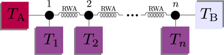
Figure 1: (Color online) Schematic representation of the system. A chain of coupled harmonic oscillators interacting according to an RWA model.

The coupling between a given oscillator and the respective thermal reservoir is described by the Lindblad operators endnote3

$$\hat{L}_{k}=\sqrt{\hbar\zeta_{k}(\bar{N}_{k}+1)}\,\hat{a}_{k},~{}~{}\hat{L}_{k}^{\prime}=\sqrt{\hbar\zeta_{k}\bar{N}_{k}}\,\hat{a}_{k}^{\dagger},$$ (13)

where $\zeta_{k}\geq 0$ is the bath-oscillator coupling and $\bar{N}_{k}$ is the mean occupation number of the reservoirs at temperature $T_{k}$. This choice allows us to make the identifications

$${\lambda}_{k} = \sqrt{\frac{\zeta_{k}}{2}(\bar{N}_{k}+1)}\,(\underbrace{0,...,0}_{k-1},i,\underbrace{0,...,0}_{n-1},-1,\underbrace{0,...,0}_{n-k})^{\top},$$

$$\lambda^{\prime}_{k} = \sqrt{\frac{\zeta_{k}}{2}\bar{N}_{k}}\,(\underbrace{0,...,0}_{k-1},-i,\underbrace{0,...,0}_{n-1},-1,\underbrace{0,...,0}_{n-k})^{\top}.$$ (14)

We now make the explicit assumption that the first and last oscillator in the chain are also affected by two additional reservoirs, which we label ${\rm A}$ and ${\rm B}$, having temperatures $T_{\rm A}\geq T_{\rm B}\gg T_{k}$. This allows us to approximate $\bar{N}_{l}+1\approx\bar{N}_{l}$ for $l={\rm A},{\rm B}$. Therefore, such baths contribute with

$$\lambda^{\prime}_{\rm A} =\lambda^{\ast}_{\rm A}=\sqrt{\frac{\zeta_{\rm A}}{2}\bar{N}_{\rm A}}\,(i,\underbrace{0,...,0}_{n-1},-1,\underbrace{0,...,0}_{n-1})^{\dagger},$$ (15)

$$\lambda^{\prime}_{\rm B} =\lambda^{\ast}_{\rm B}=\sqrt{\frac{\zeta_{\rm B}}{2}\bar{N}_{\rm B}}\,(\underbrace{0,...,0}_{n-1},i,\underbrace{0,...,0}_{n-1},-1)^{\dagger}.$$

We are now in a position to give some motivations for the specific choice of the system to study. In a realistic scenario, the impossibility to achieve full isolation leads one to take into account the external and uncontrollable influences from the environment over the evolution of a system. In our case such disturbances are represented by the $n$ thermal reservoirs attached to each oscillator of the chain. On the other hand, as we aim at studying heat transport across the system, we need to set a temperature gradient, which is imposed, in our setting, by the external end-chain baths. As such gradient is supposed to be the leading mechanism for the transport process, it is reasonable to assume that $T_{A,B}$ are the largest temperatures across the system.

We can now go back to the formal description of the system and write the decoherence matrix as ${\bf\Upsilon}={\bf\Upsilon}^{({\rm A})}+{\bf\Upsilon}^{({\rm B})}+\sum_{k=1}^{n}{\bf\Upsilon}^{(k)}$ with

$${\bf\Upsilon}^{(k)}=\lambda_{k}\lambda_{k}^{\dagger}+\lambda_{k}^{\prime}\lambda_{k}^{\prime\dagger}~{}~{}~{}(k=1,\dots,n),$$ (16)

$${\bf\Upsilon}^{(l)}=2\,{\rm Re}(\lambda_{l}\lambda_{l}^{\dagger})~{}~{}~{}~{}~{}~{}~{}~{}~{}(l={\rm A},{\rm B}).$$

As the contribution given by the reservoirs ${\rm A}$ and ${\rm B}$ to the dynamics is all in the matrix $\mathbf{D}$ of Eq. (7), we refer to them as all-diffusive.

In order to simplify our analysis without affecting its generality, we now take $\zeta_{k}=\zeta$. From Eq. (12) and the expression found for ${\bm{\Upsilon}}$, we rewrite (7) as

$${\bf\Gamma}=-\begin{pmatrix}\frac{\zeta}{2}\,\mathsf{I}_{n}&-{\boldsymbol{H}}\\ {\boldsymbol{H}}&\frac{\zeta}{2}\,\mathsf{I}_{n}\end{pmatrix},\,\,\,{\bf D}=\frac{\hbar\zeta}{2}\,\mathsf{I}_{2n}+{\boldsymbol{D}}\!\oplus\!{\boldsymbol{D}}$$ (17)

with ${\boldsymbol{D}}=\hbar\zeta\,{\rm Diag}(\frac{\zeta_{\rm A}}{\zeta}\bar{N}_{\rm A}+\bar{N}_{1},\bar{N}_{2},...,\bar{N}_{n-1},\frac{\zeta_{\rm B}}{\zeta}\bar{N}_{\rm B}+\bar{N}_{n})$. This allows us to achieve the following expression for the CM using (8)

$$\!{\bf V}(t)={\rm e}^{{\bf\Gamma}t}\,{\bf V}\!_{0}\,{\rm e}^{{\bf\Gamma}^{\!\top}t}+\tfrac{\hbar}{2}\left(1-{\rm e}^{-\zeta t}\right)\mathsf{I}_{2n}+{\bf U}^{\dagger}\,({\bf I}\oplus{\bf I}^{\ast})\,{\bf U}$$ (18)

with ${\bf I}=\int^{t}_{0}\!\!dt^{\prime}\,\,{\rm e}^{-\zeta t^{\prime}}{\rm e}^{-i{\boldsymbol{H}}t^{\prime}}{\boldsymbol{D}}\,{\rm e}^{i{\boldsymbol{H}}t^{\prime}}$ and $\bf U$ defined in (A-8). Following the lines given in the Appendix and integrating ${\bf I}$ by parts, it is then possible to show that

$$\!\!\!\!\!\!{\bf V}(t) ={\rm e}^{{\bf\Gamma}t}\,{\bf V}\!_{0}\,{\rm e}^{{\bf\Gamma}^{\!\top}t}+\tfrac{\hbar}{2}\left(1-{\rm e}^{-\zeta t}\right)\mathsf{I}_{2n}$$ (19)

$$+{\bf O}\!\oplus\!{\bf O}\left(\!\!\begin{array}[]{rr}{\bf O}{\boldsymbol{D}}{\bf O}\circ{{\rm Re}\bf L}&-{\bf O}{\boldsymbol{D}}{\bf O}\circ{{\rm Im}\bf L}\\ {\bf O}{\boldsymbol{D}}{\bf O}\circ{{\rm Im}\bf L}&{\bf O}{\boldsymbol{D}}{\bf O}\circ{{\rm Re}\bf L}\end{array}\!\!\right){\bf O}\!\oplus\!{\bf O},$$

with $\circ$ the symbol for a Hadamard matrix product horn and the matrices ${\bf O}$ and ${\bf L}$ having the elements

$${\bf O}_{kl}=\sqrt{\frac{2}{n+1}}\sin\left(\frac{kl\pi}{n+1}\right),$$ (20)

$${\bf L}_{jk}=\frac{1-{\rm e}^{-[\zeta+i(\nu_{j}-\nu_{k})]t}}{\zeta+i({\nu_{j}-\nu_{k}})}$$

with $\nu_{m}=\omega+2\Omega\cos(\tfrac{m\,\pi}{n+1})$ (cf. the Appendix). The steady-state form of such solution can be found as illustrated in the previous section, which yields

$${\bf V}_{\!\star}=\frac{\hbar}{2}\mathsf{I}_{2n}\,\,+$$ (21)

$${\bf O}\!\oplus\!{\bf O}\begin{pmatrix}{\bf O}{\boldsymbol{D}}{\bf O}\circ{{\rm Re}\bf L_{\star}}&-{\bf O}{\boldsymbol{D}}{\bf O}\circ{{\rm Im}\bf L_{\star}}\\ {\bf O}{\boldsymbol{D}}{\bf O}\circ{{\rm Im}\bf L_{\star}}&{~{}~{}}{\bf O}{\boldsymbol{D}}{\bf O}\circ{{\rm Re}\bf L_{\star}}\end{pmatrix}{\bf O}\!\oplus\!{\bf O}$$

with ${{\bf L}_{\star}}_{jk}:=\lim_{t\to\infty}{\bf L}_{jk}=1/[\zeta+i({\nu_{j}-\nu_{k}})]$. Remarkably, Eq. (21) is the CM of a vacuum state corrected by terms whose origin is entirely ascribed to the presence of the reservoirs. Furthermore, the nullity of the diagonal elements of ${{\rm Im}\bf L}_{\star}$ guarantees that, in the long-time limit, each oscillator is in a thermal state. If the reservoirs connected to the elements of the chain have all the same temperature (so that $\bar{N}_{k}=\bar{N},~{}\forall k=1,\dots,n$), Eq. (21) can be cast into the form

$${\bf V}_{\!\star}=\hbar(\bar{N}+\tfrac{1}{2})\mathsf{I}_{2n}\,\,+$$ (22)

$${\bf O}\!\oplus\!{\bf O}\left(\!\!\begin{array}[]{rr}{\bf O}{\boldsymbol{D}}{\bf O}\circ{{\rm Re}\bf L_{\star}}&-{\bf O}{\boldsymbol{D}}{\bf O}\circ{{\rm Im}\bf L_{\star}}\\ {\bf O}{\boldsymbol{D}}{\bf O}\circ{{\rm Im}\bf L_{\star}}&{\bf O}{\boldsymbol{D}}{\bf O}\circ{{\rm Re}\bf L_{\star}}\end{array}\!\!\right){\bf O}\!\oplus\!{\bf O},$$

with ${\boldsymbol{D}}:=\hbar\,{\rm Diag}(\zeta_{\rm A}\bar{N}_{\rm A},0,...,0,\zeta_{\rm B}\bar{N}_{\rm B})$. This is the CM of a thermal equilibrium state at temperature $T$ for the $n$ oscillators plus corrections due to the all-diffusive reservoirs. In the Appendix, we analyze in details some aspects of the structure of the CM in (21) and (22).

III Analysis of heat current across the chain

In a thermodynamical system ruled by Hamiltonian $\hat{H}$ and described by the density matrix $\hat{\rho}$, the variation of the internal energy is associated with work and heat currents. In fact

$$\frac{d}{dt}\langle\hat{H}\rangle={\rm Tr}\left(\hat{\rho}\frac{\partial\hat{H}}{\partial t}\right)+{\rm Tr}\left(\frac{d\hat{\rho}}{dt}\hat{H}\right).$$ (23)

While the first term in the right-hand side is associated with the work performed on/by the system in light of the time-dependence of its Hamiltonian, the second term accounts for heat flowing into/out of the system itself. As the Hamiltonian of our problem is time-independent, any change in the mean energy of the chain should be ascribed to the in-flow/out-flow of heat. By inserting the right-hand side of Eq. (4) in place of $d\hat{\rho}/dt$ above, we find

$$\mathcal{J}={\rm Tr}\left(\frac{d\hat{\rho}}{dt}\hat{H}\right)=\sum_{k}\mathcal{J}_{k}$$ (24)

with $\mathcal{J}_{k}=\frac{1}{2\hbar}\langle 2\hat{L}_{k}\hat{H}\hat{L}_{k}^{\dagger}-\{\hat{H},\hat{L}_{k}^{\dagger}\hat{L}_{k}\}\rangle$ the heat current induced by the $k^{\rm th}$ Lindblad operator. Physically speaking, Eq. (24) shows that the total heat current in the system is formed by the net result of currents due to each reservoir. This largely enriches the phenomenology of heat propagation and thermalization in our system, especially compared to usual previous settings assadian .

This expression can be specialized to the case of the system addressed in Sec. II to give (cf. the Appendix)

$$\mathcal{J}_{k}=$$ (25)

$${\rm Tr}\left[\frac{\hbar}{2}{\bf H}\,{\rm Re}(\lambda_{k}\lambda_{k}^{\dagger}){-}{\bf H}\left({\bf V}+\langle\hat{x}\rangle_{t}\langle\hat{x}\rangle_{t}^{\top}\right)\mathsf{J}\,{\rm Im}(\lambda_{k}\lambda_{k}^{\dagger})\right].$$

Summing over all Lindblad operators, the total current reads

$$\mathcal{J}=\frac{1}{2}{\rm Tr}\left[{\bf H}\,{\bf D}\right]-{\rm Tr}\left[{\bf H}\left({\bf V}+\langle\hat{x}\rangle_{t}\langle\hat{x}\rangle_{t}^{\top}\right)\mathsf{J}\,{\rm Im}{\bf\Upsilon}\right].$$ (26)

The first term is the diffusive part of the current and is constant in time if the set of $\lambda_{k}$’s does not depend on time explicitly.

The system’s internal energy can be easily worked out to take the general form

$$\langle\hat{H}\rangle_{t} =\frac{1}{2}{\rm Tr}\left[{\bf H}\,{\bf V}(t)+{\bf H}\,\langle\hat{x}\rangle_{t}\langle\hat{x}\rangle_{t}^{\top}\right]$$ (27)

$$=\frac{1}{2}{\rm e}^{-\zeta t}\,{\rm Tr}(\mathbf{H}{\bf V}_{\!0})+\frac{1}{2}{\rm e}^{-\zeta t}\langle\hat{x}\rangle_{0}\cdot{\bf H}\langle\hat{x}\rangle_{0}$$

$$+\hbar\omega\left(\frac{n}{2}+\!\sum_{k=1}^{n}\bar{N}_{k}\!+\!\frac{\zeta_{\rm A}}{\zeta}\bar{N}_{\rm A}+\frac{\zeta_{\rm B}}{\zeta}\bar{N}_{\rm B}\right)\left(1-{\rm e}^{-\zeta t}\right).$$

At the steady state, we can write

$$\langle\hat{H}\rangle_{\star}=\hbar\omega\left(\frac{\zeta_{\rm A}}{\zeta}\bar{N}_{\rm A}+\frac{\zeta_{\rm B}}{\zeta}\bar{N}_{\rm B}\right)+\hbar\omega\sum_{k=1}^{n}\bar{N}_{k}+\frac{1}{2}\hbar\omega n,$$ (28)

showing that the mean energy of the system does not depend on the coupling strength between the oscillators and is fully determined by the the interactions with the reservoirs. The contribution that each oscillator gives to the equilibrium energy in Eq. (28) is not uniform across the chain, as can be seen from Fig. 2 where we plot the mean occupation number of each oscillator

$$\bar{N}^{(k)}_{\star}={\rm Tr}(\hat{a}^{\dagger}_{k}\hat{a}_{k}\hat{\rho})=\frac{1}{\hbar}[{{\bf V}_{\!\star}}]_{kk}-1/2.$$ (29)

Despite the individual contribution of each bath for the mean energy in (28), the state of the chain is described by the CM (22), which encompasses the collective effects of all the reservoirs resulting from the mixing process effectively implemented by the inter oscillator coupling.

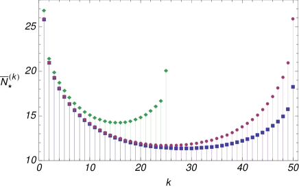
Figure 2: (Color online) Distribution of mean occupation numbers for the elements of a chain of two lengths. The (green) diamond-shaped points correspond to a chain of $n=25$ with $\bar{N}_{\rm A}=2\bar{N}_{\rm B}=10\bar{N}_{k}=100$. The (blue) square points are for $n=50$ with $\bar{N}_{\rm A}=2\bar{N}_{\rm B}=10\bar{N}_{k}=100$. Finally, the (violet) dots are for $n=50$ with $\bar{N}_{\rm A}=\bar{N}_{\rm B}=10\bar{N}_{k}=100$. The remaining parameters are $\Omega/\omega=1/2$, $\zeta/\omega=\zeta_{\rm A}/\omega=\zeta_{\rm B}/\omega=1/10$, $\hbar=1$. For all the three plots k =1,..,n.

As for the current, one finds

$$\mathcal{J} =-\frac{\zeta}{2}{\rm e}^{-\zeta t}\,{\rm Tr}(\mathbf{H}{\bf V}_{\!0})-\frac{\zeta}{2}{\rm e}^{-\zeta t}\langle\hat{x}\rangle_{0}\cdot{\bf H}\langle\hat{x}\rangle_{0}$$ (30)

$$+\hbar\omega\left(\frac{\zeta n}{2}+\zeta\sum_{k=1}^{n}\bar{N}_{k}\!+\!\zeta_{\rm A}\bar{N}_{\rm A}+\zeta_{\rm B}\bar{N}_{\rm B}\right){\rm e}^{-\zeta t}$$

with $\mathcal{J}_{\star}=0$. As the current is a linear function of the matrix $\lambda_{m}\lambda_{m}^{\dagger}$ [cf. Eq. (25)], in order to interpret each term of the above equation and their contribution to the total current at the steady state, we break the total current into the three parts. The first two are time independent and read

$$\mathcal{J}^{(l)}=\frac{\hbar}{2}{\rm Tr}\left[{\bf H}\,{\bf\Upsilon}^{(l)}\right]=\hbar\omega\zeta_{l}\bar{N}_{l}~{}~{}~{}~{}~{}~{}~{}(l={\rm A},{\rm B}).$$ (31)

The third one is

$$\mathcal{J}^{(k)} = \frac{\hbar}{2}{\rm Tr}\left[{\bf H}\,{\rm Re}{\bf\Upsilon}^{(k)}\right]-{\rm Tr}\left[{\bf H}{\bf V}\mathsf{J}\,{\rm Im}{\bf\Upsilon}^{(k)}\right]$$

$$= \hbar\omega\zeta(\bar{N}_{k}+1/2)\!-\!\zeta(\omega\,{\bf V}_{\!kk}+\Omega\,{\bf V}_{\!k-1k}+\Omega\,{\bf V}_{\!kk+1})\,.$$

For simplicity, we have omitted the explicit dependence on the initial conditions. The simple form attained in Eq. (31) is a consequence of Eq. (16), where the matrices ${\bf\Upsilon}^{({\rm A})}$ and ${\bf\Upsilon}^{({\rm B})}$ are purely real. At the steady state, using Eqs. (29) and (III), one finds

$$\mathcal{J}^{(1)}_{\star} =-\hbar\omega\zeta\left[\bar{N}^{(1)}_{\star}-\bar{N}_{1}\right]-\Omega\zeta\,{\bf V}_{\!\star 12},$$ (33)

$$\mathcal{J}^{(k)}_{\star} =-\hbar\omega\zeta\left[\bar{N}^{(k)}_{\star}-\bar{N}_{k}\right]-\Omega\zeta({\bf V}_{\!\star kk+1}+{\bf V}_{\!\star k-1k}),$$

$$\mathcal{J}^{(n)}_{\star} =-\hbar\omega\zeta\left[\bar{N}^{(n)}_{\star}-\bar{N}_{n}\right]-\Omega\zeta\,{\bf V}_{\!\star n-1n}.$$

The above currents for each reservoir in the chain at the stationary state are plotted in Fig. 3. It is possible to show, see the Appendix, that

$${\bf V}_{\!\star jj+1}=0,\,\,\,(j=1,...,n-1).$$ (34)

Thus the currents in Eq. (33) are given exclusively by the difference between the mean occupation number of the reservoirs $\bar{N}_{k}$, and the mean thermal photon number of each oscillator $\bar{N}^{(k)}_{\star}$. That is, the heat currents within the system can be understood as the difference between the amounts of energy stored in a given reservoirs and that in the respective oscillator. The fact that $\mathcal{J}_{\star}=0$ implies that all the internal currents ${\cal J}^{(k)}$ are constrained to sum up the (constant) value $-\left(\mathcal{J}^{({\rm A})}+\mathcal{J}^{({\rm B})}\right)$ independently on the length of the chain, which shows a clear violation of Fourier law of heat conduction. From Fig. 3 note that all the currents are negative showing also that the thermal energy stored in each oscillator, represented by $\bar{N}^{(k)}_{\star}$, is greater than the energy of its own reservoir, see Eq.(33).

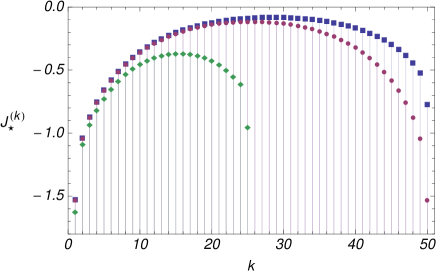
Figure 3: (Color online) Currents across the chain. The (green) diamond-shaped points correspond to a chain of $n=25$ with $\bar{N}_{\rm A}=2\bar{N}_{\rm B}=10\bar{N}_{k}=100$. The (blue) square points are for $n=50$ with $\bar{N}_{\rm A}=2\bar{N}_{\rm B}=10\bar{N}_{k}=100$. Finally, the (violet) dots are for $n=50$ with $\bar{N}_{\rm A}=\bar{N}_{\rm B}=10\bar{N}_{k}=100$. The remaining parameters are as in Fig. 2.

The general behavior of both quantities against the length of the chain can be seen from Fig. 4. For this range of $n$ (chain lengths) the local occupation number decreases with $n$ while the current does the opposite. As far as we could check numerically, for $n\gg 1$, both quantities become independent of the length of the chain. However, due to the lack of an analytical proof we cannot assure that this is really the case in the thermodynamic limit. Obviously, the relation Eq. (33) among these quantities is valid for any chain length. Furthermore, any oscillator in the bulk of the chain, i.e., any element identified by a label $k\sim n/2$, has the same occupation number of the reservoir attached to it. This is due to the fact that, by Eq. (20), ${\bf O}_{kj}\approx\sqrt{2/n}\sin(j\pi/2)$ and $\bar{N}^{(k)}_{\star}=\bar{N}_{k}$. Moreover, the individual currents, i.e., the currents due to the local standard thermal baths, are null according to Eq. (33). This implies that in this limit the local baths play no major role in the thermalization of the bulk oscillators. In this respect, our results share some similarity with the classical approach of the problem, where a chain of harmonic oscillators is attached to just two thermal baths at its ends. In fact, in the work by Reider et al. rieder , the bulk oscillators attains a constant temperature as in our case when the limit $n\gg 1$ is considered.

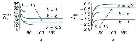
Figure 4: (Color online) Mean value of energy (left) and currents (right) for the fixed-position oscillators [the first $(k=1)$ and the 10${}^{\text{th}}$ ($k=10$ )], the midpoint (bulk) $k=n/2$, and the last oscillator $k=n$. We consider $\bar{N}_{\rm A}=2\bar{N}_{\rm B}=10\bar{N}_{k}=100$; the remaining parameters are the same as in Fig. 2.

IV Application to paradigmatic cases

In this section we use the formalism and results illustrated so far to analyze the transport of heat in a few paradigmatic examples, all encompassed by the general treatment of the problem provided above. In particular, we want to study the effects caused by the presence of end-chain all-diffusive reservoirs, something not yet explored in this context before. To this end, we now consider different variations on the basic setup described on Fig. 1. For example, we vary the distribution of reservoirs, the coupling mechanism among the oscillators and include dephasing.

IV.1 Case I: Ordinary Baths

In order to establish a benchmark to evaluate the role played by the diffusive baths, we start the analysis by taking $\zeta_{\rm A}=\zeta_{\rm B}=0$ in (15). The corresponding steady-state CM is as in Eq. (21) with

$${\boldsymbol{D}}=\hbar\zeta\,{\rm Diag}({\bar{N}_{1},...,\bar{N}_{n}}),$$ (35)

while the steady-state energy and the current are given by Eq. (28) and Eq. (30), respectively. In order to remain as close as possible to the system discussed in the previous section, we take $T_{1}>T_{k}>T_{n}$ for $1<k<n$. As all reservoirs are of the ordinary type, the approximation in Eq. (15) does not hold for the end-chain baths. However, as one can see from Fig. 5, the same pattern for the mean excitation number displayed in Fig. 2 is found. In Fig. 6, we then plot the currents, given in Eq. (33), generated by the attachment to the reservoirs with temperatures $T_{k}$, $k=2,...,n-1$. They are all negative, as in Fig. 3, and sum up to

$$\sum_{k=2}^{n-1}\mathcal{J}^{(k)}_{\star}=-(\mathcal{J}^{(1)}_{\star}+\mathcal{J}^{(n)}_{\star})<0.$$ (36)

However, the actual value of the sum of the currents depends on the number of oscillators since $\mathcal{J}^{(1)}_{\star}$ and $\mathcal{J}^{(n)}_{\star}$ depends on the length of the system. Again, the individual currents are the difference between the energy stored in each oscillator and the mean energy occupation of the respective reservoir. As the number of oscillators in the chain increases, the current and mean energy behave very much like those in Fig. 4.

At this point, one might wonder about the reason for the negativity of the internal currents. Actually, it turns out that this is a simple consequence of the structure of Eq. (33) when Eq. (34) is taken into account: numerical explorations shows that the oscillators attached to the highest temperature reservoirs will have $\bar{N}_{k}{-}\bar{N}^{(k)}_{\star}>0$, while the other oscillators will not as their occupation number will also be determined by their own lower-temperature reservoir and the contributions coming from the higher-temperature ones.

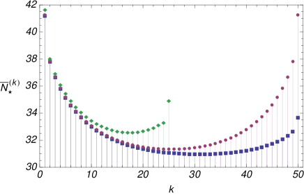
Figure 5: (Color online) Distribution of mean occupation numbers for the elements of a chain without the diffusive reservoirs. Diamonds (green): chain with $n=25$ oscillators and temperatures of the baths given in terms of $\bar{N}_{1}=2\bar{N}_{n}=100$ and $\bar{N}_{k}=30$; Squares (blue): chain with $n=50$ oscillators and $\bar{N}_{1}=2\bar{N}_{n}=100$ and $\bar{N}_{k}=30$; Circles (violet): $n=50$ and $\bar{N}_{1}=\bar{N}_{n}=100$ and $\bar{N}_{k}=30$. The remaining parameters are the same as in Fig. 2 except for $\zeta_{\rm A}$ and $\zeta_{\rm B}$, which taken to be zero and in all cases $k=2,...,n-1$.

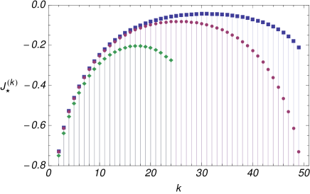
Figure 6: (Color online) Currents across the chain without the diffusive reservoirs. The color-symbol code is the same as in Fig. 5, although we have taken $k=2,...,n-1$, i.e., we have excluded the positive currents from the first and last reservoir.

In Fig. 7, we plot the results valid for a different configuration, where one internal reservoir has the highest temperature. Notwithstanding the differences with respect to the patterns shown in Figs. 5 and 6, the currents and energy of this configuration follow the same chain-length dependence discussed above.

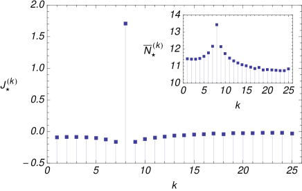
Figure 7: (Color online) Currents across a chain of $n=25$ oscillators with $\bar{N}_{8}=30$ and $\bar{N}_{k}=10,\forall k\neq 8$. The remaining parameters are the same as in Fig. 2. Inset: Mean occupation number of the oscillators in the chain.

IV.2 Case II: All-diffusive dynamics

Let us consider now a chain of oscillators connected only to the all-diffusive reservoirs $\rm A$ and $\rm B$. When $\zeta_{k}=0$ for $k=1,\dots,n$ the resulting dynamics is not stable (cf. Appendix). However, the evolution of the system can be deduced from Eq. (19) by taking $\zeta\to 0$ to give

$$\!\!\!\!\!\!\!\!{\bf V}(t) ={\rm e}^{\mathsf{J}{\bf H}t}\,{\bf V}\!_{0}\,{\rm e}^{-{\bf H}\mathsf{J}t}$$ (37)

$$+{\bf O}\!\oplus\!{\bf O}\left(\!\!\begin{array}[]{rr}{\bf O}{\boldsymbol{D}}{\bf O}\circ{{\rm Re}\bf L}_{0}&-{\bf O}{\boldsymbol{D}}{\bf O}\circ{{\rm Im}\bf L}_{0}\\ {\bf O}{\boldsymbol{D}}{\bf O}\circ{{\rm Im}\bf L}_{0}&{\bf O}{\boldsymbol{D}}{\bf O}\circ{{\rm Re}\bf L}_{0}\end{array}\!\!\right){\bf O}\!\oplus\!{\bf O},$$

with $({{\bf L}_{0}})_{jk}=\lim_{\zeta\to 0}{\bf L}_{jk}=i({\rm e}^{-i(\nu_{j}-\nu_{k})t}-1)/({\nu_{j}-\nu_{k}})$. The diagonal elements of ${{\bf L}_{0}}$ are obtained taking the limit $\nu_{j}\to\nu_{k}$ and are given by $({{\bf L}_{0}})_{kk}=t,\forall k$. Note that the ordering of the two limits above does not commute. As in the case of Eq.(21), the matrix elements $({{{\rm Im}\bf L}_{0}})_{kk}=0,\forall k$. Consequently, the reduced CM of each oscillator is diagonal meaning that it is a thermal state for any time instant.

In Fig. 8, we show the mean occupation number of each oscillator, $\bar{N}^{(k)}={\bf V}(t)_{kk}/\hbar-1/2$, at some instants of time for the evolution in Eq. (37) and an initial vacuum state. The process of excitation of the elements of the chain starts from its ends to then progressively move towards its center. The mean occupation number of the oscillators increases on average linearly in time, i.e., they oscillate by the effect of the orthogonal matrices $\bf O$ around the linear rate given by $[{{\bf L}_{0}}]_{kk}$ [cf. Eq. (37)].

As an interesting remark, we observe that the distribution corresponding to the case of $t=20$ displays oscillators having occupation numbers larger than those of the oscillators in touch with the all-diffusive reservoirs. This is an effect of the competition between linear time increase of $\bar{N}_{k}$ and the oscillatory behavior induced by the actual absence of a steady state.

The total current for this system is obtained as

$${\mathcal{J}}_{0}:=\lim_{\zeta\to 0}\mathcal{J}=\omega\left[\zeta_{\rm A}\bar{N}_{\rm A}+\zeta_{\rm B}\bar{N}_{\rm B}\right],$$ (38)

and is thus a constant and that helps us in determining the mean energy of the system

$$\lim_{\zeta\to 0}\langle\hat{H}\rangle_{t}=\tfrac{1}{2}{\rm Tr}(\mathbf{H}{\bf V}_{\!0})+{\mathcal{J}}_{0}\,t.$$ (39)

The indefinite growth of energy supplied by the current can be seen as a signature of instability of the system. In this context, the relative temperature of the two reservoirs is irrelevant since both contributes additively for the energy [Eq. (39)] and for the current [Eq. (38)].

Figure 8: (Color online) Distribution of mean occupation numbers for the elements of a chain of $n=25$ oscillators attached only to two end-chain diffusive reservoirs. We sample the dynamics at the instants of time $t=1,10,20,30$. The chain is initially prepared in its vacuum state. We have taken $\zeta_{\rm A,B}=1/10$ and $\bar{N}_{\rm A}=2\bar{N}_{\rm B}=100$. As for the other parameters of the system, we have $\Omega/\omega=1/2$ and $\hbar=1$.

IV.3 Case III: Balanced competition of environmental effects

A standard thermal reservoir, as those distributed across the chain in Fig. 1, exchanges energy with the system in two distinct ways: diffusion, described by the matrix $\bf D$ in Eq. (7), which is responsible of the enhancement of energy; and dissipation, described by $\bf\Gamma$, which extracts energy from the system. The balanced competition of these two effects drives the system to equilibrium at the steady state.

So far, the ordinary reservoirs and the all-diffusive have not been treated on equal footing, and it will be interesting to understand the behavior of a chain when a balanced competition of environmental mechanisms is considered. To this end, let us consider the system depicted in Fig. 1 with $\zeta_{m}=0$ for $1<m<n$, i.e., while the reservoirs of the bulk chain are detached, those at the end of it (having temperatures $T_{1}$, $T_{n}$, $T_{\rm A}$, and $T_{\rm B}$) are still operative. In this case, the matrices (7) are given by

$${\bf\Gamma}={\boldsymbol{G}}\oplus{\boldsymbol{G}}+{\mathsf{J}}({\boldsymbol{H}}\!\oplus\!{\boldsymbol{H}}),\,\,\,{\bf D}={\boldsymbol{D}}\!\oplus\!{\boldsymbol{D}},$$ (40)

with ${\boldsymbol{G}}=-\tfrac{1}{2}{\rm Diag}(\zeta_{1},0,...,0,\zeta_{n})$ and

$${\boldsymbol{D}}=\hbar\zeta\,{\rm Diag}(\bar{N}_{1}+\tfrac{1}{2}+\tfrac{\zeta_{\rm A}}{\zeta}\bar{N}_{\rm A},0,...,0,\bar{N}_{n}+\tfrac{1}{2}+\tfrac{\zeta_{\rm B}}{\zeta}\bar{N}_{\rm B}).$$

The stability of this system is independent of the diffusive reservoirs since they did not contribute to ${\bf\Gamma}$ in Eq. (40). Furthermore, the action of the all-diffusive reservoirs is only to enhance the mean occupation number of the standard ones, that is, the solution to this problem is equivalent to take a chain with only two end-system standard reservoirs with mean occupation numbers $\tilde{N}_{1}=\bar{N}_{1}+({\zeta_{\rm A}}/{\zeta})\bar{N}_{\rm A}$ and $\tilde{N}_{2}=\bar{N}_{2}+({\zeta_{\rm B}}/{\zeta})\bar{N}_{\rm B}$. The methods employed in Ref. assadian , which addressed the problem embodied by Eq. (40) with $\zeta_{\rm A}=\zeta_{\rm B}=0$, will be useful to find a solution to this case. At the steady state attained by Eq. (40), the sum of all currents is null (as expected) while the mean occupation number for each oscillator is given by the expressions

$$\bar{N}^{(1)}_{\star} =\tfrac{1}{2}(\tilde{N}_{1}+\tilde{N}_{n})+\frac{\zeta^{2}(\tilde{N}_{1}-\tilde{N}_{n})}{8\Omega^{2}+2\zeta^{2}},$$ (41)

$$\bar{N}^{(k)}_{\star} =\tfrac{1}{2}(\tilde{N}_{1}+\tilde{N}_{n})~{}~{}(1<k<n),$$

$$\bar{N}^{(n)}_{\star} =\tfrac{1}{2}(\tilde{N}_{1}+\tilde{N}_{n})-\frac{\zeta^{2}(\tilde{N}_{1}-\tilde{N}_{n})}{8\Omega^{2}+2\zeta^{2}}.$$

All the internal oscillators have the same occupation number, as in Ref. assadian . The mean energy at the steady state can be evaluated from Eq. (27)

$$\langle\hat{H}\rangle_{\star}=\hbar\omega\sum_{k=1}^{n}(\bar{N}^{(k)}_{\star}+\tfrac{1}{2})=n\hbar\omega\left(\frac{\tilde{N}_{1}+\tilde{N}_{n}}{2}+\frac{1}{2}\right).$$ (42)

The currents through the two oscillators are given by Eq. (III), i.e., $\mathcal{J}^{(k)}_{\star}=-\hbar\omega\zeta(\bar{N}^{(k)}_{\star}-\tilde{N}_{k})$ with $k=1,n$ and are equal to

$$\mathcal{J}^{(1)}_{\star}=-\mathcal{J}^{(n)}_{\star}=\frac{2\hbar\omega\Omega^{2}\zeta(\tilde{N}_{1}-\tilde{N}_{n})}{4\Omega^{2}+\zeta^{2}}.$$ (43)

This perfect balance implies that the currents at the stationary state for the two standard reservoirs are constrained to sum up $\mathcal{J}^{(\rm A)}+\mathcal{J}^{(\rm B)}$ which is the sum of the currents due to the all-diffusive ones. This is analogous to what we have witnessed in Sec. II. Since $\tilde{N}_{k}=[\exp(\hbar\beta_{k}\omega)-1]^{-1}$, where $\beta_{k}$ is the inverse temperature, one can see that, in the classical limit $\hbar\to 0$, the current [Eq. (43)] and the temperature of each reservoir in the bulk [Eq. (41)] behave as in the classical case rieder . That means that the currents are proportional to the temperature difference and the bulk oscillators thermalize at the mean value temperature of the reservoirs.

IV.4 Case IV: Dephasing dynamics

In Ref. assadian , Assadian et al. considered a chain of oscillators attached to two standard thermal reservoirs at the ends, which is the same configuration described in Sec. IV.3 but with $\zeta_{\rm A}=\zeta_{\rm B}=0$. Under these restrictions, the results in Eq. (42) and (43) remain valid and can be extracted from their work.

Besides this example, they consider also the presence of $n$ purely dephasing reservoirs, each one attached to each oscillator of the chain. The contribution of the dephasing mechanisms to the dynamics is modelled adding the following Lindblad operators to the master equation regulating the dynamics of the system

$$\hat{L}_{k}=\hbar\sqrt{\gamma}\,\hat{a}_{k}^{\dagger}\hat{a}_{k},\,\,\,k=1,...,n.$$ (44)

The special form of these reservoirs is such that they do not introduce new currents in the system. This can be verified by calculating the individual currents to find that $\mathcal{J}_{k}=0,\forall k$. On the other hand, their presence drastically changes the behavior of the mean occupation value of each oscillator . As it can be seen from Eq. (29), these are now given by assadian

$$\bar{N}^{(1)}_{\star} =\tfrac{1}{2}(\bar{N}_{1}+\bar{N}_{n})+\frac{[\zeta^{2}+(n-1)\gamma\zeta](\bar{N}_{1}-\bar{N}_{n})}{8\Omega^{2}+2\zeta^{2}+2(n-1)\gamma\zeta},$$ (45)

$$\bar{N}^{(k)}_{\star} =\tfrac{1}{2}(\bar{N}_{1}+\bar{N}_{n})+\frac{(n-2k+1)\gamma\zeta(\bar{N}_{1}-\bar{N}_{n})}{8\Omega^{2}+2\zeta^{2}+2(n-1)\gamma\zeta},$$

$$\bar{N}^{(n)}_{\star} =\tfrac{1}{2}(\bar{N}_{1}+\bar{N}_{n})-\frac{[\zeta^{2}+(n-1)\gamma\zeta](\bar{N}_{1}-\bar{N}_{n})}{8\Omega^{2}+2\zeta^{2}+2(n-1)\gamma\zeta}$$

for $1<k<n-1$. Note that if the temperature of standard end-chain reservoirs are equal, $\bar{N}_{1}=\bar{N}_{n}=\bar{N}$, all the oscillators thermalize with the standard reservoirs having the same mean occupation number $\bar{N}$. The behavior of the mean occupation number is plotted in Fig. 9.

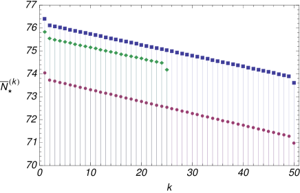
Figure 9: (Color online) Distribution of mean occupation numbers for the elements of a chain connected to two ordinary end-chain reservoirs and $n$ dephasing reservoirs. Diamonds (green): chain with $n=25$ oscillators and bath mean occupation numbers $\bar{N}_{1}=2\bar{N}_{n}=100$. Squares (blue): chain with $n=50$ oscillators and $\bar{N}_{1}=2\bar{N}_{n}=100$. Circles (violet): $n=50$ and $\bar{N}_{1}=4\bar{N}_{n}/3=100$. All other parameters are as in Fig. 2.

As already commented, the dephasing reservoirs do not contribute to the currents. At the stationary state, we have

$$\mathcal{J}^{(n)}_{\star}=-\mathcal{J}^{(1)}_{\star}=\frac{2\hbar\omega\Omega^{2}\zeta(\bar{N}_{1}-\bar{N}_{n})}{4\Omega^{2}+\zeta^{2}+(n-1)\gamma\zeta}.$$ (46)

This result is remarkable, as it shows that for $4\Omega^{2}+\zeta^{2}\ll n\gamma\zeta$, which is trivially satisfied for a large enough chain, a Fourier-like dependence on the size of the system is recovered assadian . The classical version of the same problem has been studied in Ref. landi .

We now describe the modifications induced by the dephasing reservoirs when they are attached, one by one, to the system. The Lindblad operator in Eq. (44) can be rewritten as (see also the Appendix)

$$\hat{L}_{m}=\tfrac{1}{2}\hat{x}\cdot{\Delta}_{m}\hat{x}+\lambda_{m}\cdot\mathsf{J}\hat{x}+\mu_{m},$$ (47)

with the $2n\times 2n$ real matrix

$$[{\bf\Delta}_{m}]_{jk}=\sqrt{\gamma_{m}}(\delta_{jm}\delta_{mk}+\delta_{j+n\,m}\delta_{m\,k+n}).$$ (48)

Without dephasing reservoirs ($\gamma_{m}=0,\forall m$), the currents in the system are the ones described by (43) with the substitutions $\tilde{N}_{1}\to\bar{N}_{1}$ and $\tilde{N}_{n}\to\bar{N}_{n}$. Following the prescriptions in the Appendix, we solve numerically the system with $\gamma_{1}=\gamma$ and $\gamma_{k}=0\,\forall k\neq 1$, $n\leq k\leq 1$ and calculate the current as function of the number of oscillators $n$. Adding progressively more dephasing reservoirs until $\gamma_{m}=\gamma,\forall m$ [in this situation the current is given by Eq. (46)] and calculating the current allows us to show in Fig. 10 the smooth transition from the situation described by Eq. (43) to that associated to Eq. (46).

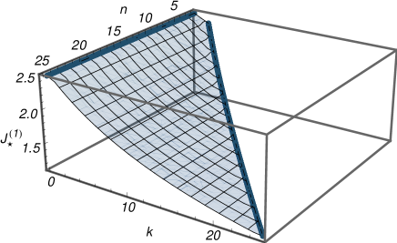
Figure 10: (Color online) Current across the chain with two ordinary end-chain reservoirs, plotted as a function of the number of oscillators $n$ and the number of dephasing reservoirs $k$. We highlight the curves describing the extreme cases $k=0$ and $k=n$, which are the functions reported, respectively, in Eq. (43) with $\tilde{N}_{1}=2\tilde{N}_{2}=100$ and in Eq. (46) with $\bar{N}_{1}=2\bar{N}_{2}=100$. The dephasing coupling is $\gamma/\omega=0.5$ while the remaining parameters are the same as in Fig. 2.

IV.5 Case V: Disorder Effect

Classically, size-dependent currents in chains of oscillators arise under the presence of anharmonicity or disorder dhar , which can be realized in various ways. One can, for example, introduce different frequencies and/or couplings across the chain. For the sake of definiteness, we consider the system of Fig. 1, now ruled by the Hamiltonian

$$\hat{H}=\hbar\omega\sum_{j=1}^{n}\hat{a}_{j}^{\dagger}\hat{a}_{j}+2\hbar\sum_{j=1}^{n-1}\Omega_{j}(\hat{a}_{j}^{\dagger}\hat{a}_{j+1}+\hat{a}_{j+1}^{\dagger}\hat{a}_{j}).$$ (49)

The structure of Eq. (21) remains the same with $\bf O$ being replaced by the matrix that diagonalizes the adjacency matrix

$${\boldsymbol{H}}_{\!jk}=\omega\,\delta_{jk}+\Omega_{j}\,(\delta_{j\,k+1}+\delta_{j\,k-1})$$ (50)

and $\nu_{k}$ (which appears in the definition for ${\bf L}_{\star}$) being its eigenvalues and both can be calculated numerically for a given set of couplings $\{\Omega_{j}\}_{1\leq j\leq n}$. To introduce disorder, we arbitrary choose a set of coupling constants $\Omega_{j}$ with magnitudes similar to what has been considered so far.

In Figs. 11 and 12, respectively, we plot the mean occupation number and the current for a set of distinct coupling constants. Structurally speaking, the behavior of the system does not change with the introduction of disorder. This can be seen when comparing these figures, respectively, with Fig. 2 and Fig. 3. Observe the similarities on the profile of the curves, the first, and last oscillators and, mainly, the behavior of the bulk. Furthermore, for the quantities shown in Figs. 11 and 12, we also have analyzed different sets of inhomogeneous constant couplings $\{\Omega_{j}\}$. In the units of the paper, each $\Omega_{j}$ is bounded by $(0,1]$ in our simulations in order to keep a fair comparison of the results. From these simulations, results obtained using different sets differ, but the general trends shown in those plots are preserved, especially the behavior of the bulk oscillators.

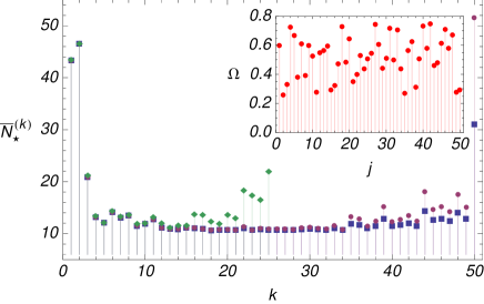
Figure 11: (Color online) Distribution of mean occupation numbers for the elements of a chain with distinct coupling constants. Inset: Set of coupling constants used in the simulation. The remaining parameters are as Fig. 2.

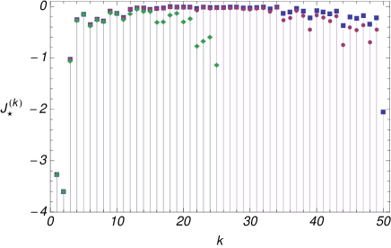
Figure 12: (Color online) Currents across the chain for the same situation depicted in Fig. 11.

It is also interesting to see what happens with the individual currents and occupation numbers near the thermodynamical limit. These are plotted in Fig. 13. As before, currents and mean occupation numbers for the oscillators in the bulk become independent on the length for long-enough chains. However, it is interesting to remark that the last oscillator is strongly influenced by the disorder while the behavior of the remaining oscillators is essentially the same as in the case of Fig. 4.

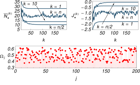
Figure 13: (Color online) Mean value of energy (left) and currents (right) for fixed position oscillators [the first $(k=1)$ and the 10${}^{\text{th}}$ $(k=10)$], the midpoint (bulk) $k=n/2$, and the last oscillator $k=n$ for a chain with distinct constant couplings. Bottom panel: Set of coupling constants used in the simulation. We consider $\bar{N}_{\rm A}=2\bar{N}_{\rm B}=10\bar{N}_{k}=100$. The remaining parameters are the same as in Fig. 2.

IV.6 Case VI: Spring-mass coupling

Until now, we have worked in the regime of the rotating-wave approximation (RWA), which enables the explicit analytical form of the CM of the chain [cf. Eq.(19)]. This contrasts significantly with any classical approach to the transmission of heat across a harmonic chain, which is in general performed assuming the standard spring-mass coupling (SMC) rieder ; dhar ; landi . In this subsection we will thus briefly address the case of an SMC-like coupling to make a more faithful comparison with the classical case.

The Hamiltonian of a chain of $n$ oscillators coupled by the standard SMC coupling has the adjacency matrix $\mathbf{H}^{\prime}={\boldsymbol{H}}^{\prime}\oplus\omega\mathsf{I}_{n}$, where

$${\boldsymbol{H}}^{\prime}_{\!jk}=\,(\omega+\kappa)\,\delta_{jk}-\tfrac{\kappa}{2}(\delta_{j\,k\pm 1}+\delta_{j1}\delta_{1k}+\delta_{jn}\delta_{nk}).$$ (51)

As this matrix is almost of the Toeplitz form, a procedure similar to the one used in the Appendix can be used to find the covariance matrix of the system, which is given by

$${\bf V}={\bf O}_{{\bf\Gamma}^{\prime}}^{-1}\left[{\bf O}_{{\bf\Gamma}^{\prime}}{\bf D}{\bf O}_{{\bf\Gamma}^{\prime}}^{\top}\circ{{\bf L}^{\prime}_{\star}}\right]{\bf O}_{{\bf\Gamma}^{\prime}}^{-\top}.$$ (52)

Here $[{\bf L}^{\prime}_{\star}]_{jk}=-1/(\nu_{j}^{\prime}-\nu_{k}^{\prime})$ with

$$\nu^{\prime}_{k}=\sqrt{\omega(\omega+\kappa)-\omega\kappa\cos\left[(m-1)\pi/n\right]},$$ (53)

and ${\bf O}_{{\bf\Gamma}^{\prime}}$ defined by

$$\!\!{\bf O}_{{\bf\Gamma}^{\prime}}{\bf\Gamma}^{\prime}{\bf O}_{{\bf\Gamma}^{\prime}}^{-1}=-\frac{\zeta}{2}\mathsf{I}_{2n}+{\rm Diag}(i\nu^{\prime}_{1},...,i\nu^{\prime}_{n},-i\nu^{\prime}_{1},...,-i\nu^{\prime}_{n}).$$ (54)

We can now calculate the mean occupation number and the current for each oscillator, whose behavior is shown in Fig. 14 and Fig 15, respectively.

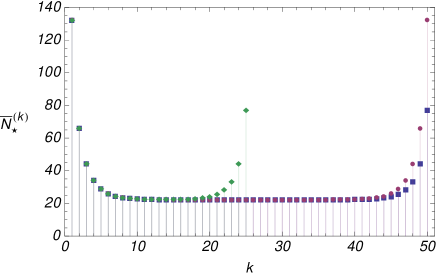
Figure 14: (Color online) Distribution of mean occupation numbers for the elements of a chain of two lengths for the SMC Hamiltonian. Diamonds (green): chain of $n=25$ with $\bar{N}_{\rm A}=2\bar{N}_{\rm B}=10\bar{N}_{k}=100$; Squares (blue): chain of $n=50$ with $\bar{N}_{\rm A}=2\bar{N}_{\rm B}=10\bar{N}_{k}=100$; Circles (violet): $n=50$ with $\bar{N}_{\rm A}=\bar{N}_{\rm B}=10\bar{N}_{k}=100$. The remaining parameters are $\kappa/\omega=1/2$, $\zeta/\omega=\zeta_{\rm A}/\omega=\zeta_{\rm B}/\omega=1/10$, and $\hbar=1$.

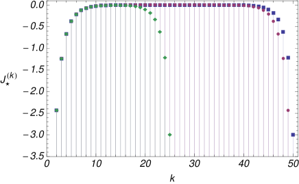
Figure 15: (Color online) Currents across the chain for the SMC Hamiltonian. We used the same parameters as in Fig. 14.

As one can see, the results for the SMC case are structurally similar to those found in the RWA. Such similarities extend also to the situations where either the diffusive baths are not considered or the distribution of coupling constants across the chain is not uniform.

V Conclusions

We have investigated heat transport in quantum harmonic chains connected to different types of heat baths. We have obtained the exact expression for the currents across the system highlighting the crucial role played by the properties of the environment. Such detailed analysis was instrumental to the study of a few paradigmatic configurations. In particular, just like in Ref. assadian , we have found that the Fourier law is not predicted by the models considered here unless dephasing is included, destroying the ballistic behavior. This is akin to a substrate external potential in the classical version of the problem addressed here. In our findings, Fourier law is still not observed in the presence of disorder as long as the coupling with the bath is weak, allowing a description using a Markovian master equations, as addressed in this manuscript. Our results are consistent with those known for unidimensional classical harmonic chains and shed new light on the interplay between transport properties of spatially extended quantum media and the nature of the environmental systems interacting with it.

Appendix

In this Appendix we provide additional details on the mathematical approach to the problems addressed in the main body of the paper.

Currents and energy for a quadratic system

Here we address the derivation of the expressions for the currents and mean energy for a system evolving according to Eq. (4) when a quadratic Hamiltonian as the one in Eq. (5) and quadratic Lindblad operators are considered. Specifically, we assume the form

$$\hat{L}_{m}=\tfrac{1}{2}\hat{x}\cdot{\Delta}_{m}\hat{x}+\lambda_{m}\cdot\mathsf{J}\hat{x}+\mu_{m},$$ (A-1)

where $\Delta_{m}=\Delta_{m}^{\top}$ is a $2n\times 2n$ real matrix. Taking the derivative of $\langle\hat{x}\rangle_{t}$ and $\bf V$ defined in Eq. (3), using the master equation (4), and recalling the commutation relation $[\hat{x}_{j},\hat{x}_{k}]=i\hbar\,\mathsf{J}_{jk}$, we get the dynamical equations

$$\frac{d\langle\hat{x}\rangle_{t}}{dt}=\xi-\eta+{\bf\tilde{\Gamma}}\langle\hat{x}\rangle_{t},~{}~{}\frac{d\mathbf{V}}{dt}={\tilde{\bf\Gamma}}\mathbf{V}+\mathbf{V}{\tilde{\bf\Gamma}}^{\top}+{\bf D}+{\bf\Delta}_{\!\bf V},$$ (A-2)

where

$${\bf\Delta}_{\!\bf V}=\hbar\sum_{m}\mathsf{J}{\Delta}_{m}{\bf V}\,{\Delta}_{m}\mathsf{J}^{\top},~{}~{}\tilde{\bf\Gamma}={\bf\Gamma}+\tfrac{\hbar}{2}\sum_{m}(\mathsf{J}\Delta_{m})^{2}.$$ (A-3)

Both $\bf\Gamma$ and $\bf D$ are defined in Eq. (7). By inserting Eq. (5) and Eq. (A-1) into the definition of the individual ${\mathcal{J}}_{m}$’s in Eq. (24), we get

$$\mathcal{J}_{m} = \tfrac{\hbar}{2}{\rm Tr}\left[{\bf H}{\rm Re}\left(\lambda_{m}\lambda_{m}^{\dagger}\right)-{\bf H}\mathsf{J}{\Delta}_{m}{\bf V}{\Delta}_{m}\mathsf{J}\right]$$ (A-4)

$$+ \tfrac{\hbar}{2}{\rm Tr}\left[{\bf H}(\mathsf{J}\Delta_{m})^{2}\left({\bf V}+\langle\hat{x}\rangle_{t}\langle\hat{x}\rangle_{t}^{\top}\right)\right]$$

$$- {\rm Tr}\left[{\bf H}\,{\rm Im}\left(\lambda_{m}\lambda_{m}^{\dagger}\right)\mathsf{J}\left({\bf V}+\langle\hat{x}\rangle_{t}\langle\hat{x}\rangle_{t}^{\top}\right)\right]$$

$$+ \mathsf{J}\xi\cdot\left[{\rm Im}\left(\lambda_{m}\lambda_{m}^{\dagger}\right)\mathsf{J}-\hbar\mathsf{J}{\Delta}_{m}{\bf V}\,{\Delta}_{m}\mathsf{J}\right]\langle\hat{x}\rangle_{t}$$

$$+ {\rm Im}(\mu_{m}^{\ast}\lambda{{}_{m}})\cdot(\mathsf{J}\xi-\mathbf{H}\langle\hat{x}\rangle_{t}).$$

Summing over all Lindblad operators, see Eq. (24), the total current has the following form

$$\!\!\!\!\!\!\!\!\!\mathcal{J}= \,\frac{1}{2}{\rm Tr}\left[{\bf H}(\,{\bf D}+{\bf\Delta}_{\!\bf V})\right]+{\rm Tr}\left[{\bf H}\,{\tilde{\bf\Gamma}}\left({\bf V}+\langle\hat{x}\rangle_{t}\langle\hat{x}\rangle_{t}^{\top}\right)\right]$$ (A-5)

$$+\,(\xi-\eta)\cdot\mathbf{H}\langle\hat{x}\rangle_{t}-\mathsf{J}\xi\cdot\tilde{\bf\Gamma}\langle\hat{x}\rangle_{t},$$

which is zero for a possible steady state, i.e., the solution of (A-2) with $\partial_{t}{\langle\hat{x}\rangle_{t}}=\partial_{t}{\mathbf{V}}=0$. The internal energy of the system is easily worked out as $\langle\hat{H}\rangle_{t}={\rm Tr}(\hat{H}\hat{\rho})$. We get

$$\langle\hat{H}\rangle_{t}=\tfrac{1}{2}{\rm Tr}\left[{\bf H}\,{\bf V}(t)+{\bf H}\,\langle\hat{x}\rangle_{t}\langle\hat{x}\rangle_{t}^{\top}\right]+\xi\cdot\mathsf{J}\langle\hat{x}\rangle_{t}+H_{0}.$$ (A-6)

Taking the derivative of this equation and rearranging the expressions one also finds Eq. (A-5).

On the stability of the dynamical system

Here we analyze the dynamical stability of the system discussed in Sec. II.

The matrix $\boldsymbol{H}$ given by Eqs. (12) and appearing in (17) is tridiagonal and symmetric Toeplitz, and can thus be diagonalized by a simple (symmetric) orthogonal transformation kulkarni as ${\bf O\boldsymbol{H}\bf O^{\top}}={\rm Diag}(\nu_{1},...,\nu_{n})$, where

$${\bf O}_{kl}=\sqrt{\tfrac{2}{n+1}}\,\sin\tfrac{kl\,\pi}{n+1},~{}~{}\nu_{m}=\omega+2\Omega\cos\tfrac{m\,\pi}{n+1}.$$ (A-7)

The matrix that diagonalizes $\bf\Gamma$ in (17) can then be constructed as ${\bf O}_{\bf\Gamma}=({\bf O}\!\oplus\!{\bf O}){\bf U}$ with

$${\bf U}=\frac{1}{\sqrt{2}}\left(\begin{array}[]{rl}-i\mathsf{I}_{n}&\mathsf{I}_{n}\\ i\mathsf{I}_{n}&\mathsf{I}_{n}\end{array}\right),$$ (A-8)

which gives us

$${\bf O}_{\bf\Gamma}{\bf\Gamma}{\bf O}_{\bf\Gamma}^{\dagger}=-\tfrac{\zeta}{2}\mathsf{I}_{2n}-i\,{\rm Diag}(\nu_{1},...,\nu_{n},-\nu_{1},...,-\nu_{n}).$$ (A-9)

As the spectrum in Eq. (A-9) has positive real part, $\bf\Gamma$ is stable. Moreover, in light of the fact that $\mathbf{D}$ in Eq. (17) is a positive definite matrix, the system allows for a steady state, whose moments are given by (9).

Details on the calculation of Eq. (18)

By integrating the expression for ${\bf I}$ by parts, we get

$$i[{\bf I},{\boldsymbol{H}}]-\zeta{\bf I}={\rm e}^{-i{\boldsymbol{H}}t}{\boldsymbol{D}}{\rm e}^{i{\boldsymbol{H}}t}{\rm e}^{-\zeta t}-{\boldsymbol{D}}.$$ (A-10)

By diagonalizing ${\boldsymbol{H}}$ with the help of Eq. (A-7) and introducing the matrices $\tilde{\bf I}={\bf O}{\bf I}{\bf O}$, $\tilde{\boldsymbol{D}}={\bf O}{\boldsymbol{D}}{\bf O}$, and $\bf L$ given in Eq. (20), we find that $\tilde{\bf I}_{jk}=\tilde{\boldsymbol{D}}_{\!jk}{\bf L}_{jk}=(\tilde{\boldsymbol{D}}\circ{\bf L})_{jk}$. Starting from this, one can straightforwardly show that

$${\bf I}={\bf O}\left[{\bf O}{\boldsymbol{D}}{\bf O}\circ{\bf L}\right]{\bf O}.$$ (A-11)

In turn, the dynamical solution in Eq. (18) can be obtained by using this result and noticing that

$${\bf U}^{\dagger}\,({\bf I}\oplus{\bf I}^{\ast})\,{\bf U}=\left(\begin{array}[]{cr}{\rm Re}{\bf I}&-{\rm Im}{\bf I}\\ {\rm Im}{\bf I}&{\rm Re}{\bf I}\end{array}\right).$$ (A-12)

Structural Properties of the CM

We now analyze some structural details of the blocks of the CM in Eq. (21), which with the help of (A-11) becomes

$${\bf V}_{\!\star}=\frac{\hbar}{2}\mathsf{I}_{2n}\,+\begin{pmatrix}{\rm Re}{\bf I}_{\star}&-{\rm Im}{\bf I}_{\star}\\ {\rm Im}{\bf I}_{\star}&{\rm Re}{\bf I}_{\star}\end{pmatrix},$$ (A-13)

where ${\bf I}_{\star}={\lim_{t\to\infty}}{\bf I}$ is a $n\times n$ Hermitian matrix. Actually, we want to demonstrate that ${\bf I}_{\star}$ satisfies

$${{\rm Re}{\bf I}_{\star}}_{jk}=0\,\,\,\text{if}\,\,\,j+k\,\,\,\text{ is odd},$$ (A-14)

$${{\rm Im}{\bf I}_{\star}}_{jk}=0\,\,\,\text{if}\,\,\,j+k\,\,\,\text{ is even},$$

which also proves the assertion on Eq. (34).

We start by defining the function

$$\Phi_{jk}(l,m,r):={\bf O}_{jl}{\bf O}_{lm}{\boldsymbol{D}}^{(m)}{\bf O}_{mr}{\bf O}_{rk}{\bf L_{\star}}_{lr}$$ (A-15)

with ${\boldsymbol{D}}^{(m)}={\boldsymbol{D}}_{mm}$, in such a way that from Eq. (A-11) one can write

$${{\bf I}_{\star}}_{jk}=\sum_{l,m,r=1}^{n}\Phi_{jk}(l,m,r).$$ (A-16)

The desired result, Eq. (A-14), follows from proper reorganization of the indexes involved in the summation, as outlined bellow. First consider the case $n$ even. In this situation, we rewrite Eq. (A-15) as

$$\!\!\!\!{{\bf I}_{\star}}_{jk}=\sum_{m=1}^{n}\sum_{l,r=1}^{n/2} \left[\,\,\,\Phi_{jk}(l,m,r)+\Phi_{jk}(l^{\prime},m,r^{\prime})\,+\right.$$ (A-17)

$$\left.\Phi_{jk}(l^{\prime},m,r)+\Phi_{jk}(l,m,r^{\prime})\,\,\right]$$

with $l^{\prime}:=(n+1-l)$ and $r^{\prime}:=(n+1-r)$. From the definitions in Eq. (20), one can show straightforwardly that

$${\bf O}_{jl^{\prime}}={\rm e}^{ij\pi}{\bf O}_{jl}\,,\,\,\,{\bf O}_{r^{\prime}k}={\rm e}^{ik\pi}{\bf O}_{rk}\,,$$ (A-18)

$${\bf L_{\star}}_{l^{\prime}r^{\prime}}={\bf L^{\ast}_{\star}}_{lr}\,,\,\,\,{\bf L_{\star}}_{lr^{\prime}}={\bf L^{\ast}_{\star}}_{l^{\prime}r}\,,$$

and Eq. (A-17) becomes

$$\!\!\!\!\!\!\!\!\!\!\!\!\!\!\!\!\!\!\!\!\!{{\bf I}_{\star}}_{jk}=\sum_{m,l,r} \left[\Phi_{jk}(l,m,r)+{\rm e}^{i\pi(j+k)}\Phi_{jk}^{\ast}(l,m,r)\,+\right.$$ (A-19)

$$\,\,\left.\Phi_{jk}(l^{\prime},m,r)+{\rm e}^{i\pi(j-k)}\Phi^{\ast}_{jk}(l^{\prime},m,r)\right],$$

where the indexes of the sum span the same set as in (A-17). Finally, if $j+k$ is odd (even), $|j-k|$ is odd (even), and the above sum is purely imaginary (real), which proves the statement (A-14) for the case $n$ even.

The proof for $n$ odd follows the same steps but with (A-16) rewritten as

$${{\bf I}_{\star}}_{jk}={{\bf I}_{\star}}_{jk}^{\prime}+{{\bf I}_{\star}}_{jk}^{\prime\prime}+\sum_{m=1}^{n}\Phi_{jk}(\tfrac{n+1}{2},m,\tfrac{n+1}{2}),$$ (A-20)

where ${{\bf I}_{\star}}_{jk}^{\prime}$ is the sum in (A-19) with the index running over the sets $1\leq l,r\leq(n-1)/2$ and $1\leq m\leq n$. Also,

$${{\bf I}_{\star}}_{jk}^{\prime\prime}:=$$ (A-21)

$$\sum_{m=1}^{n}\sum_{l=1}^{\tfrac{n-1}{2}}\left[\Phi_{jk}(l,m,\tfrac{n+1}{2})+{\rm e}^{i\pi(j+m)}\Phi_{jk}^{\ast}(l,m,\tfrac{n+1}{2})\,+\right.$$

$$\left.\,\,\,\,\,\,\,\,\,\,\,\,\,\,\,\,\,\,\,\,\,\,\,\,\,\Phi_{jk}(\tfrac{n+1}{2},m,l)+{\rm e}^{i\pi(k+m)}\Phi^{\ast}_{jk}(\tfrac{n+1}{2},m,l)\,\,\right].$$

Now, we should give a closer look to the terms in Eq. (A-20). From (A-15) and Eq. (20), it is straightforward to show that

$$\Phi_{jk}(\tfrac{n+1}{2},m,\tfrac{n+1}{2})\propto\sin(j\tfrac{\pi}{2})\sin(k\tfrac{\pi}{2})$$ (A-22)

and real for all $m$. For $j+k$ odd, either $j$ or $k$ must be even, causing this function to be zero for any value of $m$.

On the other hand, since

$$\Phi_{jk}(l,m,\tfrac{n+1}{2})\propto\sin(k\tfrac{\pi}{2})\sin(m\tfrac{\pi}{2}),$$

$$\Phi_{jk}(\tfrac{n+1}{2},m,l)\propto\sin(j\tfrac{\pi}{2})\sin(m\tfrac{\pi}{2}),$$ (A-23)

one can rewrite (A-21) as

$${{\bf I}_{\star}}_{jk}^{\prime\prime}=\sum_{m=1}^{n}\sum_{l=1}^{\tfrac{n-1}{2}}\left[\Phi_{jk}(l,m,\tfrac{n+1}{2})-{\rm e}^{i\pi j}\Phi_{jk}^{\ast}(l,m,\tfrac{n+1}{2})\,+\right.$$

$$\,\,\,\,\,\,\,\,\,\,\,\,\,\,\,\,\,\,\,\,\,\left.\Phi_{jk}(\tfrac{n+1}{2},m,l)-{\rm e}^{i\pi k}\Phi^{\ast}_{jk}(\tfrac{n+1}{2},m,l)\,\,\right].$$ (A-24)

Notice that terms like ${\rm e}^{i\pi(j+m)}$ appearing in (A-21) gave rise to $-{\rm e}^{i\pi j}$ in (Structural Properties of the CM), since the contribuiting $m$’s are necessarilly odd according to (Structural Properties of the CM). Also, according to (Structural Properties of the CM), one can see that for $j+k$ odd (even), the above sum is purely imaginary (real). The conclusions from (A-19) are also applied to ${{\bf I}_{\star}}_{jk}^{\prime}$ in (A-20). This completes the proof for $n$ odd.

References

- (1) A. Dhar, Advances in Physics 57, 457 (2008).
- (2) S. Lepri, R. Livi, and A. Politi, Phys. Rep. 377, 1 (2003).
- (3) H.C. Fogedby, and A. Imparato, J. Stat. Mech. (2012) P04005.
- (4) H.C. Fogedby, and A. Imparato, J. Stat. Mech. (2014) P11011.
- (5) Z. Rieder, J.L. Lebowitz, and E. Lieb, J. Math. Phys. 8, 1073 (1967).
- (6) G.T. Landi, and M.J. de Oliveira Phys. Rev. E 89, 022105 (2014).
- (7) E.A. Martinez, and J.P. Paz, Phys. Rev. Lett. 110, 130406 (2013).
- (8) N. Freitas and J.P. Paz, Phys. Rev. E. 90, 042128 (2014).
- (9) A. Asadian, D. Manzano, M. Tiersch, and H.J. Briegel, Phys. Rev. E 87, 012109 (2013).
- (10) F. Nicacio, R.N.P. Maia, F. Toscano, and R.O. Vallejos, Phys. Lett. A 374, 4385 (2010).
- (11) R.A. Horn, and C.R. Johnson, Topics in Matrix Analysis (Cambridge University Press, New York, 1994).
- (12) D. Kulkarni, D. Schmidt, and S.-K. Tsui, Linear Algebra and its Applications 297, 63 (1999).
- (13) To avoid misunderstandings we stress that and are, respectively, a vector and a scalar of a set indexed by the labels of the Lindblad operator.
- (14) Note that the sum on Eq.(4) now encompasses the primed and the unprimed Lindblad operators.