On the electroweak contribution to the matching of the strong coupling constant in the SM

A.ย V.ย Bednyakov bednya@theor.jinr.ru Joint Institute for Nuclear Research,
141980 Dubna, Russia
Abstract

The effective renormalizable theory describing electromagnetic and strong interactions of quarks of five light flavors ($n_{f}=5$ $\mathrm{QCD}\times\mathrm{QED}$) is considered as a low-energy limit of the full Standard Model. Two-loop relation between the running strong coupling constants ฮฑssubscript๐›ผ๐‘ \alpha_{s} defined in either theories is found by simultaneous decoupling of electroweak gauge and Higgs bosons in addition to the top quark. The relation potentially allows one to confront โ€œlow-energyโ€ determination of ฮฑssubscript๐›ผ๐‘ \alpha_{s} with a high-energy one with increased accuracy. Numerical impact of new ๐’ชโ€‹(ฮฑsโ€‹ฮฑ)๐’ชsubscript๐›ผ๐‘ ๐›ผ\mathcal{O}(\alpha_{s}\alpha) terms is studied at the $M_{Z}$ scale. It is shown that the corresponding contribution, although being suppressed with respect to ๐’ชโ€‹(ฮฑs2)๐’ชsuperscriptsubscript๐›ผ๐‘ 2\mathcal{O}(\alpha_{s}^{2}) terms, is an order of magnitude larger than the three-loop QCD corrections ๐’ชโ€‹(ฮฑs3)๐’ชsuperscriptsubscript๐›ผ๐‘ 3\mathcal{O}(\alpha_{s}^{3}) usually taken into account in four-loop renormalization group evolution of ฮฑssubscript๐›ผ๐‘ \alpha_{s}. The dependence on the matching scale is also analyzed numerically.

keywords:
Standard Model , Renormalization Group , Strong coupling
โ€ โ€ journal: Physics Letters B

The strong coupling constant ฮฑssubscript๐›ผ๐‘ \alpha_{s} being a fundamental parameter of the Standard Model (SM) Lagrangian is not predicted by the model and should be determined from experiment. The theory of strong interactions, Quantum Chromodynamics (QCD), embedded in the SM, should allow one to relate different observables measured at different scales. In perturbation theory (PT) one usually employs the notion of running coupling ฮฑsโ€‹(Q2)subscript๐›ผ๐‘ superscript๐‘„2\alpha_{s}(Q^{2}) (see Ref.ย [1] for a recent discussion on its determination) depending on some characteristic scale $Q$ of the considered process, so that predictions are typically given by (truncated) series in ฮฑsโ€‹(Q2)subscript๐›ผ๐‘ superscript๐‘„2\alpha_{s}(Q^{2}). The dependence of ฮฑssubscript๐›ผ๐‘ \alpha_{s} on $Q^{2}$ is given through the renormalization group (RG) equation

dโ€‹ฮฑsโ€‹(Q2)dโ€‹lnโกQ2=ฮฒโ€‹(ฮฑsโ€‹(Q2)).๐‘‘subscript๐›ผ๐‘ superscript๐‘„2๐‘‘superscript๐‘„2๐›ฝsubscript๐›ผ๐‘ superscript๐‘„2\frac{d\alpha_{s}(Q^{2})}{d\ln Q^{2}}=\beta(\alpha_{s}(Q^{2})). (1)

A proper choice of $Q^{2}$ allows one to sum up a certain type of logarithmic corrections appearing at each order of PT. In the minimal $\overline{\mathrm{MS}}$ renormalization schemeย [2] beta-functions have a simple polynomial form and are known up to the four-loop level [3, 4]. However, it is a well-known fact (see, e.g., the pioneering work [5] and reviews in Refs.ย [6, 7]) that in the models with very different mass scales $m\ll M$ one needs to employ the โ€œrunning-and-decouplingโ€ procedure to re-sum large logarithms involving ratios of particle masses $\log m/M$ in the โ€œlow-energyโ€ observables.111Related to processes with characteristic scale $Q\lesssim m$. Application of this technique to perturbative calculations results in the absorption of leading effects due to heavy degrees of freedom with mass $\mathcal{O}(M)$ in the parameters of the effective theory (ET). This procedure is usually applied in QCD [8, 9, 10, 9, 11, 12] to decouple (โ€œintegrate outโ€) heavy quarks and define running ฮฑs(nf)โ€‹(ฮผ)superscriptsubscript๐›ผ๐‘ subscript๐‘›๐‘“๐œ‡\alpha_{s}^{(n_{f})}(\mu) in the effective $n_{f}$ - flavor theory.222Quark running masses are also affected by decoupling (see Ref.ย [13] and references therein). In addition to this, a study of matching correctionsย [14, 15, 16] is unavoidable if one is interested in high-energy behavior of the SM (see., e.g.,ย [17, 16]). The latter is analyzed with the help of the RGEsย [18, 19, 20, 21, 22, 23, 24, 25] which take into account all the interactions of the SM.

It is also worth mentioning that the same method can be applied to the supersymmetric (SUSY) extensions of the SM: SUSY-QCD corrections are considered in Refs.ย [26, 27, 28, 29] and leading corrections due to electroweak interactions are calculated in Refs.ย [30, 31].

The value of the running strong coupling ฮฑsโ€‹(Q)subscript๐›ผ๐‘ ๐‘„\alpha_{s}(Q) can be determined (see Ref.ย [32] for a comprehensive review and references therein) from a bunch of experiments with a characteristic scale $Q$ ranging from the tau-lepton mass $m_{\tau}=1.77682(16)$ GeV up to about 1 TeV. In addition, electroweak precision fits and lattice QCD calculations can be used to yield a value for ฮฑssubscript๐›ผ๐‘ \alpha_{s}. In order to compare different measurements and determinations with each other and use them in a global analysis of QCD, effective couplings extracted from experiments are converted to the $\overline{\mathrm{MS}}$-scheme and evolved by means of RGEs (1) to the reference scale which is chosen to be $M_{Z}$.

In the above-mentioned RGE analysis one usually neglects the influence of electroweak interactions on the strong coupling. However, it is obvious that since QCD is embedded in the SM, virtual electroweak bosons can also modify the strength of the strong interactions (and vice versa). This effect, however, starts at the two-loop level. The aim of the present paper is to apply the decoupling procedure to find a two-loop relation between the strong coupling defined in the $n_{f}=5$ $\mathrm{QCD}\times\mathrm{QED}$ effective theory and that of the full SM. Additional terms due to integrated $W$-, $Z$-, and Higgs bosons can be used to decrease an uncertainty in the prediction of the SM strong coupling ฮฑsโ€‹(MZ)subscript๐›ผ๐‘ subscript๐‘€๐‘\alpha_{s}(M_{Z}) from, e.g., ฮฑsโ€‹(mฯ„)subscript๐›ผ๐‘ subscript๐‘š๐œ\alpha_{s}(m_{\tau}) extracted from tau-lepton decays, or, vice versa, a more accurate estimate of the effective ฮฑssubscript๐›ผ๐‘ \alpha_{s} can be made given the SM input.

Let us give a brief description of the calculation techniques together with the approximations employed. It is convenient to carry out matching at the level of Green functions333One can also consider observables for matching. of light fields by comparing the results obtained in the effective and a more fundamental theory. By integrating out heavy degrees of freedom (the top-quark with mass $m_{t}^{2}$, the $W$- and $Z$- bosons with masses $m_{W}^{2}$ and $m_{Z}^{2}$, respectively, and the Higgs boson with mass $m_{h}^{2}$) we obtain an effective (โ€œlow-energyโ€) description of the SM valid far below the electroweak scale. The latter is parametrized by an effective Lagrangian, which involves non-renormalizable operators in addition to the renormalizable ones. Both types of operators contribute to the Green functions of ET. However, the latter are suppressed by the inverse power of some large mass scale. The couplings for the ET operators can be deduced from the parameters of a more fundamental theory, the SM in our case, by means of matching (decoupling) procedure.

In theories with spontaneously broken symmetries the application of the decoupling procedure suffers from the following subtlety. Since particle masses are related to the corresponding Higgs couplings, a large mass limit can be obtained either by setting the Higgs field vacuum expectation value (VEV) $v$ to infinity or by assuming that $v$ is fixed but (some of) the couplings (e.g., the top quark Yukawa coupling) tend to infinity (see, e.g., [33] and references therein). In literature, one usually utilizes the latter option and speaks of โ€œnon-decouplingโ€ feature of the top quark since the corresponding Yukawa coupling is expressed in terms of its mass.

In this paper, we assume that the decoupling limit is obtained by setting $v\to\infty$, so that non-renormalizable Fermi-type operators are neglected. Nevertheless, a certain hierarchy in the Higgs couplings is assumed. Light quarks, which are not integrated out and are โ€œleftโ€ in ET, are considered to be massless and, as a consequence, have vanishing Yukawa couplings to the Higgs boson. All other Higgs couplings are treated on equal footing.

An additional comment regarding the neglected interactions of the Higgs boson is in order. If we want to take, e.g., $b$-quark Yukawa coupling into account, we inevitably have to consider the matching of non-renormalizable operators in ET (e.g., Fermi-type operators). This is due to the fact that both the dimensionless Yukawa couplings in the full theory and the non-renormalizable ET interactions, which are formally suppressed by $m_{W}^{2}$, can lead to comparable contributions $\mathcal{O}(m_{b}^{2}/m_{W}^{2})$ to the Green functions utilized for matching. Our setup allows us to circumvent this difficulty and avoid matching of non-renormalizable ones, which are suppressed by the ratio of โ€œsoftโ€ (in our setup it is either some external momentum or the mass of a light quark) and โ€œhardโ€ (electroweak) scale.

In the considered problem electroweak interactions can only appear in loops involving quarks so that the electroweak bosons contribute starting with the two-loop level. Due to this, the relation between the strong coupling constants defined in the effective five-flavor $\mathrm{QCD}\times\mathrm{QED}$ (denoted by ฮฑsโ€ฒsuperscriptsubscript๐›ผ๐‘ โ€ฒ\alpha_{s}^{\prime}) and the full SM (ฮฑssubscript๐›ผ๐‘ \alpha_{s}) has the following form:

ฮฑsโ€ฒsuperscriptsubscript๐›ผ๐‘ โ€ฒ\displaystyle\alpha_{s}^{\prime} $\displaystyle=$ ฮฑsโ€‹ฮถฮฑs=ฮฑsโ€‹(1+ฮฑs4โ€‹ฯ€โ€‹ฮดโ€‹ฮถฮฑs(1)+ฮฑs2(4โ€‹ฯ€)2โ€‹ฮดโ€‹ฮถฮฑs(2)+ฮฑsโ€‹ฮฑ(4โ€‹ฯ€)2โ€‹ฮดโ€‹ฮถฮฑsโ€‹ฮฑ(2)+โ€ฆ),subscript๐›ผ๐‘ subscript๐œsubscript๐›ผ๐‘ subscript๐›ผ๐‘ 1subscript๐›ผ๐‘ 4๐œ‹๐›ฟsuperscriptsubscript๐œsubscript๐›ผ๐‘ 1superscriptsubscript๐›ผ๐‘ 2superscript4๐œ‹2๐›ฟsuperscriptsubscript๐œsubscript๐›ผ๐‘ 2subscript๐›ผ๐‘ ๐›ผsuperscript4๐œ‹2๐›ฟsuperscriptsubscript๐œsubscript๐›ผ๐‘ ๐›ผ2โ€ฆ\displaystyle\alpha_{s}\zeta_{\alpha_{s}}=\alpha_{s}\left(1+\frac{\alpha_{s}}{4\pi}\delta\zeta_{\alpha_{s}}^{(1)}+\frac{\alpha_{s}^{2}}{(4\pi)^{2}}~{}\delta\zeta_{\alpha_{s}}^{(2)}+\frac{\alpha_{s}\alpha}{(4\pi)^{2}}~{}\delta\zeta_{\alpha_{s}\alpha}^{(2)}+\ldots\right), (2)

where the running couplings are assumed to be renormalized in the $\overline{\mathrm{MS}}$ scheme and the dependence on the decoupling scale $\mu$ is implied. The strong coupling ฮฑssubscript๐›ผ๐‘ \alpha_{s} and the fine-structure constant $\alpha$ in the right-hand side (RHS) of Eq.ย (2) are defined in the full SM. Pure QCD corrections to the decoupling constant ฮถฮฑssubscript๐œsubscript๐›ผ๐‘ \zeta_{\alpha_{s}} were calculated quite a long time ago [34] and are given at the two-loop level by the expressions ($C_{A}=3$, $C_{F}=4/3$, $T_{F}=1/2$):

ฮดโ€‹ฮถฮฑs(1)๐›ฟsuperscriptsubscript๐œsubscript๐›ผ๐‘ 1\displaystyle\delta\zeta_{\alpha_{s}}^{(1)} $\displaystyle=$ Xฮฑs(1)โ€‹lnโกmt2ฮผ2,Xฮฑs(1)=43โ€‹Tf=23subscriptsuperscript๐‘‹1subscript๐›ผ๐‘ superscriptsubscript๐‘š๐‘ก2superscript๐œ‡2subscriptsuperscript๐‘‹1subscript๐›ผ๐‘ 43subscript๐‘‡๐‘“23\displaystyle X^{(1)}_{\alpha_{s}}\ln\frac{m_{t}^{2}}{\mu^{2}},\qquad X^{(1)}_{\alpha_{s}}=\frac{4}{3}T_{f}=\frac{2}{3} (3)
ฮดโ€‹ฮถฮฑs(2)๐›ฟsuperscriptsubscript๐œsubscript๐›ผ๐‘ 2\displaystyle\delta\zeta_{\alpha_{s}}^{(2)} $\displaystyle=$ Xฮฑs2(0)+Xฮฑs2(1)โ€‹lnโกmt2ฮผ2+Xฮฑs2(2)โ€‹ln2โกmt2ฮผ2subscriptsuperscript๐‘‹0superscriptsubscript๐›ผ๐‘ 2subscriptsuperscript๐‘‹1superscriptsubscript๐›ผ๐‘ 2superscriptsubscript๐‘š๐‘ก2superscript๐œ‡2subscriptsuperscript๐‘‹2superscriptsubscript๐›ผ๐‘ 2superscript2superscriptsubscript๐‘š๐‘ก2superscript๐œ‡2\displaystyle X^{(0)}_{\alpha_{s}^{2}}+X^{(1)}_{\alpha_{s}^{2}}\ln\frac{m_{t}^{2}}{\mu^{2}}+X^{(2)}_{\alpha_{s}^{2}}\ln^{2}\frac{m_{t}^{2}}{\mu^{2}} (4)
Xฮฑs2(0)subscriptsuperscript๐‘‹0superscriptsubscript๐›ผ๐‘ 2\displaystyle X^{(0)}_{\alpha_{s}^{2}} $\displaystyle=$ $\displaystyle\left(\frac{32}{9}C_{A}-15C_{F}\right)T_{f}=-\frac{14}{3}$
Xฮฑs2(2)subscriptsuperscript๐‘‹2superscriptsubscript๐›ผ๐‘ 2\displaystyle X^{(2)}_{\alpha_{s}^{2}} $\displaystyle=$ 169โ€‹Tf2=49,Xฮฑs2(1)=(203โ€‹CA+4โ€‹CF)โ€‹Tf=383formulae-sequence169superscriptsubscript๐‘‡๐‘“249subscriptsuperscript๐‘‹1superscriptsubscript๐›ผ๐‘ 2203subscript๐ถ๐ด4subscript๐ถ๐นsubscript๐‘‡๐‘“383\displaystyle\frac{16}{9}T_{f}^{2}=\frac{4}{9},\qquad X^{(1)}_{\alpha_{s}^{2}}=\left(\frac{20}{3}C_{A}+4C_{F}\right)T_{f}=\frac{38}{3} (5)

in which $m_{t}$ corresponds to the top quark pole mass. The latter can be expressed in terms of the running mass $\hat{m}_{t}$ in perturbation theory. However, the advantage of $m_{t}$ lies in the fact that it corresponds to an โ€œobservableโ€ (modulo subtleties mentioned in Refs.[35, 1]) quantity. In addition, this choice allows one to keep all the dependence of ฮดโ€‹ฮถฮฑs(i)๐›ฟsuperscriptsubscript๐œsubscript๐›ผ๐‘ ๐‘–\delta\zeta_{\alpha_{s}}^{(i)} on the matching scale $\mu$ explicit. Since we are interested in the electroweak corrections, the relation between $\hat{m}_{t}$ and $m_{t}$ should be considered in the full SM. Let us mention a crucial role of tadpole diagrams rendering the corresponding running mass $\hat{m}_{t}$ a gauge-independent quantity (see, e.g., Ref.[36] and references therein). Initially, the result for ฮดโ€‹ฮถฮฑsโ€‹ฮฑ(2)๐›ฟsuperscriptsubscript๐œsubscript๐›ผ๐‘ ๐›ผ2\delta\zeta_{\alpha_{s}\alpha}^{(2)} has been obtained in terms of running parameters in the $\overline{\mathrm{MS}}$ scheme (with the account of tadpole diagrams as in Ref.ย [37]) and latter recalculated with the on-shell counter-term for the top-quark mass. As expected, the tadpole contribution to the considered quantity was canceled by the counter-term allowing one from the very beginning to ignore the tadpole issue. The price to pay for this kind of simplifications is gauge-dependence of the top quark mass counter-term. Having this in mind, in what follows we present the expression for ฮดโ€‹ฮถฮฑsโ€‹ฮฑ(2)๐›ฟsuperscriptsubscript๐œsubscript๐›ผ๐‘ ๐›ผ2\delta\zeta_{\alpha_{s}\alpha}^{(2)} in terms of โ€œphysicalโ€ masses referring to the well-known one-loop relation between the pole and running quark masses [38, 39, 14] in the Standard Model.444For consistency one should neglect all masses but $m_{t}^{2}$, $m_{W}^{2}$, $m_{Z}^{2}$ and $m_{h}^{2}$ when expressing $m_{t}$ in terms of $\hat{m}_{t}$.

For the calculation of ฮดโ€‹ฮถฮฑsโ€‹ฮฑ(2)๐›ฟsuperscriptsubscript๐œsubscript๐›ผ๐‘ ๐›ผ2\delta\zeta_{\alpha_{s}\alpha}^{(2)} we have used the fact that the renormalized decoupling constant can be deduced from the relation between the bare couplings555Considered in dimensionally regularized theory with space-time dimension $d=4-2\varepsilon$. [8], denoted by $\alpha_{s}^{\prime}{}_{0}$ and $\alpha_{s}{}_{0}$, after proper renormalization, i.e.,

$$\alpha_{s}^{\prime}{}_{0}=\zeta_{\alpha_{s},0}\left[\alpha{}_{0},M_{0}\right]\times\alpha_{s}{}_{0}\Rightarrow\alpha_{s}^{\prime}=\frac{Z_{\alpha_{s}}\left[\alpha\right]}{Z^{\prime}_{\alpha_{s}}\left[\alpha_{s}^{\prime}\right]}\times\zeta_{\alpha_{s},0}\left[Z_{\alpha}\alpha,Z_{M}M\right]\times\alpha_{s}.$$ (6)

Here $\zeta_{\alpha_{s}{}_{0}}$ is a bare decoupling constant, $M$ corresponds to the masses of heavy particles that should be โ€integrated outโ€, and $\alpha$ in the RHS collectively denotes all couplings of the SM.

The required renormalization constants in $\mathrm{QCD}\times\mathrm{QED}$ and the SM can be written in the following form (up to the two-loop order):

Zฮฑssubscript๐‘subscript๐›ผ๐‘ \displaystyle Z_{\alpha_{s}} $\displaystyle=$ $\displaystyle 1+\frac{\alpha_{s}}{4\pi}\frac{\beta^{(1)}_{\alpha_{s}}}{\varepsilon}+\frac{\alpha_{s}{}^{2}}{(4\pi)^{2}}\left[\left(\frac{\beta_{\alpha_{s}}^{(1)}}{\varepsilon}\right)^{2}+\frac{\beta_{\alpha_{s}}^{(2)}}{2\varepsilon}\right]+\frac{\alpha_{s}\alpha}{(4\pi)^{2}}\frac{\beta_{\alpha_{s}\alpha}^{(2)}}{2\varepsilon}$ (7)

where in $\mathrm{QCD}\times\mathrm{QED}$ we have (see, e.g., Ref.ย [40])

ฮฒฮฑsโ€ฒ(1)=ฮฒฮฑs(1)โ€‹(nf=5),ฮฒฮฑsโ€ฒ(2)=ฮฒฮฑs(2)โ€‹(nf=5),formulae-sequencesuperscriptsubscript๐›ฝsuperscriptsubscript๐›ผ๐‘ โ€ฒ1superscriptsubscript๐›ฝsubscript๐›ผ๐‘ 1subscript๐‘›๐‘“5superscriptsubscript๐›ฝsuperscriptsubscript๐›ผ๐‘ โ€ฒ2superscriptsubscript๐›ฝsubscript๐›ผ๐‘ 2subscript๐‘›๐‘“5\displaystyle\beta_{\alpha_{s}^{\prime}}^{(1)}=\beta_{\alpha_{s}}^{(1)}(n_{f}=5),\qquad\beta_{\alpha_{s}^{\prime}}^{(2)}=\beta_{\alpha_{s}}^{(2)}(n_{f}=5), (8)
ฮฒฮฑsโ€ฒโ€‹ฮฑ(2)=4โ€‹TFโ€‹[nuโ€‹Qu2+ndโ€‹Qd2],nu=2,nd=3,Qu=23,Qd=โˆ’13,formulae-sequencesuperscriptsubscript๐›ฝsuperscriptsubscript๐›ผ๐‘ โ€ฒ๐›ผ24subscript๐‘‡๐นdelimited-[]subscript๐‘›๐‘ขsuperscriptsubscript๐‘„๐‘ข2subscript๐‘›๐‘‘superscriptsubscript๐‘„๐‘‘2formulae-sequencesubscript๐‘›๐‘ข2formulae-sequencesubscript๐‘›๐‘‘3formulae-sequencesubscript๐‘„๐‘ข23subscript๐‘„๐‘‘13\displaystyle\beta_{\alpha_{s}^{\prime}\alpha}^{(2)}=4T_{F}\left[n_{u}Q_{u}^{2}+n_{d}Q_{d}^{2}\right],\qquad n_{u}=2,~{}n_{d}=3,\qquad Q_{u}=\frac{2}{3},~{}Q_{d}=-\frac{1}{3}, (9)

in which $n_{u}(n_{d})$ counts the number of active $u$($d$)-quarks with charges $Q_{u}$($Q_{d}$) in ET.

In the SM (see Refs.ย [18, 19, 21]) the corresponding expressions look like

ฮฒฮฑs(1)=ฮฒฮฑs(1)โ€‹(nf=6),ฮฒฮฑs(2)=ฮฒฮฑs(2)โ€‹(nf=6),formulae-sequencesuperscriptsubscript๐›ฝsubscript๐›ผ๐‘ 1superscriptsubscript๐›ฝsubscript๐›ผ๐‘ 1subscript๐‘›๐‘“6superscriptsubscript๐›ฝsubscript๐›ผ๐‘ 2superscriptsubscript๐›ฝsubscript๐›ผ๐‘ 2subscript๐‘›๐‘“6\displaystyle\beta_{\alpha_{s}}^{(1)}=\beta_{\alpha_{s}}^{(1)}(n_{f}=6),\qquad\beta_{\alpha_{s}}^{(2)}=\beta_{\alpha_{s}}^{(2)}(n_{f}=6), (10)
ฮฒฮฑsโ€‹ฮฑ(2)=4โ€‹TFโ€‹[โˆ’(mt22โ€‹mW2โ€‹sW2)โˆ’(mb22โ€‹mW2โ€‹sW2)+1112โ€‹cW2+94โ€‹sW2].superscriptsubscript๐›ฝsubscript๐›ผ๐‘ ๐›ผ24subscript๐‘‡๐นdelimited-[]superscriptsubscript๐‘š๐‘ก22superscriptsubscript๐‘š๐‘Š2superscriptsubscript๐‘ ๐‘Š2superscriptsubscript๐‘š๐‘22superscriptsubscript๐‘š๐‘Š2superscriptsubscript๐‘ ๐‘Š21112superscriptsubscript๐‘๐‘Š294superscriptsubscript๐‘ ๐‘Š2\displaystyle\beta_{\alpha_{s}\alpha}^{(2)}=4T_{F}\left[-\left(\frac{m_{t}^{2}}{2m_{W}^{2}s_{W}^{2}}\right)-\left(\frac{m_{b}^{2}}{2m_{W}^{2}s_{W}^{2}}\right)+\frac{11}{12c_{W}^{2}}+\frac{9}{4s_{W}^{2}}\right]. (11)

In Eqs.ย (8)-(10) the pure QCD beta-function is given byย [41, 42, 43, 44, 45, 46]

ฮฒฮฑs(1)โ€‹(nf)superscriptsubscript๐›ฝsubscript๐›ผ๐‘ 1subscript๐‘›๐‘“\displaystyle\beta_{\alpha_{s}}^{(1)}(n_{f}) $\displaystyle=$ $\displaystyle-\frac{11}{3}C_{A}+\frac{4}{3}T_{f}n_{f},$ (12)
ฮฒฮฑs(2)โ€‹(nf)superscriptsubscript๐›ฝsubscript๐›ผ๐‘ 2subscript๐‘›๐‘“\displaystyle\beta_{\alpha_{s}}^{(2)}(n_{f}) $\displaystyle=$ $\displaystyle-\frac{34}{3}C_{A}^{2}+\frac{20}{3}C_{A}T_{f}n_{f}+4C_{F}T_{f}n_{f}.$ (13)

In (11) both quark Yukawa, $y_{t}$ and $y_{b}$, and fundamental electroweak SU(2)$\times$U(1) gauge couplings $g_{2}$, $g_{1}$ are rewritten in terms of running particle masses and the fine-structure constant, which is factorized, i.e. the following relations are assumed to be valid for the running $\overline{\mathrm{MS}}$-parameters

e=g1โ€‹cW=g2โ€‹sW,cW2=g22g22+g12=mW2mZ2,yq=eโ€‹mq2โ€‹mWโ€‹sW.formulae-sequence๐‘’subscript๐‘”1subscript๐‘๐‘Šsubscript๐‘”2subscript๐‘ ๐‘Šsuperscriptsubscript๐‘๐‘Š2superscriptsubscript๐‘”22subscriptsuperscript๐‘”22superscriptsubscript๐‘”12superscriptsubscript๐‘š๐‘Š2superscriptsubscript๐‘š๐‘2subscript๐‘ฆ๐‘ž๐‘’subscript๐‘š๐‘ž2subscript๐‘š๐‘Šsubscript๐‘ ๐‘Š\displaystyle e=g_{1}c_{W}=g_{2}s_{W},\qquad c_{W}^{2}=\frac{g_{2}^{2}}{g^{2}_{2}+g_{1}^{2}}=\frac{m_{W}^{2}}{m_{Z}^{2}},\qquad y_{q}=\frac{em_{q}}{\sqrt{2}m_{W}s_{W}}. (14)

As it was mentioned earlier, in what follows we will neglect the $b$-quark mass, i.e., we set $y_{b}=m_{b}=0$.

The bare decoupling constant for the strong coupling is obtained by considering ghost-ghost-gluon vertex.666 It is worth pointing that the same result has also been obtained by considering the $b$-quark - gluon vertex. Given the corresponding bare decoupling constant - $\zeta_{cGc}$, and that of gluon ($\zeta_{G}$) and ghost ($\zeta_{c}$) propagators, one can write (omitting the โ€bareโ€ labels)

ฮถฮฑs=ฮถcโ€‹Gโ€‹c2โ€‹ฮถcโˆ’2โ€‹ฮถGโˆ’1.subscript๐œsubscript๐›ผ๐‘ subscriptsuperscript๐œ2๐‘๐บ๐‘superscriptsubscript๐œ๐‘2superscriptsubscript๐œ๐บ1\zeta_{\alpha_{s}}=\zeta^{2}_{cGc}\,\zeta_{c}^{-2}\,\zeta_{G}^{-1}. (15)

Here $\zeta_{cGc},~{}\zeta_{c}$ and $\zeta_{G}$ are determined by the leading coefficient in Taylor expansion of the corresponding bare Green functions in small external momenta and masses. Since Feynman integrals with no mass scale vanish in dimensional regularization, only vacuum integrals with at least one massive line survive. Due to the fact that gluons and ghosts do not couple directly to the Higgs and electroweak bosons, all the relevant diagrams giving rise to the new two-loop contribution ฮดโ€‹ฮถฮฑsโ€‹ฮฑ(2)๐›ฟsuperscriptsubscript๐œsubscript๐›ผ๐‘ ๐›ผ2\delta\zeta_{\alpha_{s}\alpha}^{(2)} are presented in Fig.ย 1. The corresponding Feynman amplitudes were generated by means of the FeynArts packageย [47]. Two-loop vacuum integrals, which appear after the Taylor expansion, were recursively reduced to a master integralย [48] via the integration-by-parts methodย [49].

Since both the renormalization and bare decoupling constants contain poles in $\varepsilon$, the finiteness of the final result for ฮถฮฑssubscript๐œsubscript๐›ผ๐‘ \zeta_{\alpha_{s}} provides a useful test of the valididy of calculation. In addition, the cancellation of electroweak gauge-fixing parameters in the RHS of (2) allows one to cross check the obtained result.

After proper renormalization the final expression for the electroweak contribution is given by

ฮดโ€‹ฮถฮฑsโ€‹ฮฑ(2)๐›ฟsuperscriptsubscript๐œsubscript๐›ผ๐‘ ๐›ผ2\displaystyle\delta\zeta_{\alpha_{s}\alpha}^{(2)} $\displaystyle=$ mt2mW2โ€‹sW2โ€‹(Xฮฑsโ€‹ฮฑ(1)โ€‹lnโกmt2ฮผ2+Xฮฑsโ€‹ฮฑ(0)).superscriptsubscript๐‘š๐‘ก2superscriptsubscript๐‘š๐‘Š2superscriptsubscript๐‘ ๐‘Š2subscriptsuperscript๐‘‹1subscript๐›ผ๐‘ ๐›ผsuperscriptsubscript๐‘š๐‘ก2superscript๐œ‡2subscriptsuperscript๐‘‹0subscript๐›ผ๐‘ ๐›ผ\displaystyle\frac{m_{t}^{2}}{m_{W}^{2}s_{W}^{2}}\left(X^{(1)}_{\alpha_{s}\alpha}\ln\frac{m_{t}^{2}}{\mu^{2}}+X^{(0)}_{\alpha_{s}\alpha}\right). (16)

For convenience, in expression (16) we have factored out a large ratio777On-shell value for sW2=1โˆ’mW2/mZ2superscriptsubscript๐‘ ๐‘Š21superscriptsubscript๐‘š๐‘Š2superscriptsubscript๐‘š๐‘2s_{W}^{2}=1-m_{W}^{2}/m_{Z}^{2} is used. mt2/(mW2โ€‹sW2)=20.8โ€‹(2)superscriptsubscript๐‘š๐‘ก2superscriptsubscript๐‘š๐‘Š2superscriptsubscript๐‘ ๐‘Š220.82m_{t}^{2}/(m_{W}^{2}s_{W}^{2})=20.8(2), which corresponds to the dominant top-quark Yukawa coupling contribution.

The coefficients Xฮฑsโ€‹ฮฑ(0,1)subscriptsuperscript๐‘‹01subscript๐›ผ๐‘ ๐›ผX^{(0,1)}_{\alpha_{s}\alpha} can be written in the following form ($x_{ij}\equiv m_{i}/m_{j}$, e.g., $x_{wt}=m_{W}/m_{t}$):

Xฮฑsโ€‹ฮฑ(1)subscriptsuperscript๐‘‹1subscript๐›ผ๐‘ ๐›ผ\displaystyle X^{(1)}_{\alpha_{s}\alpha} $\displaystyle=$ $\displaystyle-1+\underbrace{x_{wt}^{2}\left(\frac{2}{9}+\frac{22}{9}x_{wz}^{2}\right)+\frac{11}{6}x_{zt}^{2}}_{0.955446},$ (17)
Xฮฑsโ€‹ฮฑ(0)subscriptsuperscript๐‘‹0subscript๐›ผ๐‘ ๐›ผ\displaystyle X^{(0)}_{\alpha_{s}\alpha} $\displaystyle=$ $\displaystyle\left(1-\frac{x_{zt}^{2}}{4}\right)^{-1}\left[\underbrace{\frac{5}{4}}_{1.34306}+\underbrace{\left(-\frac{1}{2}x_{wt}^{2}x_{wz}^{2}-\frac{5x_{wt}^{2}}{6}-\frac{11x_{zt}^{2}}{6}\right)}_{-0.82871}\right.$ (18)
$\displaystyle-$ $\displaystyle\underbrace{\left(\frac{197x_{wt}^{4}}{216}-\frac{235x_{wt}^{2}x_{zt}^{2}}{216}-\frac{19x_{zt}^{4}}{864}\right)}_{0.0261372}\left.+\underbrace{\left(\frac{25x_{wt}^{4}x_{zt}^{2}}{108}-\frac{5x_{wt}^{2}x_{zt}^{4}}{27}+\frac{17x_{zt}^{6}}{216}\right)}_{0.00170613}\right]$
$\displaystyle-$ $\displaystyle\underbrace{\frac{4}{3}x_{ht}\left(1-\frac{x_{ht}^{2}}{4}\right)^{3/2}\arccos\left(\frac{x_{ht}}{2}\right)}_{-0.939121}$
$\displaystyle+$ $\displaystyle\frac{x_{wt}^{2}}{1-x_{wt}^{2}}\log\left(x_{wt}^{2}\right)\times\left(\underbrace{\vphantom{\frac{1}{2}}2}_{-0.842913}-\underbrace{\frac{7x_{wt}^{2}}{2}}_{0.317706}+\underbrace{\frac{5x_{wt}^{4}}{6}}_{-0.0162922}-\underbrace{\frac{1}{3}x_{wt}^{6}}_{0.0014036}\right)$
$\displaystyle+$ $\displaystyle\left(1-\frac{x_{zt}^{2}}{4}\right)^{-2}\log\left(x_{zt}^{2}\right)\left[\underbrace{\left(\frac{16x_{wt}^{2}x_{wz}^{2}}{9}-\frac{31x_{wt}^{2}}{18}+\frac{371x_{zt}^{2}}{288}\right)}_{-0.420184}\right.$
$\displaystyle-$ $\displaystyle\underbrace{\left(x_{wt}^{4}-x_{wt}^{2}x_{zt}^{2}+\frac{63x_{zt}^{4}}{64}\right)}_{0.0923025}\left.+\underbrace{\left(\frac{85x_{wt}^{4}x_{zt}^{2}}{216}-\frac{199x_{wt}^{2}x_{zt}^{4}}{432}+\frac{319x_{zt}^{6}}{864}\right)}_{-0.00784925}\right.$
$\displaystyle-$ $\displaystyle\underbrace{\left(\frac{4x_{wt}^{4}x_{zt}^{4}}{27}-\frac{5x_{wt}^{2}x_{zt}^{6}}{27}+\frac{163x_{zt}^{8}}{1728}\right)}_{0.000348639}\left.+\underbrace{\left(\frac{x_{wt}^{4}x_{zt}^{6}}{54}-\frac{5x_{wt}^{2}x_{zt}^{8}}{216}+\frac{17x_{zt}^{10}}{1728}\right)}_{-7.3468\times 10^{-6}}\right]$
$\displaystyle+$ $\displaystyle\underbrace{\left(1-\frac{x_{ht}^{2}}{4}\right)^{-1}\left(-\frac{x_{ht}^{6}}{48}+\frac{5x_{ht}^{4}}{24}-\frac{9x_{ht}^{2}}{16}-\frac{1}{8}\right)\log\left(x_{ht}^{2}\right)}_{0.270639}$
$\displaystyle-$ $\displaystyle\underbrace{\frac{1-x_{ht}^{2}}{8x_{ht}^{2}}\left(1-\frac{x_{ht}^{2}}{4}\right)^{-1}\Phi\left(\frac{x_{ht}^{2}}{4}\right)}_{-0.19534}+\left(1-\frac{x_{zt}^{2}}{4}\right)^{-2}\Phi\left(\frac{x_{zt}^{2}}{4}\right)\times$
$\displaystyle\times$ $\displaystyle\left[\underbrace{-\frac{2x_{wz}^{4}}{3}+\frac{5x_{wz}^{2}}{6}-\frac{7}{96}}_{0.188693}+\underbrace{\left(\frac{x_{wt}^{2}x_{wz}^{2}}{3}-\frac{5x_{wt}^{2}}{12}+\frac{x_{zt}^{2}}{12}\right)}_{-0.0119025}\right]$
$\displaystyle+$ $\displaystyle\sqrt{\left(\frac{4}{x_{zt}^{2}}-1\right)}\arccos\left(\frac{x_{zt}}{2}\right)\left[\underbrace{\left(\frac{32x_{wt}^{4}}{27}-\frac{40x_{wt}^{2}x_{zt}^{2}}{27}+\frac{7x_{zt}^{4}}{54}\right)}_{-0.112343}\right.$
$\displaystyle+$ $\displaystyle\left.\underbrace{\left(\frac{16x_{wt}^{4}x_{zt}^{2}}{27}-\frac{20x_{wt}^{2}x_{zt}^{4}}{27}+\frac{17x_{zt}^{6}}{54}\right)}_{0.00987727}\right]-\underbrace{\frac{x_{ht}^{2}}{6}}_{-0.0877755}$
$\displaystyle-$ $\displaystyle\frac{\left(1-x_{wt}^{2}\right)^{2}}{3}\left(\underbrace{\frac{1}{2}}_{0.0248873}+\underbrace{\vphantom{\frac{1}{2}}x_{wt}^{2}}_{0.0107204}\right)\log\left(1-x_{wt}^{2}\right),$

where

$$\Phi(z)=4\sqrt{\frac{z}{1-z}}\mathrm{Cl}_{2}\left(2\arcsin\sqrt{z}\right)$$ (19)

is expressed in terms of the Clausen function of the second order and is coming from a two-loop massive vacuum integral with two equal masses. In order to illustrate how different terms, grouped by the powers of $x_{wt}\simeq x_{zt}$, contribute to the final result for Xฮฑsโ€‹ฮฑ(0)subscriptsuperscript๐‘‹0subscript๐›ผ๐‘ ๐›ผX^{(0)}_{\alpha_{s}\alpha} and Xฮฑsโ€‹ฮฑ(1)subscriptsuperscript๐‘‹1subscript๐›ผ๐‘ ๐›ผX^{(1)}_{\alpha_{s}\alpha}, we evaluate them for the current PDG [32] central values of masses $m_{t}=173.21(88)$ย GeV, $m_{W}=80.385(15)$ย GeV, $m_{Z}=91.1876(21)$ย GeV, and $m_{h}=125.7(4)$ย GeV. One can see various cancellations between terms in (16), rendering888The indicated uncertainty is associated with that of input parameters. Xฮฑsโ€‹ฮฑ(0)=โˆ’1.17โ€‹(2)subscriptsuperscript๐‘‹0subscript๐›ผ๐‘ ๐›ผ1.172X^{(0)}_{\alpha_{s}\alpha}=-1.17(2) and Xฮฑsโ€‹ฮฑ(1)=โˆ’0.034โ€‹(15)subscriptsuperscript๐‘‹1subscript๐›ผ๐‘ ๐›ผ0.03415X^{(1)}_{\alpha_{s}\alpha}=-0.034(15).

It should be mentioned that the scale dependence of the corrections was cross-checked by taking a derivative of (2) with respect to $\mu$ and comparing the coefficients of the powers of ฮฑssubscript๐›ผ๐‘ \alpha_{s} and $\alpha$ appearing in the left- and right-hand side of the equation.

Let us estimate an effect due to the neglected $b$-quark Yukawa interactions. In the normalization used above the corresponding contribution to Xฮฑsโ€‹ฮฑ(0)subscriptsuperscript๐‘‹0subscript๐›ผ๐‘ ๐›ผX^{(0)}_{\alpha_{s}\alpha} and Xฮฑsโ€‹ฮฑ(1)subscriptsuperscript๐‘‹1subscript๐›ผ๐‘ ๐›ผX^{(1)}_{\alpha_{s}\alpha} should be suppressed by the factor $m_{b}^{2}/m_{t}^{2}\simeq\mathcal{O}(10^{-4})$ giving rise to a number, which is, obviously, much smaller than the leading terms.

Refer to caption
Figure 1: Gluon self-energy diagrams giving rise to the ๐’ชโ€‹(ฮฑsโ€‹ฮฑ)๐’ชsubscript๐›ผ๐‘ ๐›ผ\mathcal{O}(\alpha_{s}\alpha) contribution to the strong coupling decoupling constant. The fields denoted by $q$ correspond to different quarks, $\mathcal{H}=h,G_{0},G^{\pm}$ are the SM Higgs and would-be goldstone bosons. The heavy electroweak gauge bosons are given by $\mathcal{V}=W^{\pm},Z$.

In order to find the value of the strong coupling defined in the SM from that of effective $\mathrm{QCD}\times\mathrm{QED}$, one should invert Eq.ย (2) in perturbation theory

ฮฑssubscript๐›ผ๐‘ \displaystyle\alpha_{s} $\displaystyle=$ ฮฑsโ€ฒโ€‹(1+ฮฑsโ€ฒ4โ€‹ฯ€โ€‹ฮดโ€‹ฮถฮฑsโ€ฒ(1)+ฮฑsโ€ฒโฃ2(4โ€‹ฯ€)2โ€‹ฮดโ€‹ฮถฮฑsโ€ฒ(2)+ฮฑsโ€ฒโ€‹ฮฑ(4โ€‹ฯ€)2โ€‹ฮดโ€‹ฮถฮฑsโ€ฒโ€‹ฮฑ(2))superscriptsubscript๐›ผ๐‘ โ€ฒ1superscriptsubscript๐›ผ๐‘ โ€ฒ4๐œ‹๐›ฟsuperscriptsubscript๐œsuperscriptsubscript๐›ผ๐‘ โ€ฒ1superscriptsubscript๐›ผ๐‘ โ€ฒ2superscript4๐œ‹2๐›ฟsuperscriptsubscript๐œsuperscriptsubscript๐›ผ๐‘ โ€ฒ2superscriptsubscript๐›ผ๐‘ โ€ฒ๐›ผsuperscript4๐œ‹2๐›ฟsuperscriptsubscript๐œsuperscriptsubscript๐›ผ๐‘ โ€ฒ๐›ผ2\displaystyle\alpha_{s}^{\prime}\left(1+\frac{\alpha_{s}^{\prime}}{4\pi}\delta\zeta_{\alpha_{s}^{\prime}}^{(1)}+\frac{\alpha_{s}^{\prime 2}}{(4\pi)^{2}}\delta\zeta_{\alpha_{s}^{\prime}}^{(2)}+\frac{\alpha_{s}^{\prime}\alpha}{(4\pi)^{2}}\delta\zeta_{\alpha_{s}^{\prime}\alpha}^{(2)}\right)
ฮดโ€‹ฮถฮฑsโ€ฒ(1)๐›ฟsuperscriptsubscript๐œsuperscriptsubscript๐›ผ๐‘ โ€ฒ1\displaystyle\delta\zeta_{\alpha_{s}^{\prime}}^{(1)} $\displaystyle=$ โˆ’ฮดโ€‹ฮถฮฑs(1)=โˆ’23โ€‹lnโกmt2ฮผ2๐›ฟsuperscriptsubscript๐œsubscript๐›ผ๐‘ 123superscriptsubscript๐‘š๐‘ก2superscript๐œ‡2\displaystyle-\delta\zeta_{\alpha_{s}}^{(1)}=-\frac{2}{3}\ln\frac{m_{t}^{2}}{\mu^{2}}
ฮดโ€‹ฮถฮฑsโ€ฒ(2)๐›ฟsuperscriptsubscript๐œsuperscriptsubscript๐›ผ๐‘ โ€ฒ2\displaystyle\delta\zeta_{\alpha_{s}^{\prime}}^{(2)} $\displaystyle=$ โˆ’(ฮดโ€‹ฮถฮฑs(2)โˆ’2โ€‹(ฮดโ€‹ฮถฮฑs(1))2)=143โˆ’383โ€‹lnโกmt2ฮผ2+49โ€‹ln2โกmt2ฮผ2๐›ฟsuperscriptsubscript๐œsubscript๐›ผ๐‘ 22superscript๐›ฟsuperscriptsubscript๐œsubscript๐›ผ๐‘ 12143383superscriptsubscript๐‘š๐‘ก2superscript๐œ‡249superscript2superscriptsubscript๐‘š๐‘ก2superscript๐œ‡2\displaystyle-\left(\delta\zeta_{\alpha_{s}}^{(2)}-2(\delta\zeta_{\alpha_{s}}^{(1)})^{2}\right)=\frac{14}{3}-\frac{38}{3}\ln\frac{m_{t}^{2}}{\mu^{2}}+\frac{4}{9}\ln^{2}\frac{m_{t}^{2}}{\mu^{2}}
ฮดโ€‹ฮถฮฑsโ€ฒโ€‹ฮฑ(2)๐›ฟsuperscriptsubscript๐œsuperscriptsubscript๐›ผ๐‘ โ€ฒ๐›ผ2\displaystyle\delta\zeta_{\alpha_{s}^{\prime}\alpha}^{(2)} $\displaystyle=$ โˆ’ฮดโ€‹ฮถฮฑsโ€‹ฮฑ(2)=โˆ’mt2mW2โ€‹sW2โ€‹(Xฮฑsโ€‹ฮฑ(0)+Xฮฑsโ€‹ฮฑ(1)โ€‹lnโกmt2ฮผ2).๐›ฟsuperscriptsubscript๐œsubscript๐›ผ๐‘ ๐›ผ2superscriptsubscript๐‘š๐‘ก2superscriptsubscript๐‘š๐‘Š2superscriptsubscript๐‘ ๐‘Š2subscriptsuperscript๐‘‹0subscript๐›ผ๐‘ ๐›ผsubscriptsuperscript๐‘‹1subscript๐›ผ๐‘ ๐›ผsuperscriptsubscript๐‘š๐‘ก2superscript๐œ‡2\displaystyle-\delta\zeta_{\alpha_{s}\alpha}^{(2)}=-\frac{m_{t}^{2}}{m_{W}^{2}s_{W}^{2}}\left(X^{(0)}_{\alpha_{s}\alpha}+X^{(1)}_{\alpha_{s}\alpha}\ln\frac{m_{t}^{2}}{\mu^{2}}\right). (20)

If we choose the $\mu=M_{Z}$ scale for matching and use again the PDG world averages to assume that ฮฑsโ€ฒโ€‹(MZ)=ฮฑs(5)โ€‹(MZ)=0.1185superscriptsubscript๐›ผ๐‘ โ€ฒsubscript๐‘€๐‘superscriptsubscript๐›ผ๐‘ 5subscript๐‘€๐‘0.1185\alpha_{s}^{\prime}(M_{Z})=\alpha_{s}^{(5)}(M_{Z})=0.1185 and $1/\alpha(M_{Z})=127.94$, equation (20) can be casted into

ฮฑsโ€‹(MZ)=0.1185โ‹…[1โˆ’0.008067โŸฮฑsโˆ’0.000965โŸฮฑs2+0.000143โŸฮฑsโ€‹ฮฑ+0.000018โŸฮฑs3],subscript๐›ผ๐‘ subscript๐‘€๐‘โ‹…0.1185delimited-[]1subscriptโŸ0.008067subscript๐›ผ๐‘ subscriptโŸ0.000965superscriptsubscript๐›ผ๐‘ 2subscriptโŸ0.000143subscript๐›ผ๐‘ ๐›ผsubscriptโŸ0.000018superscriptsubscript๐›ผ๐‘ 3\alpha_{s}(M_{Z})=0.1185\cdot\left[1-\underbrace{0.008067}_{\alpha_{s}}-\underbrace{0.000965}_{\alpha_{s}^{2}}+\underbrace{0.000143}_{\alpha_{s}\alpha}+\underbrace{0.000018}_{\alpha_{s}^{3}}\right], (21)

in which we also include the three-loop pure QCD contribution from the top quark evaluated by means of the RunDec package [13]. One can see that in the considered setup the calculated two-loop contribution has an opposite sign in comparison with the ๐’ชโ€‹(ฮฑs2)๐’ชsuperscriptsubscript๐›ผ๐‘ 2\mathcal{O}(\alpha_{s}^{2}) part and almost one order of magnitude larger than the three-loop correction due to the strong interactions.

Refer to caption
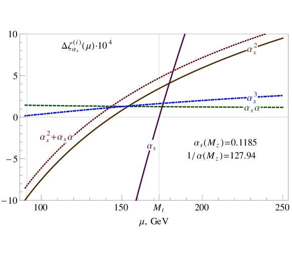
Figure 2: Scale dependence of different contributions to the ฮฑssubscript๐›ผ๐‘ \alpha_{s} matching relationย (20) around $\mu=M_{t}$. Boundary values for ฮฑsโ€‹(MZ)subscript๐›ผ๐‘ subscript๐‘€๐‘\alpha_{s}(M_{Z}) and $\alpha(M_{Z})$ are shown. The dependence of $\alpha$ on $\mu$ is neglected in (4โ€‹ฯ€)2โ€‹ฮ”โ€‹ฮถฮฑs(ฮฑsโ€‹ฮฑ)โ‰กฮฑsโ€ฒโ€‹ฮฑโ‹…ฮดโ€‹ฮถฮฑsโ€ฒโ€‹ฮฑ(2)superscript4๐œ‹2ฮ”superscriptsubscript๐œsubscript๐›ผ๐‘ subscript๐›ผ๐‘ ๐›ผโ‹…superscriptsubscript๐›ผ๐‘ โ€ฒ๐›ผ๐›ฟsuperscriptsubscript๐œsuperscriptsubscript๐›ผ๐‘ โ€ฒ๐›ผ2(4\pi)^{2}\Delta\zeta_{\alpha_{s}}^{(\alpha_{s}\alpha)}\equiv\alpha_{s}^{\prime}\alpha\cdot\delta\zeta_{\alpha_{s}^{\prime}\alpha}^{(2)}.

In order to demonstrate how the value of the calculated correction changes with the decoupling scale $\mu$ we plot the scale dependence of various contributions to relation (20) (see Fig.ย 2). For convenience, we introduce some obvious notation

ฮ”โ€‹ฮถฮฑs(ฮฑs)โ‰กฮฑsโ€ฒ(4โ€‹ฯ€)โ€‹ฮดโ€‹ฮถฮฑsโ€ฒ(1),ฮ”โ€‹ฮถฮฑs(ฮฑs2)โ‰กฮฑsโ€ฒโฃ2(4โ€‹ฯ€)2โ€‹ฮดโ€‹ฮถฮฑsโ€ฒ(2),etc.formulae-sequenceฮ”subscriptsuperscript๐œsubscript๐›ผ๐‘ subscript๐›ผ๐‘ superscriptsubscript๐›ผ๐‘ โ€ฒ4๐œ‹๐›ฟsuperscriptsubscript๐œsuperscriptsubscript๐›ผ๐‘ โ€ฒ1ฮ”subscriptsuperscript๐œsuperscriptsubscript๐›ผ๐‘ 2subscript๐›ผ๐‘ superscriptsubscript๐›ผ๐‘ โ€ฒ2superscript4๐œ‹2๐›ฟsuperscriptsubscript๐œsuperscriptsubscript๐›ผ๐‘ โ€ฒ2etc\Delta\zeta^{(\alpha_{s})}_{\alpha_{s}}\equiv\frac{\alpha_{s}^{\prime}}{(4\pi)}\delta\zeta_{\alpha_{s}^{\prime}}^{(1)},~{}\Delta\zeta^{(\alpha_{s}^{2})}_{\alpha_{s}}\equiv\frac{\alpha_{s}^{\prime 2}}{(4\pi)^{2}}\delta\zeta_{\alpha_{s}^{\prime}}^{(2)},~{}\mathrm{etc.} (22)

The RG evolution of ฮฑsโ€ฒโ€‹(ฮผ)superscriptsubscript๐›ผ๐‘ โ€ฒ๐œ‡\alpha_{s}^{\prime}(\mu) is found by means of four-loop RGEs for $n_{f}=5$ QCD and the scale dependence of the fine-structure constant is neglected. From Fig.ย 2 one can deduce that the electroweak correction is at the per myriad level and tends to decrease with the matching scale while pure QCD contributions become larger with $\mu$. At the scale $\mu=\mu_{0}\simeq 155$ย GeV they meet each other and for $\mu\gtrsim\mu_{0}$ the three-loop ๐’ชโ€‹(ฮฑs3)๐’ชsuperscriptsubscript๐›ผ๐‘ 3\mathcal{O}(\alpha_{s}^{3}) contribution becomes larger than the ๐’ชโ€‹(ฮฑsโ€‹ฮฑ)๐’ชsubscript๐›ผ๐‘ ๐›ผ\mathcal{O}(\alpha_{s}\alpha) terms. Moreover, it is interesting to note that at the same scale also the ๐’ชโ€‹(ฮฑs2)๐’ชsuperscriptsubscript๐›ผ๐‘ 2\mathcal{O}(\alpha_{s}^{2}) line crosses the meeting point. As a consequence, addition of the electroweak correction to the well-known ๐’ชโ€‹(ฮฑs2)๐’ชsuperscriptsubscript๐›ผ๐‘ 2\mathcal{O}(\alpha_{s}^{2}) expression doubles the two-loop QCD result.

One can also notice that the two-loop ๐’ชโ€‹(ฮฑsโ€‹ฮฑ)๐’ชsubscript๐›ผ๐‘ ๐›ผ\mathcal{O}(\alpha_{s}\alpha) contributions to the decoupling of ฮฑssubscript๐›ผ๐‘ \alpha_{s} at certain values of the matching scale can compete with the pure QCD corrections usually included in the RG analysis of the Standard Model. Due to this, for a precision study of the latter one has to take the calculated correction into account. However, one should keep in mind that to avoid double-counting it should be included only if the input value ฮฑsโ€ฒโ€‹(ฮผโˆผMZ)superscriptsubscript๐›ผ๐‘ โ€ฒsimilar-to๐œ‡subscript๐‘€๐‘\alpha_{s}^{\prime}(\mu\sim M_{Z}) is obtained from some low-energy observable.

It is also worth mentioning that recent re-analysis of the ALEPH data for hadronic $\tau$-decays [50] yields a value for ฮฑsโ€‹(mฯ„)=0.303โ€‹(14)subscript๐›ผ๐‘ subscript๐‘š๐œ0.30314\alpha_{s}(m_{\tau})=0.303(14), which is lower than the pre-averaged result ฮฑsโ€‹(mฯ„)=0.330โ€‹(14)subscript๐›ผ๐‘ subscript๐‘š๐œ0.33014\alpha_{s}(m_{\tau})=0.330(14) quoted in PDGย [32]. When evolved to the reference scale and matched with the SM by taking into account only QCD interactions of the $c-$, $b-$, and $t$-quarks it leads to a bit lower value for the SM strong coupling, which, in turn, could be accounted for (at least partially) by the inclusion of the electroweak contribution presented here.

To conclude, the two-loop ๐’ชโ€‹(ฮฑsโ€‹ฮฑ)๐’ชsubscript๐›ผ๐‘ ๐›ผ\mathcal{O}(\alpha_{s}\alpha) matching corrections for the strong coupling are calculated999The corresponding expressions in a computer-readable form can be found online as ancillary files of the arXiv version of the paper. and analyzed numerically. It is found that for the matching scale varying from 100 to 250 GeV the corrections tend to โ€œscreenโ€ the SM strong coupling, while the pure one- and two-loop QCD contributions lead to additional โ€œanti-screeningโ€ up to $\mu\lesssim 150-175$ GeV.

The corrections can play a role in reducing theoretical uncertainties of the running $\overline{\mathrm{MS}}$-coupling ฮฑssubscript๐›ผ๐‘ \alpha_{s} at the electroweak scale so that the SM can be tested in both the low-energy and high-energy region with increased accuracy.

Acknowledgments

We are grateful to A.V.ย Nesterenko, M.ย Kalmykov, O.ย Veretin, A.ย Pikelner, and B.Kniehl for fruitful discussions. We also thank S.ย Martin for pointing out a small typo in (18) and confirming our results in Ref.ย [51]. Furthermore, the author would like to thank 2nd Institute for Theoretical Physics of the University of Hamburg for hospitality while this article was being finished. This work is supported in part by RFBR grant 12-02-00412-a, the Ministry of Education and Science of the Russian Federation, Grant MK-1001.2014.2, Heisenberg-Landau Programme, and by the German Research Foundation through the Collaborative Research Center No.ย 676 Particles, Strings and the Early Universeโ€”The Structure of Matter and Space Time.

References

  • [1] S. Moch etย al., (2014), 1405.4781.
  • [2] G. โ€™tย Hooft, Nucl.Phys. B61 (1973) 455.
  • [3] T. van Ritbergen, J. Vermaseren and S. Larin, Phys.Lett. B400 (1997) 379, hep-ph/9701390.
  • [4] M. Czakon, Nucl.Phys. B710 (2005) 485, hep-ph/0411261.
  • [5] W. Bernreuther and W. Wetzel, Nucl.Phys. B197 (1982) 228.
  • [6] M. Steinhauser, Phys.Rept. 364 (2002) 247, hep-ph/0201075.
  • [7] A. Grozin, Int.J.Mod.Phys. A28 (2013) 1350015, 1212.5144.
  • [8] K. Chetyrkin, B.A. Kniehl and M. Steinhauser, Nucl.Phys. B510 (1998) 61, hep-ph/9708255.
  • [9] K. Chetyrkin, J.H. Kuhn and C. Sturm, Nucl.Phys. B744 (2006) 121, hep-ph/0512060.
  • [10] Y. Schroder and M. Steinhauser, JHEP 0601 (2006) 051, hep-ph/0512058.
  • [11] B. Kniehl etย al., Phys.Rev.Lett. 97 (2006) 042001, hep-ph/0607202.
  • [12] A.G. Grozin etย al., JHEP 1109 (2011) 066, 1107.5970.
  • [13] K. Chetyrkin, J.H. Kuhn and M. Steinhauser, Comput.Phys.Commun. 133 (2000) 43, hep-ph/0004189.
  • [14] F. Jegerlehner, M.Y. Kalmykov and B.A. Kniehl, Phys.Lett. B722 (2013) 123, 1212.4319.
  • [15] B.A. Kniehl and O.L. Veretin, Nucl.Phys. B885 (2014) 459, 1401.1844.
  • [16] G. Degrassi etย al., JHEP 1208 (2012) 098, 1205.6497.
  • [17] F. Bezrukov etย al., JHEP 1210 (2012) 140, 1205.2893.
  • [18] M.x. Luo and Y. Xiao, Phys.Rev.Lett. 90 (2003) 011601, hep-ph/0207271.
  • [19] L.N. Mihaila, J. Salomon and M. Steinhauser, Phys.Rev.Lett. 108 (2012) 151602, 1201.5868.
  • [20] K. Chetyrkin and M. Zoller, JHEP 1206 (2012) 033, 1205.2892.
  • [21] A. Bednyakov, A. Pikelner and V. Velizhanin, JHEP 1301 (2013) 017, 1210.6873.
  • [22] K. Chetyrkin and M. Zoller, JHEP 1304 (2013) 091, 1303.2890.
  • [23] A. Bednyakov, A. Pikelner and V. Velizhanin, Nucl.Phys. B875 (2013) 552, 1303.4364.
  • [24] A. Bednyakov, A. Pikelner and V. Velizhanin, Nucl.Phys. B879 (2014) 256, 1310.3806.
  • [25] A. Bednyakov, A. Pikelner and V. Velizhanin, Phys.Lett. B737 (2014) 129, 1406.7171.
  • [26] R. Harlander, L. Mihaila and M. Steinhauser, Phys.Rev. D72 (2005) 095009, hep-ph/0509048.
  • [27] A. Bednyakov, Int.J.Mod.Phys. A22 (2007) 5245, 0707.0650.
  • [28] A. Bauer, L. Mihaila and J. Salomon, JHEP 0902 (2009) 037, 0810.5101.
  • [29] A. Kurz, M. Steinhauser and N. Zerf, JHEP 1207 (2012) 138, 1206.6675.
  • [30] A. Bednyakov, Int.J.Mod.Phys. A25 (2010) 2437, 0912.4652.
  • [31] D. Noth and M. Spira, JHEP 1106 (2011) 084, 1001.1935.
  • [32] Particle Data Group, K. Olive etย al., Chin.Phys. C38 (2014) 090001.
  • [33] A. Pich, (1998) 949, hep-ph/9806303.
  • [34] S. Larin, T. van Ritbergen and J. Vermaseren, Nucl.Phys. B438 (1995) 278, hep-ph/9411260.
  • [35] S. Fleming etย al., Phys.Rev. D77 (2008) 074010, hep-ph/0703207.
  • [36] J. Fleischer and F. Jegerlehner, Phys.Rev. D23 (1981) 2001.
  • [37] M. Awramik etย al., Phys.Rev. D68 (2003) 053004, hep-ph/0209084.
  • [38] R. Hempfling and B.A. Kniehl, Phys.Rev. D51 (1995) 1386, hep-ph/9408313.
  • [39] F. Jegerlehner, M.Y. Kalmykov and O. Veretin, Nucl.Phys. B658 (2003) 49, hep-ph/0212319.
  • [40] L.R. Surguladze, (1996), hep-ph/9803211.
  • [41] D.J. Gross and F. Wilczek, Phys.Rev.Lett. 30 (1973) 1343.
  • [42] H.D. Politzer, Phys.Rev.Lett. 30 (1973) 1346.
  • [43] W.E. Caswell, Phys.Rev.Lett. 33 (1974) 244.
  • [44] D. Jones, Nucl.Phys. B75 (1974) 531.
  • [45] O. Tarasov and A. Vladimirov, Sov.J.Nucl.Phys. 25 (1977) 585.
  • [46] E. Egorian and O. Tarasov, Teor.Mat.Fiz. 41 (1979) 26.
  • [47] T. Hahn, Comput.Phys.Commun. 140 (2001) 418, hep-ph/0012260.
  • [48] A.I. Davydychev and J. Tausk, Nucl.Phys. B397 (1993) 123.
  • [49] K. Chetyrkin and F. Tkachov, Nucl.Phys. B192 (1981) 159.
  • [50] D. Boito etย al., (2014), 1410.3528.
  • [51] S.P. Martin, (2018), 1812.04100.