On the Consistency of Approximate Quantum Dynamics Simulation Methods for Vibrational Spectra in the Condensed Phase

Abstract

Including quantum mechanical effects on the dynamics of nuclei in the condensed phase is challenging, because the complexity of exact methods grows exponentially with the number of quantum degrees of freedom. Efforts to circumvent these limitations can be traced down to two approaches: methods that treat a small subset of the degrees of freedom with rigorous quantum mechanics, considering the rest of the system as a static or classical environment, and methods that treat the whole system quantum mechanically, but using approximate dynamics. Here we perform a systematic comparison between these two philosophies for the description of quantum effects in vibrational spectroscopy, taking the Embedded Local Monomer (LMon) model and a mixed quantum-classical (MQC) model as representatives of the first family of methods, and centroid molecular dynamics (CMD) and thermostatted ring polymer molecular dynamics (TRPMD) as examples of the latter. We use as benchmarks D₂O doped with HOD and pure H₂O at three distinct thermodynamic state points (ice Ih at 150K, and the liquid at 300K and 600K), modeled with the simple q-TIP4P/F potential energy and dipole moment surfaces. With few exceptions the different techniques yield IR absorption frequencies that are consistent with one another within a few tens of cm^-1. Comparison with classical molecular dynamics demonstrates the importance of nuclear quantum effects up to the highest temperature, and a detailed discussion of the discrepancies between the various methods let us draw some (circumstantial) conclusions about the impact of the very different approximations that underlie them. Such cross validation between radically different approaches could indicate a way forward to further improve the state of the art in simulations of condensed-phase quantum dynamics.

The simulation of nuclear quantum dynamics in the condensed phase remains a challenge even for state of the art methods. The main problem is that the dimensionality of these systems is too large for a fully “first-principles” quantum calculation of the nuclear dynamics, leaving the whole field without a reliable benchmark. Therefore, it is hard to assess how well different approximations perform even for exhaustively studied systems like bulk water. There is a dire need to find a reliable framework in which the quantum dynamics of these systems can be treated, so that the field can advance further.

One can identify at least two classes of popular methods to model quantum dynamics in the condensed phase. The first treats a subset of the system’s degrees of freedom fully quantum mechanically, embedded in the electrostatic environment of the rest of the system. Examples of these methods are the local monomer approximation (LMon) Wang and Bowman (2011, 2012), which treats quantum mechanically a small subset of all intramolecular degrees of freedom in a static environment, and a mixed quantum-classical (MQC) model based on the semi-classical theory of line shape, that treats a single degree of freedom (e.g. an OH stretch) “on-the-fly” in the presence of perturbing electric field generated by the surrounding classical solvent Torii (2006); Skinner, Auer, and Lin (2009); Gruenbaum et al. (2013). The second class of methods treats the whole system on the same footings, but using (physically motivated) ad hoc approximations to the quantum dynamics. These methods are often based on classical trajectories initiated from quantum distributions Miller (2005); Liu and Miller (2006); Liu et al. (2009), or are inspired by imaginary time path integral molecular dynamics (PIMD), as in the cases of centroid molecular dynamics (CMD)Cao and Voth (1994); Jang and Voth (1999) and (thermostatted) ring polymer molecular dynamics (TRPMD)Craig and Manolopoulos (2004); Habershon et al. (2013); Rossi, Ceriotti, and Manolopoulos (2014). Since these two classes of approaches are grounded on very different approximations, a comparison between their results is perhaps the closest one can get to assess their reliability in the absence of an absolute, exact benchmark Paesani and Voth (2010); Ahlborn et al. (1999).

Here we perform such cross-validation, comparing the behavior of MQC, LMon, CMD, and TRPMD when modeling a physical observable that is particularly sensitive to the description of nuclear quantum dynamics – the infra-red absorption spectra of hydrogen-containing compounds Habershon, Fanourgakis, and Manolopoulos (2008); Witt et al. (2009); Ivanov et al. (2010); Paesani and Voth (2010); Rossi, Ceriotti, and Manolopoulos (2014). We focused on prototypical hydrogen-bonded condensed phase systems – HOD in D₂O and neat water – describing them with the inexpensive q-TIP4P/F potential Habershon, Markland, and Manolopoulos (2009), and using the corresponding linear dipole moment surface (DMS) to evaluate the IR absorption. The rationale for this simplistic choice is that we are not so much interested in comparing with experimental data, but only to nail down differences between methods for condensed-phase quantum dynamics. The simplicity of the potential and the linear DMS make it possible to guarantee thorough statistical sampling and to focus on the problem of modeling the dynamics on a complex, anharmonic potential energy surface, rather than on the fact that CMD and (T)RPMD are much harder to justify when computing correlation functions of non-linear operators Jang, Sinitskiy, and Voth (2014); Braams and Manolopoulos (2006); Hele and Althorpe (2013). It also allows us to test extensively the dependence of TRPMD, CMD, and LMon to the precise details of the calculations. To validate the two philosophies over a broad range of conditions, and draw conclusions that are not purely anecdotal, we considered three very different thermodynamic regimes: ice Ih at 150K, liquid water at 300K, and the hot liquid at 600K at the experimental liquid/vapor coexistence density. To assess the importance of these approximate nuclear quantum dynamics, we also compare our results to classical MD simulations.

CMD and TRPMD simulations were performed using the i-PI code Ceriotti, More, and Manolopoulos (2014), and LAMMPS as the force back-end Plimpton (1995). The details of the q-TIP4P/F potential are available elsewhere Habershon, Markland, and Manolopoulos (2009), as well as the technical details of the integration and thermostatting of PIMD Ceriotti et al. (2010). We also performed classical MD reference calculations, using a time step of 0.5 fs and a weak global thermostat Bussi, Donadio, and Parrinello (2007). For both TRPMD and CMD we applied a Langevin thermostat to the internal modes of the ring polymer. In TRPMD we set the friction coefficients equal to the free ring-polymer frequencies: $\gamma_{k}=\omega_{k}$. We made this choice as a compromise between the damping of spurious peaks in the spectrum and the broadening of the physical peaks Rossi, Ceriotti, and Manolopoulos (2014), and used a time step of 0.25 fs. In our CMD calculations we scaled the dynamical masses of the internal modes of the ring polymer to shift all the frequencies to the common value $\Omega=16000$cm^-1, and used a time step of 0.025fs, which makes CMD simulations ten times more demanding than TRPMD for the same level of statistics. CMD has better sampling efficiency than plain RPMD due to the thermostatting of the ring polymer normal modes Pérez, Tuckerman, and Müser (2009), but the efficiency of TRPMD should be comparable since it uses an analogous thermostat. In running the CMD calculations we noticed that the details of the thermostat have a significant impact on the centroid dynamics. As discussed in the Supplementary Material (SM)sm , the commonly-adopted prescription of optimal coupling of either Langevin or Nosé-Hoover thermostats with the shifted frequency interferes with adiabatic decoupling at least up to $\Omega\leq 16000$ cm^-1 in the cases studied here. We found that in the limit of weak thermostat coupling ($\lambda=0.01$), proper adiabatic separation can be reached already at $\Omega<8000$ cm^-1, which could probably enable using longer time steps. This should be considered when performing CMD calculations and when comparing with existing results.

All our LMon calculations were performed using the MULTIMODE codeCarter, Culik, and Bowman (1997); Carter, Bowman, and Handy (1998); Bowman, Carter, and Huang (2003). The LMon method assumes it is possible to take a snapshot configuration of a condensed-phase system, and solve exactly the Schrödinger equation for a subset of its degrees of freedom, evaluating the changes of the potential as a function of deformations of a molecule along a subset of its “lormal” modes. A detailed explanation of this approach can be found for instance in Ref.Wang and Bowman (2011). The LMon approximation makes it possible to progressively include more physics by increasing the dimensionality of the quantum subspace. Using just the three intra-molecular “lormal” modes as the quantum-mechanical subspace (LMon-3) is generally sufficient to describe the stretching and bending regions of the spectrum of waterLiu, Wang, and Bowman (2014a). A recent study of vibrational energy relaxation (VER) of dilute HOD in ice Ih considered also three additional intermolecular modes (LMon-6)Liu, Wang, and Bowman (2014b), obtaining a description of the intermolecular vibrational spectrum and an improved accuracy in the intra-molecular region, but at a much higher computational cost. Here we are mostly interested in the strongly-quantized intra-molecular vibrations, and so we attempted a simplified approach that uses a total of four modes (LMon-4). Hundreds of monomer+environment configurations were obtained from individual replicas of a series of PIMD simulations. For each snapshot, the three intramolecular modes are complemented with the three highest-frequency inter-molecular modes, that are however considered one at a time: for each monomer, 3 sets of LMon-4 calculations are performed separately. A smooth spectrum is obtained by combining Gaussian line shapes centered around the energies of transitions from the ground state to each of the excited states, weighed by the transition dipole moment. Further numerical details about all the calculations can be found in the SM.

MQC calculations were performed with an in-house code. Following Ref Paesani and Voth (2010), several independent CMD trajectories were performed starting from equilibrated PIMD configurations, from which the time-dependence of the vibrational frequency and transition dipole moment for the OH stretch were computed. The semiclassical vibrational line shape was then evaluated as discussed in Ref. Mukamel (1999), including non-Condon corrections as defined, e.g., in Ref. Schmidt, Corcelli, and Skinner (2005). A more detailed description of the simulations, as well as a discussion of the importance of non-Condon corrections, is reported in the SM. From the point of view of computational cost, both MQC and LMon-4 are relatively inexpensive, the most demanding aspect being the preliminary (PI)MD simulation. Traditionally the environment is sampled classically – which particularly at low temperature can be orders of magnitude less demanding – but as we will see results are influenced by the classical or quantum treatment of the environment. Then, the evaluation of the stretching frequency in MQC is trivial, for such a simple potential. Each LMon-3 calculation takes a few seconds on a single core, and about one minute for LMon-4. The cost would increase steeply as a function of the size of the quantum subspace, but up to LMon-6 the cost will most likely be dominated by the preliminary sampling of bulk configurations.

Let us start by considering a single HOD molecule solvated in D₂O. This system (and its counterpart, HOD in H₂O) is commonly used as a probe for studying the local structure of liquid water theoretically and experimentally Bakker and Skinner (2009); Paesani and Voth (2010). The OH stretch is dynamically uncoupled with the environment, making this system well-suited for both MQC and LMon calculations Liu, Wang, and Bowman (2014b).

The results for classical MD, CMD, TRPMD, MQC and LMon are shown in Figure 1. Starting from the highest temperature, 600 K, with a hot and compressed liquid, we observe that classical MD is blue-shifted by around 50 cm^-1 with respect to all quantum methods. Even at this high temperature nuclear quantum effects affect the calculation of dynamical properties. The blue shift of the classical simulation gets more pronounced by lowering the temperature, as expected, amounting to approximately 100 cm^-1 at 150K. At 600 K all quantum methods show a large blue-shift, increased band width and asymmetric or structured line shapes, compared to those at 150 and 300 K. The LMon-4 band intensity falls-off faster than other line shapes at the high-frequency edge of the band, and shows a sharper maximum which is 30-50 cm^-1 to the ”blue” of the CMD and TRPMD maxima, which are not sharp. Considering that the influence of low-frequency intermolecular modes, e.g., hot bands, additional dipole variation, vibrational relaxation, etc., becomes more important with increasing temperature and that LMon-4 is only partially describing this coupling, the limitations in the LMon- 4 theory are also expected to be become more apparent. The importance of inter-molecular couplings and of the dynamics of the environment at the higher temperature is also suggested by the large difference we observe between the MQC line shape, the Condon approximation to the MQC line shape, and MQC vibrational density of states (VDOS, see the SM).

At 300 K the agreement between different quantum techniques is perhaps even better. MQC and CMD overlap almost perfectly. The LMon peak is some 20-40 cm^-1 higher in frequency, and the difference between the LMon and MQC line shapes is much less dramatic than at 600K. At 300 K, inhomogeneous broadening effects (i.e., effects not related to vibrational relaxation or motional narrowing) are dominant. The TRPMD peak is further blue-shifted (by 20-40 cm^-1, depending on whether one considers the maximum or the mean position of the peak) and artificially broadened by the strong thermostatting of non-centroid modes.

In ice Ih at 150K TRPMD and LMon still are in remarkable - although perhaps fortuitous - agreement. CMD shows a pronounced red shift of 180 cm^-1, which should probably be attributed to the curvature problem Witt et al. (2009); Rossi, Ceriotti, and Manolopoulos (2014). The MQC peak is red-shifted by about 60 cm^-1 relative to LMon and TRPMD. One possible explanation for this shift is the description of the environment based on centroid configurations, that are very close to classical. Contrary to higher temperatures, the LMon spectrum also depends on whether the environment configurations are obtained from the beads of the PIMD simulation, or from the centroid. In the latter case, as when using configurations from classical MD, the OH stretch peak is red-shifted by 25 cm^-1 (see the SM). It is arguable which choice is more physically justified. On one hand, bead positions provide a statistically accurate snapshot of the quantum environment. On the other, centroids can be seen as a mean-field average of the quantum fluctuations of the neighboring molecules, closer perhaps to the spirit of a quantum-classical model. In the absence of a rigorous justification we can see this discrepancy as a sign of the break-down of the classical model for the environment, and consider the difference between the two spectra as an estimate of the reliability of LMon (and MQC) in this low temperature regime.

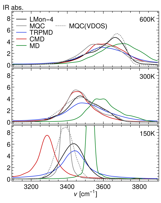
Figure 1: Comparison between the OH stretch IR absorption spectrum for a single HOD molecule in bulk D₂O, modeled using the q-TIP4P/F potential. Absorption spectra were computed from the dipole derivative autocorrelation, using classical molecular dynamics (green), CMD (red), and TRPMD (blue), and compared with the results of LMon-4 calculations (black) and MQC line shape (gray) and VDOS (gray dotted). The panels correspond, from top to bottom, to liquid water at 600 K, liquid water at 300 K and ice Ih at 150 K. The integrated intensity of the OH stretch peak has been normalized to the same area.

Having compared all methods for the HOD:D₂O benchmark, we consider in Fig. 2 the spectra of water in the three thermodynamic regimes discussed above. We did not perform MQC simulations, since the isolated chromophore assumption is less justified in H₂O. Let us start by discussing the OH band, that shows similar trends to those observed for HOD in heavy water. At 600K, CMD and TRPMD are in near-perfect agreement, and the peak maxima are slightly red-shifted relative to LMon-4 by about 50 cm^-1. This is consistent with our observations in HOD case, and the discrepancy can be attributed to the lack of homogeneous broadening and dynamical couplings in LMon. At 300K TRPMD and LMon-4 are close to each other, while CMD shows a small red shift of less than 50 cm^-1, consistently with what observed in HOD:D₂O. In the case of low-temperature ice the CMD peak is red shifted by 150 cm^-1 compared to both LMon-4 and TRPMD, that agree well with each other – even though the TRPMD peak is considerably broader. The intensity of the stretching band is much under-estimated relative to experiments. This is due to the linear DMS of q-TIP4P/F, as evidenced by comparison with more sophisticated models Wang et al. (2011), but is irrelevant for our comparison of approximate methods for quantum dynamics.

Moving on to the bend, we observe good agreement in the peak position and width among all the quantum methods. All predict a slight red shift with increasing temperature (in qualitative agreement with experiment). TRPMD and CMD give peaks positions at 1640 cm^-1 at 150 K and about 1610 cm^-1 in at 600 K. LMon-4 gives 1640 cm^-1 at 150 K and 1590 at 600 K. The peak at 600K is further lowered to 1570cm^-1 when using LMon-3 (see the SM), indicating the growing importance of inter-molecular coupling at high temperature, and suggesting that this slight discrepancy between LMon-4 and PIMD-based methods could be resolved by increasing further the dimensionality of the quantum subspace. Finally, in the low-frequency region CMD and TRPMD are almost identical. In this region one cannot expect LMon-4 to yield quantitative accuracy. The quantum sub-space does not contain the collective modes of the hydrogen-bond network, nor the translation modes of individual monomers.

Within the LMon scheme it is straightforward to treat effects beyond linear absorption, and to give a clear physical attribution of specific features of the spectrum. For instance, all of the spectra display a distinct bump or shoulder around 3200 cm^-1, which corresponds to the first overtone of the bend. An interesting feature captured by LMon-4 (but not by LMon-3) is the small peak around 2350 cm^-1, which is evident at 150K and becomes less clear-cut with raising temperature. This feature, is due to the combination band of bending and librational modes, and demonstrates how increasing the dimensionality of the quantum subspace rogressively includes additional physical effects in LMon calculations. Both CMD and TRPMD display non-zero absorption in this region, but further analyses would be needed to attribute that spectral density to a precise physical origin.

Figure 2: Infra-red absorption spectrum of H₂O at three different thermodynamic conditions. From top to bottom: (compressed) liquid water at 600 K, liquid water at 300 K and ice Ih at 150 K. The curves correspond to TRPMD (blue), CMD (red) and LMon-4 calculations (black). Note in the middle panel the reduced red shift of the OH peak in CMD compared with the results in Ref. Rossi, Ceriotti, and Manolopoulos (2014). The coupling of efficient thermostats with the internal modes of the ring polymer, that was used in the previous work, caused a spurious red shift of about 30 cm^-1 (see also the SM).

The conclusions of our comparison of approximate quantum dynamics simulation methods are overall optimistic: all the methods we considered are generally consistent with each other, while the difference with the position of the OH stretching peak observed in classical molecular dynamics confirms the importance of including nuclear quantum effects to reproduce quantitatively spectroscopic measurements of hydrogen-containing systems. TRPMD and LMon agree within a few tens of cm^-1 over a range of thermodynamic conditions going from ice Ih at 150K to water at 300K and finally to the hot, compressed liquid at 600K. So do CMD down to room temperature, and MQC in the cases where it is applicable. Furthermore, this analysis reinforces the notion that performing PIMD-based and quantum-subspace simulations in tandem does not only provide a degree of cross-validation, but also makes it possible to profit simultaneously from the complete (albeit approximate) description of the absorption spectrum given by the former family of methods, and from the interpretation of distinct spectral features that is enabled by an explicit quantum treatmentPaesani, Xantheas, and Voth (2009).

The comparison between the different methods also highlights their current limitations, and suggests that results of quantum dynamics should always be interpreted with caution. Extensions of MQC beyond the case of an isolated chromophore require one to model the interaction between the different chromophores, either explicitly or by devising an effective mapping of the molecular Hamiltonian on a collective coordinate, such as the local electrostatic potentialChoi and Cho (2013). Even though LMon can in principle be improved systematically, its computational cost increases exponentially with the size of the quantum subspace, making it challenging to fully assess the importance of inter-molecular couplings. Treating the environment semiclassically, in the same spirit as the MQC model, might be a better way to account for inter-molecular dynamical effects. One has also to consider that the present work represents the first application of LMon to a finite-temperature scenario. More work is needed to include systematically a description of monomer-monomer couplings, hot bands and the dynamical nature of the environment. Particularly at the highest temperature, these effects may affect the line shape of the absorption peaks, as highlighted by the comparison with MQC. We also observe that at 150K the results of a LMon calculation depends sizably on whether one takes snapshots of the environment that are consistent with quantum statistics (e.g., from the beads in an PIMD simulation) or that are essentially classical (e.g., taken from classical MD, or using the ring polymer centroids).

Methods inspired by PIMD also have their issues. In its straightforward partially-adiabatic implementation, CMD requires a small integration time step, and one should pay attention to the fine details of the thermostatting to avoid interfering with the adiabatic decoupling of the centroid. At low temperatures, a pronounced red-shift relative to all other methods is observed. The precise temperature where this artifact becomes sizable should depend on the details of the system being studied. TRPMD, on the other hand, can be straightforwardly used with the same time step of a PIMD calculation, and does not suffer from systematic low-temperature red shifts. However, the OH stretch mode can be up to 50cm^-1 blue-shifted relative to some of the other techniques. Furthermore, the precise peak position varies depending on the choice of the thermostat coupling, which is somewhat arbitrary. The strong thermostatting that is used to fix the resonance problems of RPMD also leads to a significant broadening of the peaks, so the TRPMD line shape should not be taken too seriously, unless it is dominated by inhomogeneous broadening or is weakly quantized.

Our results give some confidence on the reliability of approximate quantum dynamical methods for simulating the dynamics and the spectroscopy of condensed-phase systems or large molecules. The difference between quantum and classical simulations is comparable to the errors due to imperfect potentials, but the discrepancies between different quantum methods are less important. The best agreement between the various methods is seen for liquid water at room temperature – perhaps unsurprisingly considering that it corresponds to the regime for which most of approximate quantum techniques were designed. Cross-validation between different approaches, particularly at thermodynamic conditions outside of their “comfort zone”, offers the best promise for demonstrating the accuracy of existing methods, for uncovering their errors and shortcomings, and for delivering more reliable, simple and affordable simulation strategies.

I Acknowledgements

We gratefully acknowledge stimulating discussion with David Manolopoulos, Gregory Voth, and Lu Wang. MR thanks the Deutsche Forschungsgemeinschaft (DFG), RO 4637/1, for funding. HL and JMB thank the US National Science Foundation, CHE-1145227, for funding. FP thanks the US National Science Foundation, CHE-1111364, for funding, and the Extreme Science and Engineering Discovery Environment (OCI-1053575, TG-CHE110009) for computational time.

Appendix A Details of TRPMD and CMD simulations

It is well known from Fermi’s golden rule that the IR spectrum can be obtained by McQuarrie (2000)

$$n(\omega)\alpha(\omega)=\frac{\pi\omega}{3\hbar cV\epsilon_{0}}(1-e^{-\beta\hbar\omega})I_{\mu\mu}(\omega)$$ (1)

$$I_{\mu\mu}(\omega)=\frac{1}{\pi}\int_{0}^{\infty}e^{i\omega t}\langle\bm{\mu}(0)\cdot\bm{\mu}(t)\rangle dt$$ (2)

where $\mu$ is the dipole moment, $n(\omega)$ the refractive index, $\alpha(\omega)$ the Beer-Lambert absorption coefficient, and $V$ the volume of the simulation box. The angular brackets indicates a canonical average. TRPMD and CMD can be better described as approximations to the Kubo-transform time correlation, which is given by Habershon, Fanourgakis, and Manolopoulos (2008)

$$\tilde{c}_{\mu\mu}(t)=\frac{1}{\beta}\int_{0}^{\beta}d\lambda\langle\bm{\mu}(-i\lambda\hbar)\cdot\bm{\mu}(t)\rangle$$ (3)

that has a simple Fourier transform relation to the canonical autocorrelation function given by

$$\tilde{I}_{\mu\mu}(\omega)=\frac{(1-e^{-\beta\hbar\omega})}{\beta\hbar\omega}I_{\mu\mu}(\omega)$$ (4)

where $\tilde{I}_{\mu\mu}(\omega)$ is the Fourier transform of Eq. 3. The final expression is, thus

$$n(\omega)\alpha(\omega)\propto\omega^{2}\tilde{I}_{\mu\mu}(\omega).$$ (5)

Instead of using directly the equation above to calculate our spectra with the Fourier transform of the dipole autocorrelation, we have instead calculated the Fourier transform of the autocorrelation of the dipole time derivative. These two quantities are related by

$$\tilde{I}_{\dot{\mu}\dot{\mu}}(\omega)=\omega^{2}\tilde{I}_{\mu\mu}.$$ (6)

The time derivative was taken numerically from two consecutive time steps and the final expression we used for the IR spectra shown in the paper is thus

$$n(\omega)\alpha(\omega)\propto\tilde{I}_{\dot{\mu}\dot{\mu}}(\omega).$$ (7)

Since the dipole is only a function of positions $\mathbf{q}$, in the path-integral based approximations, the estimator for the dipoles is given by $\bm{\mu}=1/P\sum_{i=1}^{P}\bm{\mu}_{P}(\mathbf{q})$, where $i$ runs through the $P$ replicas (beads) of the ring polymers. In the q-TIP4P/f model used here the dipole is linear with respect to the positions, such that we could take simply the dipole moment of the centroid configurations in the expression above.

Given the difficulty of directly comparing the spectra coming from all different approaches treated in the manuscript, we have normalized the integrated intensity of all spectra to be the same.

We performed initial equilibration runs of 100 ps in order to obtain starting structures for the TRPMD and CMD simulations for all system at each temperature studied. For HOD:D₂O ice at 150K we performed 8 independent initial runs with H in different positions in order to account for proton disorder. We disregarded the first 5 ps of each thermalization run and took starting geometries (5 to 10 ps apart) from the rest of these simulations. Starting geometries for CMD and TRPMD were taken from the same thermalization runs in each case, and several independent runs were performed. In total, for HOD:D₂O we ran 20 ns of simulations for TRPMD and 6 ns for CMD for each temperature – a very long time to ensure the convergence of the spectra, which is especially difficult in this case since we could not exploit horizontal statistics. We calculated the HOD IR absorption spectrum from the dipole of the HOD molecule only. For H₂O we performed 100ps of TRPMD and 100ps of CMD for each temperature, since here we could exploit horizontal statistics. We obtained the IR spectrum from the total dipole moment of the cell.

The time step used for these simulations was 0.5 fs for MS, 0.25fs for TRPMD and 0.025fs for CMD. In all cases, to improve ergodicity, we attached to the atoms or the centroid a weak global thermostat that has been proven not to affect dynamical properties Bussi, Donadio, and Parrinello (2007). The number of beads used for ice Ih at 150 K was 64, and we took a box containing 96 water molecules at the experimental structure and density. For the liquid at 300 K we used 32 beads and a box containing 128 water molecules, also at experimental density. For the high temperature simulation at 600K we used 16 beads, a box of 128 water molecules, and the experimental density at the liquid-vapor coexistence at this temperature.

For the Fourier transform of the dipole autocorrelation series we used a lag of 1 ps and padded the signal with zeros in order to obtain a grid of around 3 cm^-1 in frequency space. We also windowed the autocorrelation function with a Hanning window in order to filter spurious ringings of the signal.

Appendix B Details of LMon calculations

As discussed in the text, we opted here for a compromise on the size of the quantum subspace, using the LMon-4 as an effective approximation to LMon-6. For each monomer, 3 sets of LMon-4 calculations are performed separately. Each LMon-4 calculation yields a series of energy states, and the corresponding matrix of transition dipole moments. Since we consider each snapshot three times, using a different inter-molecular mode but the same intramolecular modes, the approach lead to an over-estimation of the intensity of intramolecular absorptions. To avoid this overcounting we weighted all the transitions from the ground state to intramolecular excited states by a factor of 1/3. Transitions to states with non-zero quanta in the intermolecular mode correspond to different quantum mechanical states in each of the three LMon-4 calculations, so their intensity has been weighed in full.

For dilute HOD in D₂O water, only the HOD monomer was consider for the LMon-4 calculations. In the case of ice we took configurations from eight independent realizations of the lattice to sample different electrostatic environments for the HOD molecule. For pure H₂O water, 5 monomers are sampled from each snapshot. The snapshots are between 0.5 and 1 ps apart from each other in order to ensure a better statistical sampling. The total numbers of monomer configurations for HOD are 2185, 1132 and 1165 for 150K, 300 K and 600 K respectively. For H₂O, the numbers are 2400, 1951 and 1486 for 150K, 300 K and 600 K respectively. The final spectra were smoothed with a Gaussian function with FWHM=50 cm^-1. This amplitude is much smaller than the intrinsic bandwidth of the features of the spectrum of water, and we only used it to eliminate the noise due to the use of a finite number of monomer configurations.

As discussed in the main text – for the relatively small dimensionality of quantum subspace we used – the main bottleneck is the preliminary sampling of bulk configurations. This is particularly true when performing such sampling using path interal molecular dynamics, that depending on the implementation and the temperature might be orders of magnitude more demanding than classical molecular dynamics.

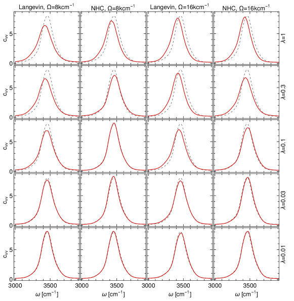
Figure S1: OH-stretching peak for the centroid velocity correlation spectrum in a PA-CMD simulation of liquid water at room temperature. The different panels correspond to different NM dynamical frequency $\Omega$ and thermostat strength $\lambda$. The dashed line correspond to an average of the peaks obtained with $\lambda=0.01$, and is plotted as to guide to the eye.

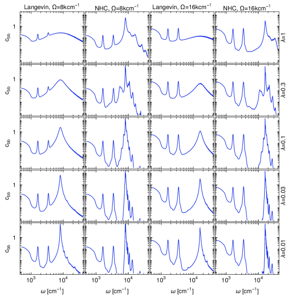
Figure S2: Velocity-velocity correlation function for one of the beads in a PA-CMD simulation of liquid water at room temperature. The different panels correspond to different NM dynamical frequency $\Omega$ and thermostat strength $\lambda$. The plots are reported on a log-log scale, to visualize clearly the different time scales involved.

Appendix C Assessing the effect of normal-modes thermostatting in CMD

Centroid molecular dynamics is defined as the (microcanonical) dynamics of the ring polymer centroid on the potential of mean force obtained by averaging the ring polymer Hamiltonian over the possible fluctuations of the beads with fixed centroid position Cao and Voth (1994).

In practical implementations, one does not average explicitly over the internal modes of the ring polymer, but performs a simultaneous dynamics of the centroid and the non-zero frequency normal modes (NM) of the free ring polymer, defining the dynamical masses in such a way that (for a free particle) all the normal modes vibrate at a common frequency $\Omega$. By setting this frequency to a value much larger than any physical vibration in the system, one obtains a (partial) adiabatic decoupling between the centroid and the other NM (PA-CMD), i.e. the ring polymer potential energy surface is sampled dynamically as the centroid moves on a much slower time scale Hone and Voth (2004).

As a consequence of this rescaling of the dynamical masses, one has to use smaller time steps to integrate the equations of motion – that get smaller the larger the maximum dynamical frequency is. It is worth noting that the time scale for the integration is not determined by the value of $\Omega$ alone, but by a combination of $\Omega$, inverse temperature $\beta$, and the maximum physical frequency present in the system, $\omega_{\text{max}}$. In fact, before the mass scaling, the slowest internal mode of the free ring polymer has a frequency of approximately $2\pi/\beta\hbar$. In the presence of an external harmonic potential with frequency $\omega_{\text{max}}\gg 2\pi/\beta\hbar$, its intrinsic vibrational frequency shifts to approximately $\omega_{\text{max}}$. Since the mass-scaling acts on all the physical degrees of freedom, and scales all the ring polymer vibrations by the same factor, irrespective of the underlying physical potential, a PA-CMD simulation of the system described above will contain a vibrational mode whose dynamical frequency is approximately $\Omega\omega_{\text{max}}\beta\hbar/2\pi$. For moderately quantum systems this is much larger than $\Omega$ itself.

The choice of the NM frequency $\Omega$ is generally understood to be crucial to obtain convergence of the dynamical properties computed by PA-CMD to the fully adiabatic values, while maintaining a compromise between the converged result and the use of a reasonably large time step. Any work based on PA-CMD quotes clearly the value of $\Omega$, or an equivalent adiabaticity parameter that conveys the same information Hone and Voth (2004). However, if PA-CMD is meant to perform an on-the-fly average of the ring-polymer potential, the NM have to be properly thermostatted. The common wisdom is then to use a thermostat that is optimally coupled to the dynamical frequency $\Omega$, in order to sample the potential of mean force as efficiently as possible. For instance, when using a Nosé-Hoover chains thermostat Hoover (1985); Nosé (1984); Martyna, Klein, and Tuckerman (1992), one should set the thermostat mass to $Q=P/\beta\Omega^{2}$ Kinugawa, Moore, and Klein (1997). When using a Langevin thermostat one should set the friction to the critical damping $\gamma=2\Omega$Ceriotti et al. (2010).

Having observed difficulties in converging PA-CMD results with respect to $\Omega$ while using an optimally-coupled Langevin thermostat, we have performed an extensive investigation of how the centroid velocity correlation spectrum computed by PA-CMD depends separately on $\Omega$ and on NM thermostatting, for a simple flexible water model Habershon, Markland, and Manolopoulos (2009), at a temperature of 300K, using 32 beads and a time step of 0.025fs. We describe the intensity of the coupling by a parameter $\lambda$, that is defined as $\lambda=\gamma/2\Omega$ for Langevin thermostatting, and as $\lambda^{2}=P/\beta Q\Omega^{2}$ for Nosé-Hoover thermostatting (chains of four thermostats, one chain per degree of freedom). In both cases, the parameter corresponds to optimal coupling to a scaled frequency $\lambda\Omega$, so that smaller $\lambda$ corresponds to weaker coupling.

Figure S1 shows the results of this analysis. The amplitude and position of the OH stretching peak depends significantly on the NM thermostatting, both for Langevin and Nosé-Hoover thermostats. As $\lambda$ decreases, the peaks shift progressively to higher frequency, until converged results are reached in a weak coupling regime with $\lambda\approx 0.01$. This turns out to be the proper adiabatically-decoupled limit, and the peak position and shape does not change significantly if $\lambda$ is further decreased, or $\Omega$ further increased. This effect is very insidious, since in the limit of a strong thermostat the position changes very little when $\Omega$ is increased, which may give the impression that adiabatic decoupling has been reached. In fact, recent results by some of the Authors were obtained with $\Omega=16000$cm^-1 and $\lambda=0.2$, and were therefore red-shifted by about 30cm^-1 relative to the correct fully adiabatic limit – thereby exaggerating the curvature problem Rossi, Ceriotti, and Manolopoulos (2014).

The origin of this strong thermostat dependence can be understood by looking at the overall dynamical behavior of the thermostatted ring polymer. Figure S2 shows the bead velocity correlation spectrum, that displays signatures of the motion of all the ring polymer degrees of freedom simultaneously. One can notice clearly a large peak corresponding to the target NM frequency $\Omega$ and also, for weak couplings, the presence of additional peaks at much higher frequency that correspond to the combination of the physical potential with the spring terms in the path integral Hamiltonian.

However, the NM vibrations are altered by the presence of a strong thermostat, that broadens the vibrational peak and causes spurious interactions between the internal modes and the centroid. This is reminiscent of the effect of a thermostat in Car-Parrinello molecular dynamics, where the use of a white-noise Langevin thermostat disrupts the adiabatic decoupling between the ionic and electronic degrees of freedom Ceriotti, Bussi, and Parrinello (2009). This effect is very evident in the case of Langevin thermostatting, while the impact of NHC thermostats on the dynamics is more subtle. The fact that NHC thermostats alter the peak shape nearly as much as Langevin dynamics can be probably be understood by the fact that NH equations are non-linear, and therefore not invariant to unitary transformations of the coordinates Ceriotti et al. (2010), and so they lead to stronger coupling between centroid and non-centroid modes than one would imagine based on the effect on the velocity correlation spectrum.

When using optimally-coupled thermostats, the strength of the disturbance of the dynamics increases together with $\Omega$, and so it would take a huge adiabatic decoupling to eliminate the influence of the thermostat. On the other hand, using a weaker coupling reduces dramatically the effect of the the thermostat, so that satisfactory adiabatic decoupling can be reached with smaller values of $\Omega$. In fact, there have been cases in which no thermostat was attached to the internal modes of the ring polymer Habershon, Fanourgakis, and Manolopoulos (2008); Habershon and Manolopoulos , which made PA-CMD converge with very weak adiabatic decoupling, without apparent adverse effects.

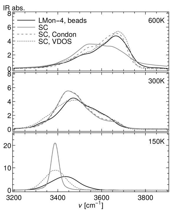
Figure S3: Comparison between LMon-4 spectra and SC line shapes for the OH stretch in HOD:D₂O at different temperatures. The SC lineshape including non-Condon corrections is compared with the vibrational density of states (VDOS) and with the SC lineshape without non-Condon corrections (Condon). Note that at 150K the Condon and non-Condon profiles are indistinguishable.

Appendix D Details of SC calculations

Following Ref. Mukamel (1999), all SC line shapes were calculated using molecular configurations extracted from 10 CMD trajectories of 50 ps. Briefly, for any instantaneous CMD configuration of the HOD:D₂O system, the OH vibrational frequencies and wave functions of both ground and first-excited states were calculated by solving the Schröodinger equation for the corresponding one dimensional oscillator using the Numerov methodNoumerov (1924). The underlying OH potential energy curve was obtained by stretching the OH bond of HOD while keeping the positions of all other atoms fixed. The associated vibrational transition moment ($\mu_{10}$) was calculated within the same computational scheme from the numerical integration of the product of the molecular dipole moment and the appropriate vibrational wave functions. The non-Condon OH line shape for the 1-0 vibrational transition w classical limit was calculated as

$$I^{\text{NC}}(\omega)={{1}\over{2\pi}}\int_{-\infty}^{\infty}dte^{-i\omega t}\langle{\bf\mu}_{10}(0)\cdot{\bf\mu}_{10}(t)e^{i\int_{0}^{t}d\tau\omega_{10}(\tau)}\rangle$$ (8)

where $\mu_{10}$(t) is the vibrational transition moment associated to the transition between the ground and excited state of the OH bond, $\omega_{10}$(t) is the instantaneous vibrational frequency at time t, and the brackets denote a classical equilibrium average. Within the Condon approximation, it is then assumed that the magnitude of the vibrational transition moment is independent of the surrounding environment, which leads to

$$I^{\text{C}}(\omega)\propto\int_{-\infty}^{\infty}dte^{-i\omega t}\langle e^{i\int_{0}^{t}d\tau\omega_{10}(\tau)}\rangle.$$ (9)

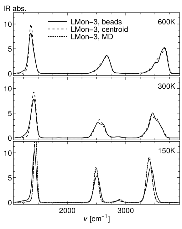
Figure S4: Dependence of LMon-3 on the atomic configuration of HOD in D₂O in the three thermodynamic conditions considered in the manuscript. We compare configurations coming from the beads and from the centroid of PIMD simulations, and from a classical MD simulation. The largest differences are seen for ice at 150K.

The VDOS was obtained simply from making a histogram of the frequencies calculated from all snapshots, but without weighting by the dipole transition moment.

Appendix E LMon dependence on the finite-temperature structure

In the following we study the dependence of the LMon-3 spectra to the use of beads or centroid configurations from PIMD simulations, or configurations coming form a classical MD simulation. The differences are mainly seen at 150K. For OH band, the centroid result is 25 cm^-1 red-shifted with respect to the result for the bead configurations. For the OD band, centroid-derived spectrum has a 10 cm^-1 red-shift if the center of the band is considered. For the bend, centroid has a 18 cm^-1 blue-shift. For ice HOD:D₂O at 150K also the result using classical MD configurations is shown, being quite similar to the one coming from the centroid configurations, which highlights the close-to-classical nature of the centroid in PIMD simulations.

Figure S5: Differences in the spectra obtained from the LMon-3 (dashed) and LMon-4 (full) methods of HOD in D₂O for Ice at 150K. The inset shows a magnification of the combination band of bend and libration that only LMon-4 captures.

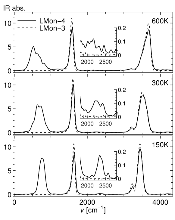
Figure S6: Differences in the spectra obtained from the LMon-3 (dashed) and LMon-4 (full) methods of pure light water. The insets show a magnification of the combination band of bend and libration that only LMon-4 captures.

Appendix F LMon dependence on the quantum subspace size

We here study the differences between a LMon-3 and a LMon-4 (in the ”effective LMon-6” approximation) calculations for the IR spectrum of neat water (H₂O) and HOD in D₂O. First, the intramolecular bands from LMon-4 and LMon-3 are nearly the same. This implies LMon-3 is an effective and accurate method to compute intramolecular bands of the vibrational spectra of condensed-phase matter. Second, LMon-4 is able to capture also intermolecular bands. For H₂O, one of them is a librational band at 400-1000 cm^-1 and the other is a combination band of bend and libration at 2100-2300 cm^-1. For HOD, the librational band is in the range of 400-900 cm^-1 and the combination band appears at around 2000 cm^-1. Expanding the subspace to include a intermolecular mode is therefore an important step. However, LMon-4 is still far from the optimal real LMon-6 (or the ultimate LMon-9), which are much more computationally expensive. We thus believe that the intermolecular bands obtained from separate LMon-4 calculations are considered to be less accurate than the intramolecular bands.

References

- Wang and Bowman (2011) Y. Wang and J. M. Bowman, The Journal of Chemical Physics 134, 154510 (2011).
- Wang and Bowman (2012) Y. Wang and J. M. Bowman, J. Chem. Phys. 136, 144113 (2012).
- Torii (2006) H. Torii, J. Phys. Chem. A 110, 9469 (2006).
- Skinner, Auer, and Lin (2009) J. L. Skinner, B. M. Auer, and Y.-S. Lin, in Advances in Chemical Physics (Wiley-Blackwell, 2009) pp. 59–103.
- Gruenbaum et al. (2013) S. M. Gruenbaum, C. J. Tainter, L. Shi, Y. Ni, and J. L. Skinner, J. Chem. Theory Comput. 9, 3109 (2013).
- Miller (2005) W. H. Miller, Proceedings of the National Academy of Sciences 102, 6660 (2005).
- Liu and Miller (2006) J. Liu and W. H. Miller, J. Chem. Phys. 125, 224104 (2006).
- Liu et al. (2009) J. Liu, W. H. Miller, F. Paesani, W. Zhang, and D. A. Case, J. Chem. Phys. 131, 164509 (2009).
- Cao and Voth (1994) J. Cao and G. A. Voth, J. Chem. Phys. 100, 5106 (1994).
- Jang and Voth (1999) S. Jang and G. A. Voth, J. Chem. Phys. 111, 2371 (1999).
- Craig and Manolopoulos (2004) I. R. Craig and D. E. Manolopoulos, J. Chem. Phys. 121, 3368 (2004).
- Habershon et al. (2013) S. Habershon, D. E. Manolopoulos, T. E. Markland, and T. F. Miller, Annu. Rev. Phys. Chem. 64, 387 (2013).
- Rossi, Ceriotti, and Manolopoulos (2014) M. Rossi, M. Ceriotti, and D. E. Manolopoulos, J. Chem. Phys. 140, 234116 (2014).
- Paesani and Voth (2010) F. Paesani and G. A. Voth, J. Chem. Phys. 132, 014105 (2010).
- Ahlborn et al. (1999) H. Ahlborn, X. Ji, B. Space, and P. B. Moore, The Journal of Chemical Physics 111, 10622 (1999).
- Habershon, Fanourgakis, and Manolopoulos (2008) S. Habershon, G. S. Fanourgakis, and D. E. Manolopoulos, J. Chem. Phys. 129, 074501 (2008).
- Witt et al. (2009) A. Witt, S. D. Ivanov, M. Shiga, H. Forbert, and D. Marx, J. Chem. Phys. 130, 194510 (2009).
- Ivanov et al. (2010) S. D. Ivanov, A. Witt, M. Shiga, and D. Marx, J. Chem. Phys. 132, 031101 (2010).
- Habershon, Markland, and Manolopoulos (2009) S. Habershon, T. E. Markland, and D. E. Manolopoulos, J. Chem. Phys. 131, 024501 (2009).
- Jang, Sinitskiy, and Voth (2014) S. Jang, A. V. Sinitskiy, and G. A. Voth, The Journal of Chemical Physics 140, 154103 (2014).
- Braams and Manolopoulos (2006) B. J. Braams and D. E. Manolopoulos, The Journal of Chemical Physics 125, 124105 (2006).
- Hele and Althorpe (2013) T. J. H. Hele and S. C. Althorpe, The Journal of Chemical Physics 138, 084108 (2013).
- Ceriotti, More, and Manolopoulos (2014) M. Ceriotti, J. More, and D. E. Manolopoulos, Computer Physics Communications 185, 1019 (2014).
- Plimpton (1995) S. Plimpton, Journal of Computational Physics 117, 1 (1995).
- Ceriotti et al. (2010) M. Ceriotti, M. Parrinello, T. E. Markland, and D. E. Manolopoulos, J. Chem. Phys. 133, 124104 (2010).
- Bussi, Donadio, and Parrinello (2007) G. Bussi, D. Donadio, and M. Parrinello, J. Chem. Phys. 126, 014101 (2007).
- Pérez, Tuckerman, and Müser (2009) A. Pérez, M. E. Tuckerman, and M. H. Müser, J. Chem. Phys. 130, 184105 (2009).
- (28) See Supplementary Material Document No xxxxxx for computational details and a discussion of their impact on the results of the different methods.
- Carter, Culik, and Bowman (1997) S. Carter, S. J. Culik, and J. M. Bowman, J. Chem. Phys. 107, 10458 (1997).
- Carter, Bowman, and Handy (1998) S. Carter, J. M. Bowman, and N. C. Handy, Theoretical Chemistry Accounts: Theory Computation, and Modeling (Theoretica Chimica Acta) 100, 191 (1998).
- Bowman, Carter, and Huang (2003) J. M. Bowman, S. Carter, and X. Huang, International Reviews in Physical Chemistry 22, 533 (2003).
- Liu, Wang, and Bowman (2014a) H. Liu, Y. Wang, and J. M. Bowman, The Journal of Physical Chemistry B (2014a), DOI:10.1021/jp5061182.
- Liu, Wang, and Bowman (2014b) H. Liu, Y. Wang, and J. M. Bowman, J. Am. Chem. Soc. 136, 5888 (2014b).
- Mukamel (1999) S. Mukamel, Principles of Nonlinear Optical Spectroscopy (Oxford University Press, 1999).
- Schmidt, Corcelli, and Skinner (2005) J. R. Schmidt, S. A. Corcelli, and J. L. Skinner, J. Chem. Phys. 123, 044513 (2005).
- Bakker and Skinner (2009) H. Bakker and J. Skinner, Chemical reviews 110, 1498 (2009).
- Wang et al. (2011) Y. Wang, X. Huang, B. C. Shepler, B. J. Braams, and J. M. Bowman, J. Chem. Phys. 134, 094509 (2011).
- Paesani, Xantheas, and Voth (2009) F. Paesani, S. S. Xantheas, and G. A. Voth, J. Phys. Chem. B 113, 13118 (2009).
- Choi and Cho (2013) J.-H. Choi and M. Cho, The Journal of Chemical Physics 138, 174108 (2013).
- McQuarrie (2000) D. McQuarrie, Statistical Mechanics, 1st ed. (University Science Books, 2000).
- Hone and Voth (2004) T. D. Hone and G. A. Voth, J. Chem. Phys. 121, 6412 (2004).
- Hoover (1985) W. Hoover, Physical Review A 31, 1695 (1985).
- Nosé (1984) S. Nosé, J. Chem. Phys. 81, 511 (1984).
- Martyna, Klein, and Tuckerman (1992) G. J. Martyna, M. L. Klein, and M. Tuckerman, J. Chem. Phys. 97, 2635 (1992).
- Kinugawa, Moore, and Klein (1997) K. Kinugawa, P. B. Moore, and M. L. Klein, J. Chem. Phys. 106, 1154 (1997).
- Ceriotti, Bussi, and Parrinello (2009) M. Ceriotti, G. Bussi, and M. Parrinello, Phys. Rev. Lett. 102 (2009), 10.1103/physrevlett.102.020601.
- (47) S. Habershon and D. E. Manolopoulos, private communication.
- Noumerov (1924) B. V. Noumerov, Monthly Notices of the Royal Astronomical Society 84, 592 (1924).