Effects of (axial)vector mesons on the chiral phase transition: initial results

Abstract

We investigate the effects of (axial)vector mesons on the chiral phase transition in the framework of an SU(3), (axial)vector meson extended linear sigma model with additional constituent quarks and Polyakov loops. We determine the parameters of the Lagrangian at zero temperature in a hybrid approach, where we treat the mesons at tree-level, while the constituent quarks at 1-loop level. We assume two nonzero scalar condensates and together with the Polyakov-loop variables we determine their temperature dependence according to the 1-loop level field equations.

1 Introduction

Nowadays, investigation of the QCD phase diagram is a very important subject both theoretically and experimentally. Ongoing and upcoming heavy ion experiments such as RHIC, CERN LHC and CBM FAIR explore different regions of the QCD phase space. Since properties of the phase space/boundary is still not settled theoretically/experimentally, it is worth to investigate this subject thoroughly.

Our starting point is the (axial)vector meson extended linear sigma model with additional constituent quarks and Polyakov-loop variables. The previous version of the model, without constituent quarks and Polyakov-loops, was exhaustively analyzed at zero temperature in Parganlija_2013 . The Lagrangian of the model is given by,

$$\mathcal{L} =\mathop{\mathrm{Tr}}[(D_{\mu}\Phi)^{\dagger}(D_{\mu}\Phi)]-m_{0}^{2}\mathop{\mathrm{Tr}}(\Phi^{\dagger}\Phi)-\lambda_{1}[\mathop{\mathrm{Tr}}(\Phi^{\dagger}\Phi)]^{2}-\lambda_{2}\mathop{\mathrm{Tr}}(\Phi^{\dagger}\Phi)^{2}{}$$

$$-\frac{1}{4}\mathop{\mathrm{Tr}}(L_{\mu\nu}^{2}+R_{\mu\nu}^{2})+\mathop{\mathrm{Tr}}\left[\left(\frac{m_{1}^{2}}{2}+\Delta\right)(L_{\mu}^{2}+R_{\mu}^{2})\right]+\mathop{\mathrm{Tr}}[H(\Phi+\Phi^{\dagger})]{}$$

$$+c_{1}(\det\Phi+\det\Phi^{\dagger})+i\frac{g_{2}}{2}(\mathop{\mathrm{Tr}}\{L_{\mu\nu}[L^{\mu},L^{\nu}]\}+\mathop{\mathrm{Tr}}\{R_{\mu\nu}[R^{\mu},R^{\nu}]\}){}$$

$$+\frac{h_{1}}{2}\mathop{\mathrm{Tr}}(\Phi^{\dagger}\Phi)\mathop{\mathrm{Tr}}(L_{\mu}^{2}+R_{\mu}^{2})+h_{2}\mathop{\mathrm{Tr}}[(L_{\mu}\Phi)^{2}+(\Phi R_{\mu})^{2}]+2h_{3}\mathop{\mathrm{Tr}}(L_{\mu}\Phi R^{\mu}\Phi^{\dagger})$$ (1)

$$+g_{3}[\mathop{\mathrm{Tr}}(L_{\mu}L_{\nu}L^{\mu}L^{\nu})+\mathop{\mathrm{Tr}}(R_{\mu}R_{\nu}R^{\mu}R^{\nu})]+g_{4}[\mathop{\mathrm{Tr}}\left(L_{\mu}L^{\mu}L_{\nu}L^{\nu}\right){}$$

$$+\mathop{\mathrm{Tr}}\left(R_{\mu}R^{\mu}R_{\nu}R^{\nu}\right)]+g_{5}\mathop{\mathrm{Tr}}\left(L_{\mu}L^{\mu}\right)\,\mathop{\mathrm{Tr}}\left(R_{\nu}R^{\nu}\right)+g_{6}[\mathop{\mathrm{Tr}}(L_{\mu}L^{\mu})\,\mathop{\mathrm{Tr}}(L_{\nu}L^{\nu}){}$$

$$+\mathop{\mathrm{Tr}}(R_{\mu}R^{\mu})\,\mathop{\mathrm{Tr}}(R_{\nu}R^{\nu})]+\bar{\Psi}i\mbox{$\,/$ $\partial$}\Psi-g_{F}\bar{\Psi}\left(\Phi_{S}+i\gamma_{5}\Phi_{PS}\right)\Psi,{}$$

where $D^{\mu}\Phi=\partial^{\mu}\Phi-ig_{1}(L^{\mu}\Phi-\Phi R^{\mu})-ieA_{e}^{\mu}[T_{3},\Phi],$ $L^{\mu\nu}=\partial^{\mu}L^{\nu}-ieA_{e}^{\mu}[T_{3},L^{\nu}]-\left\{\partial^{\nu}L^{\mu}-ieA_{e}^{\nu}[T_{3},L^{\mu}]\right\},$ and $R^{\mu\nu}=\partial^{\mu}R^{\nu}-ieA_{e}^{\mu}[T_{3},R^{\nu}]-\left\{\partial^{\nu}R^{\mu}-ieA_{e}^{\nu}[T_{3},R^{\mu}]\right\}.$ Here $\Phi$ stands for the scalar and pseudoscalar fields, $L^{\mu}$ and $R^{\mu}$ for the left and right handed vector fields, $\Psi=(u,d,s)^{\text{T}}$ for the constituent quark fields, while $H$ for the external field.

2 Parametrization

In order to go to finite temperature/chemical potential, parameters of the Lagrangian have to be determined, which is done at $T=\mu=0$. For this we calculate tree-level masses and decay widths of the model and compare them with the experimental data taken from the PDG PDG . For the comparison we use a $\chi^{2}$ minimalization method MINUIT to fit our parameters (for more details see Parganlija_2013 ). It is important to note that in the present work we also included in the scalar and pseudoscalar masses the contributions coming from the fermion vacuum fluctuations by adapting the method of Chatterjee:2011jd .

We have $14$ unknown parameters, namely $m_{0}$, $\lambda_{1}$, $\lambda_{2}$, $c_{1}$, $m_{1}$, $g_{1}$, $g_{2}$, $h_{1}$, $h_{2}$, $h_{3}$, $\delta_{S}$, $\Phi_{N}$, $\Phi_{S}$, and $g_{F}$. Here $g_{F}$ is the coupling of the additionally introduced Yukawa term, which can be determined from the constituent quark masses through the equations $m_{u/d}=g_{F}\phi_{N}/2$, $m_{s}=g_{F}\phi_{s}/\sqrt{2}$.

It is worth to note that if we do not consider the very uncertain scalar-isoscalar sector $m_{0}$, and $\lambda_{1}$ always appear in the same combination $C_{1}=m_{0}^{2}+\lambda_{1}\left(\phi_{N}^{2}+\phi_{S}^{2}\right)$ in all the expressions, thus we can not determine them separately. Additionally a similar combination appears for $m_{1}$ and $h_{1}$ in the vector sector as $C_{2}=m_{1}^{2}+\frac{h_{1}}{2}\left(\phi_{N}^{2}+\phi_{S}^{2}\right)$ (see details in Parganlija_2013 ). The parameter values are given in Table 1.

Table 1: Parameters determined by $\chi^{2}$ minimalization

Parameter	Value	Parameter	Value
$\phi_{N}$ [GeV]	$0.1622$	$h_{2}$	$11.6586$
$\phi_{S}$ [GeV]	$0.1262$	$h_{3}$	$4.7028$
$C_{1}$ [GeV2]	$-0.7537$	$\delta_{S}$ [GeV2]	$0.1534$
$C_{2}$ [GeV2]	$0.3953$	$c_{1}$ [GeV]	$1.12$
$\lambda_{1}$	undetermined	$g_{1}$	$-5.8943$
$\lambda_{2}$	$65.3221$	$g_{2}$	$-2.9960$
$h_{1}$	undetermined	$g_{F}$	$4.9429$

Since $\lambda_{1}$ is undetermined it can be tuned to change the $f_{0}^{L}$ (a.k.a. $\sigma$) mass, which has, as we will see, a huge effect on the thermal properties of the model.

3 Field equations

In our approach we have four order parameters, which are the $\phi_{N}$ non-strange and $\phi_{S}$ strange condensates, and the $\Phi$ and $\bar{\Phi}$ Polyakov-loop variables. The condensates arise due to the spontaneous symmetry breaking, while the Polyakov-loop variables naturally emerge in mean field approximation, if one calculates free fermion grand canonical potential on a constant gluon background. The effect of fermions propagating on a constant gluon background in the temporal direction formally amounts to the appearance of imaginary color dependent chemical potentials (for details see Marko_2010 ; Korthals_1999 ).

At finite temperature/baryochemical potential we can set up four coupled field equations for the four fields, which are just the requirements that the first derivatives of the grand canonical potential according to the fields must vanish. As a first approximation we apply a hybrid approach in which we only consider vacuum and thermal fluctuations for the fermions, but not for the bosons. Within this simplified treatment the equations are the following

$$-\frac{d}{d\Phi}\left(\frac{U(\Phi,\bar{\Phi})}{T^{4}}\right)+\frac{2N_{c}}{T^{3}}\sum_{q=u,d,s}\int\frac{d^{3}{\bf p}}{(2\pi)^{3}}\left(\frac{e^{-\beta E_{q}^{-}(p)}}{g_{q}^{-}(p)}+\frac{e^{-2\beta E_{q}^{+}(p)}}{g_{q}^{+}(p)}\right) =0,$$ (2)

$$-\frac{d}{d\bar{\Phi}}\left(\frac{U(\Phi,\bar{\Phi})}{T^{4}}\right)+\frac{2N_{c}}{T^{3}}\sum_{q=u,d,s}\int\frac{d^{3}{\bf p}}{(2\pi)^{3}}\left(\frac{e^{-\beta E_{q}^{+}(p)}}{g_{q}^{+}(p)}+\frac{e^{-2\beta E_{q}^{-}(p)}}{g_{q}^{-}(p)}\right) =0,$$ (3)

$$m_{0}^{2}\phi_{N}+\left(\lambda_{1}+\frac{1}{2}\lambda_{2}\right)\phi_{N}^{3}+\lambda_{1}\phi_{N}\phi_{S}^{2}-h_{N}+\frac{g_{F}}{2}N_{c}\left(\langle u{\bar{u}}\rangle_{{}_{T}}+\langle d{\bar{d}}\rangle_{{}_{T}}\right) =0,$$ (4)

$$m_{0}^{2}\phi_{S}+\left(\lambda_{1}+\lambda_{2}\right)\phi_{S}^{3}+\lambda_{1}\phi_{N}^{2}\phi_{S}-h_{S}+\frac{g_{F}}{\sqrt{2}}N_{c}\langle s{\bar{s}}\rangle_{{}_{T}} =0,$$ (5)

where

$$g_{q}^{+}(p) =1+3\left(\bar{\Phi}+\Phi e^{-\beta E_{q}^{+}(p)}\right)e^{-\beta E_{q}^{+}(p)}+e^{-3\beta E_{q}^{+}(p)},$$

$$g_{q}^{-}(p) =1+3\left(\Phi+\bar{\Phi}e^{-\beta E_{q}^{-}(p)}\right)e^{-\beta E_{q}^{-}(p)}+e^{-3\beta E_{q}^{-}(p)},$$

$$E_{q}^{\pm}(p)= E_{q}(p)\mp\mu_{B}/3,\;E_{u/d}(p)=\sqrt{p^{2}+m_{u/d}^{2}},\;E_{s}(p)=\sqrt{p^{2}+m_{s}^{2}},$$

and

$$\langle q{\bar{q}}\rangle_{{}_{T}} =-4m_{q}\int\frac{d^{3}{\bf p}}{(2\pi)^{3}}\frac{1}{2E_{q}(p)}\left(1-f^{-}_{\Phi}(E_{q}(p))-f^{+}_{\Phi}(E_{q}(p))\right),$$ (6)

with the modified distribution functions

$$f^{+}_{\Phi}(E_{p}) =\frac{\left(\bar{\Phi}+2\Phi e^{-\beta\left(E_{p}-\mu_{q}\right)}\right)e^{-\beta\left(E_{p}-\mu_{q}\right)}+e^{-3\beta\left(E_{p}-\mu_{q}\right)}}{1+3\left(\bar{\Phi}+\Phi e^{-\beta\left(E_{p}-\mu_{q}\right)}\right)e^{-\beta\left(E_{p}-\mu_{q}\right)}+e^{-3\beta\left(E_{p}-\mu_{q}\right)}},{}$$

$$f^{-}_{\Phi}(E_{p}) =\frac{\left(\Phi+2\bar{\Phi}e^{-\beta\left(E_{p}+\mu_{q}\right)}\right)e^{-\beta\left(E_{p}+\mu_{q}\right)}+e^{-3\beta\left(E_{p}+\mu_{q}\right)}}{1+3\left(\Phi+\bar{\Phi}e^{-\beta\left(E_{p}+\mu_{q}\right)}\right)e^{-\beta\left(E_{p}+\mu_{q}\right)}+e^{-3\beta\left(E_{p}+\mu_{q}\right)}}.{}$$

4 Results

Solving Eqs. 2-5 we get the temperature dependence of the order parameters, which can be seen in Fig. 2.

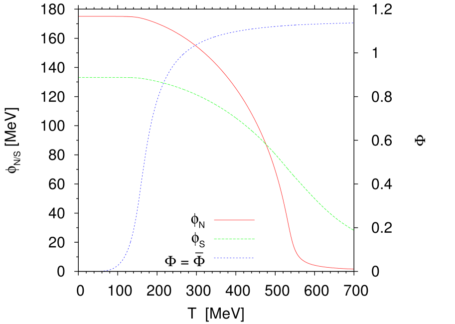
Figure 1: Temperature dependence of the order parameters with $m_{\sigma}=1.3$ GeV

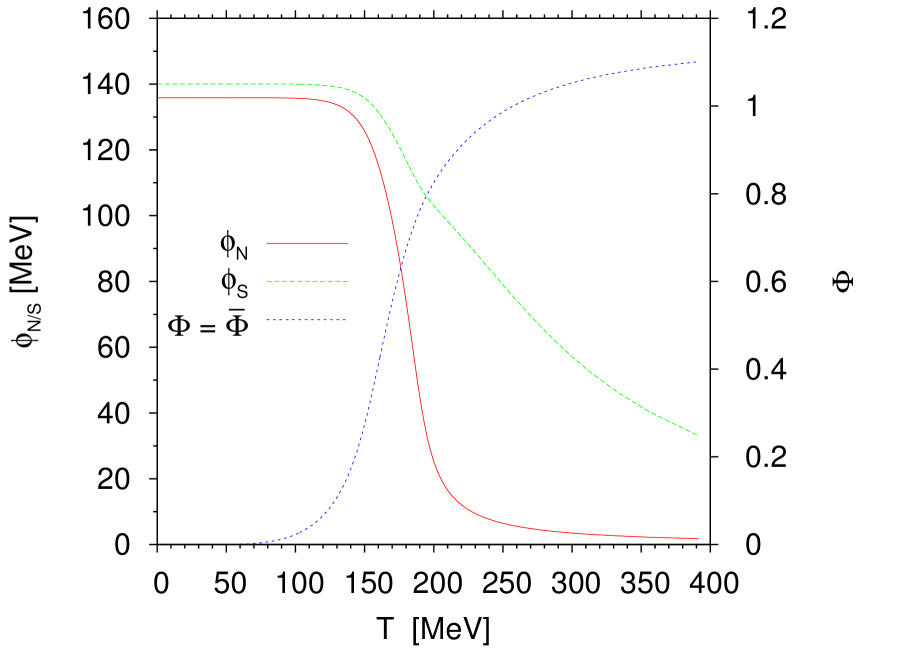
Figure 2: Temperature dependence of the order parameters with $m_{\sigma}=0.4$ GeV

In Parganlija_2013 it was shown that the $q\bar{q}$ scalar nonet most probably contains $f_{0}$’s with masses higher than $1$ GeV. If we set $\lambda_{1}=0$ we get $m_{f_{0}^{L}}=1.3$ GeV, which is in agreement with Parganlija_2013 . However in this case we get a very high pseudocritical temperature, $T_{c}\approx 550$ MeV, for $\phi_{N}$, which is much larger than earlier results (e.g. on lattice $T_{c}\approx 150$ MeV Aoki ). Now, if we tune $\lambda_{1}$ to get $m_{f_{0}^{L}}400$ MeV (which corresponds to the physical particle $f_{0}(500)$), than $T_{c}$ goes down to $150-200$ MeV, which can be seen in Fig. 2. This suggests that in order to get a good pseudocritical temperature we would need a scalar-isoscalar particle with low mass ($\sim 400$ MeV), which is most probably not a $q\bar{q}$ state according to Parganlija_2013 .

Authors were supported by the Hungarian OTKA fund K109462.

References

• (1) D. Parganlija, P. Kovacs, G. Wolf, F. Giacosa and D. H. Rischke, Phys. Rev. D 87, 014011 (2013).
• (2) J. Beringer et al. (Particle Data Group), Phys. Rev. D86, 010001 (2012).
• (3) F. James and M. Roos, Comput. Phys. Commun. 10, 343 (1975).
• (4) S. Chatterjee and K. A. Mohan, Phys. Rev. D 85, 074018 (2012).
• (5) G. Markó and Zs. Szép, Phys. Rev. D 82, 065021 (2010).
• (6) C. P. Korthals Altes, R. D. Pisarski and A. Sinkovics, Phys. Rev. D 61, 056007 (2000).
• (7) Y. Aoki et al., PLB 643, 46 (2006).