Very Large-Scale Singular Value Decomposition Using Tensor Train Networks

Abstract

We propose new algorithms for singular value decomposition (SVD) of very large-scale matrices based on a low-rank tensor approximation technique called the tensor train (TT) format. The proposed algorithms can compute several dominant singular values and corresponding singular vectors for large-scale structured matrices given in a TT format. The computational complexity of the proposed methods scales logarithmically with the matrix size under the assumption that both the matrix and the singular vectors admit low-rank TT decompositions. The proposed methods, which are called the alternating least squares for SVD (ALS-SVD) and modified alternating least squares for SVD (MALS-SVD), compute the left and right singular vectors approximately through block TT decompositions. The very large-scale optimization problem is reduced to sequential small-scale optimization problems, and each core tensor of the block TT decompositions can be updated by applying any standard optimization methods. The optimal ranks of the block TT decompositions are determined adaptively during iteration process, so that we can achieve high approximation accuracy. Extensive numerical simulations are conducted for several types of TT-structured matrices such as Hilbert matrix, Toeplitz matrix, random matrix with prescribed singular values, and tridiagonal matrix. The simulation results demonstrate the effectiveness of the proposed methods compared with standard SVD algorithms and TT-based algorithms developed for symmetric eigenvalue decomposition.

KEY WORDS: curse-of-dimensionality, low-rank tensor approximation, matrix factorization, symmetric eigenvalue decomposition, singular value decomposition, tensor decomposition, tensor network, matrix product operator, Hankel matrix, Toeplitz matrix, tridiagonal matrix

1 Introduction

The singular value decomposition (SVD) is one of the most important matrix factorization techniques in numerical analysis. The SVD can be used for the best low-rank approximation for matrices, computation of pseudo-inverses of matrices, solution of unconstrained linear least squares problems, principal component analysis, cannonical correlation analysis, and estimation of ranks and condition numbers of matrices, just to name a few. It has a wide range of applications in image processing, signal processing, immunology, molecular biology, information retrieval, systems biology, computational finance, and so on [44].

In this paper, we propose two algorithms for computing $K$ dominant singular values and corresponding singular vectors of structured very large-scale matrices. The $K$ dominant singular values/vectors can be computed by solving the following trace maximization problem: given $\mathbf{A}\in\mathbb{R}^{P\times Q}$,

$$\begin{split}\mathop{\text{maximize}}_{\mathbf{U},\mathbf{V}}&\qquad\text{trace}\left(\mathbf{U}^{\mathrm{T}}\mathbf{A}\mathbf{V}\right)\\ \text{subject to}&\qquad\mathbf{U}^{\mathrm{T}}\mathbf{U}=\mathbf{V}^{\mathrm{T}}\mathbf{V}=\mathbf{I}_{K}.\end{split}$$ (1)

This can be derived based on the fact that the SVD of $\mathbf{A}$ is closely related to the eigenvalue decomposition (EVD) of the symmetric matrix $\begin{bmatrix}\mathbf{0}&\mathbf{A}\\ \mathbf{A}^{\mathrm{T}}&\mathbf{0}\end{bmatrix}$ [6, Theorem 3.3], and the Ky Fan trace min/max principles [12, Theorem 1]. See Appendix A for more detail. Standard algorithms for computing the SVD of a $P\times Q$ matrix with $P\geq Q$ cost $\mathcal{O}(PQ^{2})$ for computing full SVD [4, Table 3], and $\mathcal{O}(PQK)$ for computing $K$ dominant singular values [31, Section 2.4]. However, in case that $P$ and $Q$ are exponentially growing, e.g., $P=Q=I^{N}$ for some fixed $I$, the computational and storage complexities also grow exponentially with $N$. In order to avoid the “curse-of-dimensionality”, the Monte-Carlo algorithm [13] was suggested but its accuracy is not high enough.

The basic idea behind the proposed algorithms is to reshape (or tensorize) matrices and vectors into high-order tensors and compress them by applying a low-rank tensor approximation technique [15]. Once the matrices and vectors are represented in low-rank tensor formats such as the tensor train (TT) [34, 37] or hierarchical Tucker (HT) [14, 17] decompositions, all the basic numerical operations such as the matrix-by-vector multiplication are performed based on the low-rank tensor formats with feasible computational complexities growing only linearly in $N$ [14, 34].

On the other hand, traditional low-rank tensor approximation techniques such as the CANDECOMP/PARAFAC (CP) and Tucker decompositions also compress high-order tensors into low-parametric tensor formats [24]. Although the CP and Tucker decompositions have a wide range of applications in chemometrics, signal processing, neuroscience, data mining, image processing, and numerical analysis [24], they have their own limitations. The Tucker decomposition cannot avoid the curse-of-dimensionality, which prohibits its application to the tensorized large-scale data matrices [15]. The CP decomposition does not suffer from the curse-of-dimensionality, but there does not exist a reliable and stable algorithm for best low-rank approximation due to the lack of closedness of the set of tensors of bounded tensor ranks [7].

In this paper, we focus on the TT decomposition, which is one of the most simplest tensor network formats [10]. The TT and HT decompositions can avoid the curse-of-dimensionality by low-rank approximation, and possess the closedness property [10, 11]. For numerical analysis, basic numerical operations such as addition and matrix-by-vector multiplication based on low-rank TT formats usually lead to TT-rank growth, so an efficient rank-truncation should be followed. Efficient rank-truncation algorithms for the TT and HT decompositions were developed in [14, 34].

The computation of extremal eigen/singular values and the corresponding eigen/singular vectors are usually obtained by solving an optimization problem such as the one in (1) or by maximizing/minimizing the Rayleigh quotient [6]. In order to solve large-scale optimization problems based on the TT decomposition, several different types of optimization algorithms have been suggested in the literature.

First, existing iterative methods can be combined with truncation of the TT format [20, 28, 33]. For example, for computing several extremal eigenvalues of symmetric matrices, conjugate-gradient type iterative algorithms are combined with truncation for minimizing the (block) Rayleigh quotient in [28, 33]. In the case that a few eigenvectors should be computed simultaneously, the block of orthonormal vectors can be efficiently represented in block TT format [28]. However, the whole matrix-by-vector multiplication causes all the TT-ranks to grow at the same time, which leads to a very high computational cost in the subsequent truncation step.

Second, alternating least squares (ALS) type algorithms reduce the given large optimization problem into sequential relatively small optimization problems, for which any standard optimization algorithm can be applied. The ALS algorithm developed in [19] is easy to implement and each iteration is relatively fast. But the TT-ranks should be predefined in advance and cannot be changed during iteration. The modified alternating least squares (MALS) algorithm, or equivalently density matrix renormalization group (DMRG) method [19, 22, 40] can adaptively determine the TT-ranks by merging two core tensors into one bigger core tensor and separating it by using the truncated SVD. The MALS shows a fast convergence in many numerical simulations. However, the reduced small optimization problem is solved over the merged bigger core tensor, which increases the computational and storage costs considerably in some cases. Dolgov et al. [8] developed an alternative ALS type method based on block TT format, where the mode corresponding to the number $K$ of orthonormal vectors is allowed to move to the next core tensor via the truncated SVD. This procedure can determine the TT-ranks adaptively if $K>1$ for the block TT format. Dolgov and Savostyanov [9] and Kressner et al. [25] further developed an ALS type method which adds rank-adaptivity to the block TT-based ALS method even if $K=1$.

In this paper, we propose the ALS and MALS type algorithms for computing $K$ dominant singular values of matrices which are not necessarily symmetric. The ALS algorithm based on block TT format was originally developed for block Rayleigh quotient minimization for symmetric matrices [8]. The MALS algorithm was also developed for Rayleigh quotient minimization for symmetric matrices [19, 22, 40]. We show that the $K$ dominant singular values can be efficiently computed by solving the maximization problem (1). We compare the proposed algorithms with other block TT-based algorithms which were originally developed for computing eigenvalues of symmetric matrices, by simulated experiments and a theoretical analysis of computational complexities.

Moreover, we present extensive numerical experiments for various types of structured matrices such as Hilbert matrix, Toeplitz matrix, random matrix with prescribed singular values, and tridiagonal matrix. We compare the performances of several different SVD algorithms, and we present the relationship between TT-ranks and approximation accuracy based on the experimental results. We show that the proposed block TT-based algorithms can achieve very high accuracy by adaptively determining the TT-ranks. It is shown that the proposed algorithms can solve very large-scale optimization problems for matrices of as large sizes as $2^{50}\times 2^{50}$ on desktop computers.

The paper is organized as follows. In Section 2, notations for tensor operations and TT formats are described. In Section 3, the proposed SVD algorithms based on block TT format is presented. Their computational complexities are analyzed and computational considerations are discussed. In Section 4, extensive experimental results are presented for analysis and comparison of performances of SVD algorithms for several types of structured matrices. Conclusion and discussions are given in Section 5.

2 Tensor Train Formats

2.1 Notations

We refer to [3, 24, 29] for notations for tensors and multilinear operations. Scalars, vectors, and matrices are denoted by lowercase, lowercase bold, and uppercase bold letters as $x$, $\mathbf{x}$, and $\mathbf{X}$, respectively. An $N$th order tensor $\underline{\mathbf{X}}$ is a multi-way array of size $I_{1}\times I_{2}\times\cdots\times I_{N}$, where $I_{n}$ is the size of the $n$th dimension or mode. A vector is a 1st order tensor and a matrix is a 2nd order tensor. The $(i_{1},i_{2},\ldots,i_{N})$th entry of $\underline{\mathbf{X}}\in\mathbb{R}^{I_{1}\times I_{2}\times\cdots\times I_{N}}$ is denoted by either $x_{i_{1},i_{2},\ldots,i_{N}}$ or $\underline{\mathbf{X}}(i_{1},i_{2},\ldots,i_{N})$. Let $(i_{1},i_{2},\ldots,i_{N})$ denote the multi-index defined by

$$(i_{1},i_{2},\ldots,i_{N})=i_{1}+(i_{2}-1)I_{1}+\cdots+(i_{N}-1)I_{1}I_{2}\cdots I_{N-1}.$$ (2)

The vectorization of a tensor $\underline{\mathbf{X}}\in\mathbb{R}^{I_{1}\times I_{2}\times\cdots\times I_{N}}$ is denoted by

$$\text{vec}(\underline{\mathbf{X}})\in\mathbb{R}^{I_{1}I_{2}\cdots I_{N}},$$ (3)

and each entry of $\text{vec}(\underline{\mathbf{X}})$ is associated with each entry of $\underline{\mathbf{X}}$ by

$$\left(\text{vec}(\underline{\mathbf{X}})\right)_{(i_{1},i_{2},\ldots,i_{N})}=\underline{\mathbf{X}}(i_{1},i_{2},\ldots,i_{N})$$ (4)

like in MATLAB. For each $n=1,2,\ldots,N$, the mode-$n$ matricization of a tensor $\underline{\mathbf{X}}\in\mathbb{R}^{I_{1}\times\cdots\times I_{N}}$ is defined by

$$\mathbf{X}_{(n)}\in\mathbb{R}^{I_{n}\times I_{1}\cdots I_{n-1}I_{n+1}\cdots I_{N}}$$ (5)

with entries

$$\left(\mathbf{X}_{(n)}\right)_{i_{n},(i_{1},\ldots,i_{n-1},i_{n+1},\ldots,i_{N})}=\underline{\mathbf{X}}(i_{1},i_{2},\ldots,i_{N}).$$ (6)

Tensorization is the reverse process of the vectorization, by which large-scale vectors and matrices are reshaped into higher-order tensors. For instance, a vector of length $I_{1}I_{2}\cdots I_{N}$ can be reshaped into a tensor of size $I_{1}\times I_{2}\times\cdots\times I_{N}$, and a matrix of size $I_{1}I_{2}\cdots I_{N}\times J_{1}J_{2}\cdots J_{N}$ can be reshaped into a tensor of size $I_{1}\times I_{2}\times\cdots\times I_{N}\times J_{1}\times J_{2}\times\cdots\times J_{N}$.

The mode-$n$ product of a tensor $\underline{\mathbf{A}}\in\mathbb{R}^{I_{1}\times\cdots\times I_{N}}$ and a matrix $\mathbf{B}\in\mathbb{R}^{J\times I_{n}}$ is defined by

$$\underline{\mathbf{C}}=\underline{\mathbf{A}}\times_{n}\mathbf{B}\in\mathbb{R}^{I_{1}\times\cdots\times I_{n-1}\times J\times I_{n+1}\times\cdots\times I_{N}}$$ (7)

with entries

$$c_{i_{1},\ldots,i_{n-1},j,i_{n+1},\ldots,i_{N}}=\sum_{i_{n}=1}^{I_{N}}a_{i_{1},\ldots,i_{N}}b_{j,i_{n}}.$$ (8)

The mode-$(M,1)$ contracted product of tensors $\underline{\mathbf{A}}\in\mathbb{R}^{I_{1}\times I_{2}\times\cdots\times I_{M}}$ and $\underline{\mathbf{B}}\in\mathbb{R}^{I_{M}\times J_{2}\times J_{3}\times\cdots\times J_{N}}$ is defined by

$$\underline{\mathbf{C}}=\underline{\mathbf{A}}\bullet\underline{\mathbf{B}}\in\mathbb{R}^{I_{1}\times I_{2}\times\cdots\times I_{M-1}\times J_{2}\times J_{3}\times\cdots\times J_{N}}$$ (9)

with entries

$$c_{i_{1},i_{2},\ldots,i_{M-1},j_{2},j_{3},\ldots,j_{N}}=\sum_{i_{M}=1}^{I_{M}}a_{i_{1},i_{2},\ldots,i_{M}}b_{i_{M},j_{2},j_{3},\ldots,j_{N}}.$$ (10)

The mode-$(M,1)$ contracted product is a natural generalization of the matrix-by-matrix multiplication.

Tensors and tensor operations are often represented as tensor network diagrams for illustrating the underlying principles of algorithms and tensor operations [19]. Figure 1 shows examples of the tensor network diagrams for tensors and tensor operations. In Figure 1(a), a tensor is represented by a node with as many edges as its order. In Figure 1(b), the mode-$(3,1)$ contracted product is represented as the link between two nodes. Figure 1(c) represents the tensorization process of a vector into a 3rd order tensor. Figure 1(d) represents a singular value decomposition of an $I\times J$ matrix into the product $\mathbf{U\Sigma V}^{\mathrm{T}}$. The matrices $\mathbf{U}$ and $\mathbf{V}$ of orthonormal column vectors are represented by half-filled circles, and the diagonal matrix $\mathbf{\Sigma}$ is represented by a circle with slash.

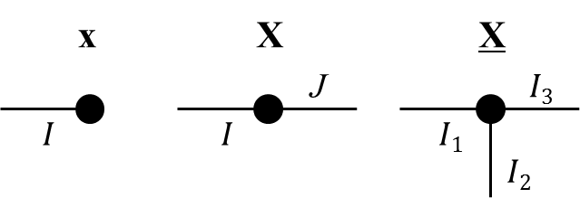
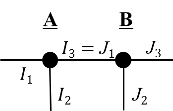
(a)	(b)
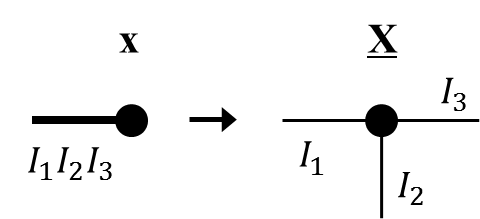
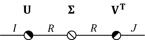
(c)	(d)

Figure 1: Tensor network diagrams for (a) a vector, a matrix, a 3rd order tensor, (b) the mode-$(3,1)$ contracted product of two 3rd order tensors, (c) the tensorization of a vector, and (d) singular value decomposition of an $I\times J$ matrix

2.2 Tensor Train Format

A tensor $\underline{\mathbf{X}}\in\mathbb{R}^{I_{1}\times I_{2}\times\cdots\times I_{N}}$ is in TT format if it is represented by

$$\underline{\mathbf{X}}=\underline{\mathbf{X}}^{(1)}\bullet\underline{\mathbf{X}}^{(2)}\bullet\cdots\bullet\underline{\mathbf{X}}^{(N-1)}\bullet\underline{\mathbf{X}}^{(N)},$$ (11)

where $\underline{\mathbf{X}}^{(n)}\in\mathbb{R}^{R_{n-1}\times I_{n}\times R_{n}},n=1,2,\ldots,N$, are 3rd order core tensors which are called as TT-cores, and $R_{1},R_{2},\ldots,R_{N-1}$ are called as TT-ranks. It is assumed that $R_{0}=R_{N}=1$.

Figure 2 shows the tensor network diagram for an $N$th order tensor in TT format. Each of the core tensors is represented as a third order tensor except the first and the last TT-cores, which are matrices.

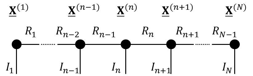
Figure 2: Tensor network diagram for an $N$th order tensor in TT format

The TT format is often called the matrix product states (MPS) with open boundary conditions in quantum physics community because each entry of $\underline{\mathbf{X}}$ in (11) can be written by the products of matrices as

$$x_{i_{1},i_{2},\ldots,i_{N}}=\mathbf{X}^{(1)}_{i_{1}}\mathbf{X}^{(2)}_{i_{2}}\cdots\mathbf{X}^{(N)}_{i_{N}},$$ (12)

where $\mathbf{X}^{(n)}_{i_{n}}=\underline{\mathbf{X}}^{(n)}(:,i_{n},:)\in\mathbb{R}^{R_{n-1}\times R_{n}}$ are the slice matrices of $\underline{\mathbf{X}}^{(n)}$. Note that $\mathbf{X}^{(1)}_{i_{1}}\in\mathbb{R}^{1\times R_{1}}$ and $\mathbf{X}^{(N)}_{i_{N}}\in\mathbb{R}^{R_{N}\times 1}$ are row and column vectors, respectively. Each entry of $\underline{\mathbf{X}}$ can also be written by sums of scalar products

$$x_{i_{1},i_{2},\ldots,i_{N}}=\sum_{r_{1}=1}^{R_{1}}\sum_{r_{2}=1}^{R_{2}}\cdots\sum_{r_{N-1}=1}^{R_{N-1}}x^{(1)}_{1,i_{1},r_{1}}x^{(2)}_{r_{1},i_{2},r_{2}}\cdots x^{(N)}_{r_{N-1},i_{N},1},$$ (13)

where $x^{(n)}_{r_{n-1},i_{n},r_{n}}=\underline{\mathbf{X}}^{(n)}(r_{n-1},i_{n},r_{n})\in\mathbb{R}$ is the entry of the $n$th TT-core $\underline{\mathbf{X}}^{(n)}$. The tensor $\underline{\mathbf{X}}$ in TT format can also be written by the outer products of the fibers (or column vectors) as

$$\underline{\mathbf{X}}=\sum_{r_{1}=1}^{R_{1}}\sum_{r_{2}=1}^{R_{2}}\cdots\sum_{r_{N-1}=1}^{R_{N-1}}\mathbf{x}^{(1)}_{1,r_{1}}\circ\mathbf{x}^{(2)}_{r_{1},r_{2}}\circ\cdots\circ\mathbf{x}^{(N)}_{r_{N-1},1},$$ (14)

where $\circ$ is the outer product and $\mathbf{x}^{(n)}_{r_{n-1},r_{n}}=\underline{\mathbf{X}}^{(n)}(r_{n-1},:,r_{n})\in\mathbb{R}^{I_{n}}$ is the mode-$2$ fiber of the $n$th TT-core $\underline{\mathbf{X}}^{(n)}$.

The storage cost for a TT format is $\mathcal{O}(NIR^{2})$, where $I=\max(I_{n})$ and $R=\max(R_{n})$, that is linear with the order $N$. Any tensor can be represented exactly or approximately in TT format by using the TT-SVD algorithm in [34]. Moreover, basic numerical operations such as the matrix-by-vector multiplication can be performed in time linear with $N$ under the assumption that the TT-ranks are bounded [34].

2.3 Tensor Train Formats for Vectors and Matrices

Any large-scale vector or matrix can also be represented in TT format. We suppose that a vector $\mathbf{x}\in\mathbb{R}^{I_{1}I_{2}\cdots I_{N}}$ is tensorized into a tensor $\underline{\mathbf{X}}\in\mathbb{R}^{I_{1}\times I_{2}\times\cdots\times I_{N}}$ and consider the TT format (11) as the TT representation of $\mathbf{x}=\text{vec}(\underline{\mathbf{X}})$.

Similarly, a matrix $\mathbf{A}\in\mathbb{R}^{I_{1}I_{2}\cdots I_{N}\times J_{1}J_{2}\cdots J_{N}}$ is considered to be tensorized and permuted into a tensor $\underline{\mathbf{A}}\in\mathbb{R}^{I_{1}\times J_{1}\times I_{2}\times J_{2}\times\cdots\times I_{N}\times J_{N}}$. Then, as in (11), the tensor $\underline{\mathbf{A}}$ is represented in TT format as contracted products of TT-cores

$$\underline{\mathbf{A}}=\underline{\mathbf{A}}^{(1)}\bullet\underline{\mathbf{A}}^{(2)}\bullet\cdots\bullet\underline{\mathbf{A}}^{(N)},$$ (15)

where $\underline{\mathbf{A}}^{(n)}\in\mathbb{R}^{R^{A}_{n-1}\times I_{n}\times J_{n}\times R^{A}_{n}},n=1,2,\ldots,N$, are 4th order TT-cores with TT-ranks $R^{A}_{1},R^{A}_{2},\ldots,R^{A}_{N-1}$. We suppose that $R^{A}_{0}=R^{A}_{N}=1$. The entries of $\underline{\mathbf{A}}$ can also be represented in TT format by the products of slice matrices

$$a_{i_{1},j_{1},i_{2},j_{2},\ldots,i_{N},j_{N}}=\mathbf{A}^{(1)}_{i_{1},j_{1}}\mathbf{A}^{(2)}_{i_{2},j_{2}}\cdots\mathbf{A}^{(N)}_{i_{N},j_{N}},$$ (16)

where $\mathbf{A}^{(n)}_{i_{n},j_{n}}=\underline{\mathbf{A}}^{(n)}(:,i_{n},j_{n},:)\in\mathbb{R}^{R^{A}_{n-1}\times R^{A}_{n}}$ is the slice of the $n$th TT-core $\underline{\mathbf{A}}^{(n)}$.

In this paper, we call the TT formats (11) and (15) as the vector TT and matrix TT formats, respectively. Note that if the indices $i_{n}$ and $j_{n}$ are joined as $k_{n}=(i_{n},j_{n})$ in (16), then the matrix TT format is reduced to the vector TT format. Figure 3 shows a tensor network representing a matrix of size $I_{1}I_{2}\cdots I_{N}\times J_{1}J_{2}\cdots J_{N}$ in matrix TT format. Each of the TT-cores is represented as a 4th order tensor except the first and the last core tensor.

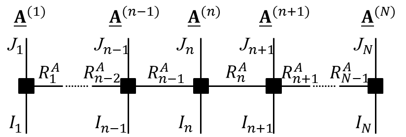
Figure 3: Tensor network diagram for a matrix of size $I_{1}I_{2}\cdots I_{N}\times J_{1}J_{2}\cdots J_{N}$ in matrix TT format

2.4 Block TT Format

A group of several vectors can be represented in block TT format as follows. Let $\mathbf{U}=\left[\mathbf{u}_{1},\mathbf{u}_{2},\ldots,\mathbf{u}_{K}\right]\in\mathbb{R}^{I_{1}I_{2}\cdots I_{N}\times K}$ denote a matrix with $K$ column vectors. Suppose that the matrix $\mathbf{U}$ is tensorized and permuted into a tensor $\underline{\mathbf{U}}\in\mathbb{R}^{I_{1}\times I_{2}\times\cdots\times I_{n-1}\times K\times I_{n}\times\cdots\times I_{N}}$, where the mode of the size $K$ is located between the modes of the sizes $I_{n-1}$ and $I_{n}$ for a fixed $n$. In block TT format, the tensor $\underline{\mathbf{U}}$ is represented as contracted products of TT-cores

$$\underline{\mathbf{U}}=\underline{\mathbf{U}}^{(1)}\bullet\underline{\mathbf{U}}^{(2)}\bullet\cdots\bullet\underline{\mathbf{U}}^{(N)},$$ (17)

where the $n$th TT-core $\underline{\mathbf{U}}^{(n)}\in\mathbb{R}^{R^{U}_{n-1}\times K\times I_{n}\times R^{U}_{n}}$ is a 4th order tensor and the other TT-cores $\underline{\mathbf{U}}^{(m)}\in\mathbb{R}^{R^{U}_{m-1}\times I_{m}\times R^{U}_{m}},m\neq n,$ are 3rd order tensors. We suppose that $R^{U}_{0}=R^{U}_{N}=1$. Each entry of $\underline{\mathbf{U}}$ can be expressed by the products of slice matrices

$$u_{i_{1},i_{2},\ldots,i_{n-1},k,i_{n},\ldots,i_{N}}=\mathbf{U}^{(1)}_{i_{1}}\mathbf{U}^{(2)}_{i_{2}}\cdots\mathbf{U}^{(n-1)}_{i_{n-1}}\mathbf{U}^{(n)}_{k,i_{n}}\mathbf{U}^{(n+1)}_{i_{n+1}}\cdots\mathbf{U}^{(N)}_{i_{N}},$$ (18)

where $\mathbf{U}^{(m)}_{i_{m}}\in\mathbb{R}^{R^{U}_{m-1}\times R^{U}_{m}},m\neq n,$ and $\mathbf{U}^{(n)}_{k,i_{n}}\in\mathbb{R}^{R^{U}_{n-1}\times R^{U}_{n}}$ are the slice matrices of the $m$th and $n$th TT-cores. We note that for a fixed $k\in\{1,2,\ldots,K\}$, the subtensor $\underline{\mathbf{U}}^{(n)}(:,k,:,:)\in\mathbb{R}^{R_{n-1}\times I_{n}\times R_{n}}$ of the $n$th TT-core is of order 3. Hence, the $k$th column vector $\mathbf{u}_{k}$ is in the vector TT format with TT-ranks bounded by $(R^{U}_{1},\ldots,R^{U}_{N-1})$.

In this paper, we call the block TT format (17) as the block-$n$ TT format, termed by [25], in order to distinguish between different permutations of modes. Figure 4 shows a tensor network representing a matrix $\mathbf{U}\in\mathbb{R}^{I_{1}I_{2}\cdots I_{N}\times K}$ in block-$n$ TT format. We can see that the mode of the size $K$ is located at the $n$th TT-core. We remark that the position of the mode of the size $K$ is not fixed.

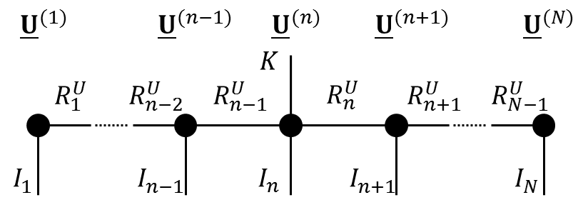
Figure 4: Tensor network diagram for a group of vectors in block-$n$ TT format

In order to clearly state the relationship between the TT-cores of the vectors $\mathbf{u}_{1},\ldots,\mathbf{u}_{K}$ in vector TT format and the matrix $\mathbf{U}$ in block-$n$ TT format, we first define the full-rank condition for block-$n$ TT decompositions, similarly as in [18].

Definition 2.1 (full-rank condition, [18]).

For an arbitrary tensor $\underline{\mathbf{U}}\in\mathbb{R}^{I_{1}\times\cdots\times I_{n-1}\times K\times I_{n}\times\cdots\times I_{N}}$, a block-$n$ TT decomposition

$$\underline{\mathbf{U}}=\underline{\mathbf{U}}^{(1)}\bullet\underline{\mathbf{U}}^{(2)}\bullet\cdots\bullet\underline{\mathbf{U}}^{(N)}$$ (19)

of TT-ranks $R^{U}_{1},\ldots,R^{U}_{N-1}$ is called minimal or fulfilling the full-rank condition if all the TT-cores have full left and right ranks, i.e.,

$$R_{m-1}=rank\left(\mathbf{U}^{(m)}_{(1)}\right),\quad R_{m}=rank\left(\mathbf{U}^{(m)}_{(3)}\right),\quad\text{for }m=1,\ldots,n-1,n+1,\ldots,N,$$ (20)

and

$$R_{n-1}=rank\left(\mathbf{U}^{(n)}_{(1)}\right),\quad R_{n}=rank\left(\mathbf{U}^{(n)}_{(4)}\right).$$ (21)

In principle, any collection of vectors $\mathbf{u}_{1},\ldots,\mathbf{u}_{K}\in\mathbb{R}^{I_{1}I_{2}\cdots I_{N}}$ can be combined and a block-$n$ TT format for $\mathbf{U}=[\mathbf{u}_{1},\ldots,\mathbf{u}_{K}]$ can be computed by the TT-SVD algorithm proposed in [34]. As described in [18], a minimal block-$n$ TT decomposition for $\mathbf{U}$ can be computed by applying SVD without truncation successively. Moreover, the TT-ranks for $\mathbf{U}$ are determined uniquely, which will be called minimal TT-ranks.

Given a block-$n$ TT decomposition (17) of the tensor $\underline{\mathbf{U}}\in\mathbb{R}^{I_{1}\times\cdots\times I_{n-1}\times K\times I_{n}\times\cdots\times I_{N}}$, we define the contracted products of the left or right TT-cores by

$$\underline{\mathbf{U}}^{<m}=\underline{\mathbf{U}}^{(1)}\bullet\cdots\bullet\underline{\mathbf{U}}^{(m-1)}\in\mathbb{R}^{I_{1}\times\cdots\times I_{m-1}\times R_{m-1}}$$ (22)

for $m=1,2,\ldots,n$, and

$$\underline{\mathbf{U}}^{>m}=\underline{\mathbf{U}}^{(m+1)}\bullet\cdots\bullet\underline{\mathbf{U}}^{(N)}\in\mathbb{R}^{R_{m}\times I_{m+1}\times\cdots\times I_{N}}$$ (23)

for $m=n,n+1,\ldots,N$. We define that $\underline{\mathbf{U}}^{<1}=\underline{\mathbf{U}}^{>N}=1$. The tensors $\underline{\mathbf{U}}^{\leq m}$ and $\underline{\mathbf{U}}^{\geq m}$ are defined in the same manner. The mode-$m$ matricization of $\underline{\mathbf{U}}^{<m}$ and the mode-$1$ matricization of $\underline{\mathbf{U}}^{>m}$ are written by

$$\begin{split}\mathbf{U}^{<m}_{(m)}&\in\mathbb{R}^{R_{m-1}\times I_{1}I_{2}\cdots I_{m-1}},\\ \mathbf{U}^{>m}_{(1)}&\in\mathbb{R}^{R_{m}\times I_{m+1}I_{m+2}\cdots I_{N}}.\end{split}$$ (24)

We can easily derive the conditions on the vectors $\mathbf{u}_{1},\ldots,\mathbf{u}_{K}$ based on a minimal block-$n$ TT decomposition (17) of the matrix $\mathbf{U}$ of TT-ranks $R_{1}^{U},\ldots,R_{N-1}^{U}$ as follows.

Proposition 2.2.

Suppose that the matrix $\mathbf{U}=[\mathbf{u}_{1},\ldots,\mathbf{u}_{K}]\in\mathbb{R}^{I_{1}I_{2}\cdots I_{N}\times K}$ has the minimal block-$n$ TT decomposition (17) of TT-ranks $R_{1}^{U},\ldots,R_{N-1}^{U}$. Let

$$\mathbf{U}_{k,m}\in\mathbb{R}^{I_{1}I_{2}\cdots I_{m}\times I_{m+1}\cdots I_{N}}$$ (25)

denote the matrix obtained by reshaping the vector $\mathbf{u}_{k}\in\mathbb{R}^{I_{1}I_{2}\cdots I_{N}}$, i.e, $\mathbf{u}_{k}=\text{vec}(\mathbf{U}_{k,m})$, for $m=1,2,\ldots,N$. Then, we can show that

$$\text{span}\left(\mathbf{U}_{k,m}\right)\subset\text{span}\left(\left(\mathbf{U}^{<m+1}_{(m+1)}\right)^{\mathrm{T}}\right),\quad m=1,2,\ldots,n-1,$$ (26)

and

$$\text{span}\left(\mathbf{U}_{k,m}^{\mathrm{T}}\right)\subset\text{span}\left(\left(\mathbf{U}^{>m}_{(1)}\right)^{\mathrm{T}}\right),\quad m=n,n+1,\ldots,N,$$ (27)

where $\text{span}(\mathbf{A})$ is the column space of a matrix $\mathbf{A}$. Consequently, the minimal TT-ranks, $R^{U}_{k,1},\ldots,R^{U}_{k,N-1}$, of the vector $\mathbf{u}_{k}$ are bounded by the minimal TT-ranks, $R^{U}_{1},\ldots,R^{U}_{N-1}$, of $\mathbf{U}$, i.e.,

$$R^{U}_{k,m}\leq R^{U}_{m},\quad m=1,\ldots,N-1,\ k=1,\ldots,K.$$ (28)

Proof.

Since the vector $\mathbf{u}_{k}$ is represented in vector TT format as in (18), the matrices $\mathbf{U}_{k,m}$ are represented by

$$\begin{split}\mathbf{U}_{k,m}&=\left(\mathbf{U}^{<m+1}_{(m+1)}\right)^{\mathrm{T}}\mathbf{U}^{>m}_{k,(1)},\quad m=1,2,\ldots,n-1,\\ \mathbf{U}_{k,m}&=\left(\mathbf{U}^{<m+1}_{k,(m+1)}\right)^{\mathrm{T}}\mathbf{U}^{>m}_{(1)},\quad m=n,n+1,\ldots,N,\end{split}$$ (29)

where $\mathbf{U}^{>m}_{k,(1)}$ and $\mathbf{U}^{<m+1}_{k,(m+1)}$ are the matricizations of subtensors of $\underline{\mathbf{U}}^{>m}$ and $\underline{\mathbf{U}}^{<m+1}$. It holds that the minimal TT-ranks $R^{U}_{k,m}=rank(\mathbf{U}_{k,m})$ by [18]. This proves the Proposition 2.2. ∎

2.5 Matricization of Block TT Format

A matrix $\mathbf{U}\in\mathbb{R}^{I_{1}I_{2}\cdots I_{N}\times K}$ having a block-$n$ TT decomposition (17) can be expressed as a product of matrices, which is useful for describing algorithms based on block TT formats. For a fixed $n$, frame matrices are defined as follows.

Definition 2.3 (Frame matrix, [8, 19, 25]).

The frame matrices $\mathbf{U}^{\neq n}\in\mathbb{R}^{I_{1}I_{2}\cdots I_{N}\times R_{n-1}I_{n}R_{n}}$ and $\mathbf{U}^{\neq n-1,n}\in\mathbb{R}^{I_{1}I_{2}\cdots I_{N}\times R_{n-2}I_{n-1}I_{n}R_{n}}$ are defined by

$$\mathbf{U}^{\neq n}=\left(\mathbf{U}^{>n}_{(1)}\right)^{\mathrm{T}}\otimes\mathbf{I}_{I_{n}}\otimes\left(\mathbf{U}^{<n}_{(n)}\right)^{\mathrm{T}}$$ (30)

and

$$\mathbf{U}^{\neq n-1,n}=\left(\mathbf{U}^{>n}_{(1)}\right)^{\mathrm{T}}\otimes\mathbf{I}_{I_{n}}\otimes\mathbf{I}_{I_{n-1}}\otimes\left(\mathbf{U}^{<n-1}_{(n-1)}\right)^{\mathrm{T}}.$$ (31)

The block-$n$ TT tensor $\underline{\mathbf{U}}$ is written by $\underline{\mathbf{U}}=\underline{\mathbf{U}}^{<n}\bullet\underline{\mathbf{U}}^{(n)}\bullet\underline{\mathbf{U}}^{>n},$ where the $n$th TT-core is a 4th order tensor, $\underline{\mathbf{U}}^{(n)}\in\mathbb{R}^{R_{n-1}\times K\times I_{n}\times R_{n}}$. The matrix $\mathbf{U}$ is the transpose of the mode-$n$ matricization $\mathbf{U}_{(n)}\in\mathbb{R}^{K\times I_{1}I_{2}\cdots I_{N}}$ of $\underline{\mathbf{U}}$, which can be expressed by

$$\begin{split}\mathbf{U}_{(n)}&=\left(\underline{\mathbf{U}}^{<n}\bullet\underline{\mathbf{U}}^{(n)}\bullet\underline{\mathbf{U}}^{>n}\right)_{(n)}\\ &=\left(\underline{\mathbf{U}}^{(n)}\times_{1}\left(\mathbf{U}^{<n}_{(n)}\right)^{\mathrm{T}}\times_{4}\left(\mathbf{U}^{>n}_{(1)}\right)^{\mathrm{T}}\right)_{(2)}\\ &=\mathbf{U}^{(n)}_{(2)}\left(\mathbf{U}^{>n}_{(1)}\otimes\mathbf{I}_{I_{n}}\otimes\mathbf{U}^{<n}_{(n)}\right).\end{split}$$ (32)

Next, we consider the contraction of two neighboring core tensors as

$$\underline{\mathbf{U}}^{(n-1,n)}=\underline{\mathbf{U}}^{(n-1)}\bullet\underline{\mathbf{U}}^{(n)}\in\mathbb{R}^{R_{n-2}\times I_{n-1}\times K\times I_{n}\times R_{n}}.$$ (33)

Then the block-$n$ TT tensor $\underline{\mathbf{U}}$ is written by $\underline{\mathbf{U}}=\underline{\mathbf{U}}^{<n-1}\bullet\underline{\mathbf{U}}^{(n-1,n)}\bullet\underline{\mathbf{U}}^{>n},$ and we can get an another expression for the mode-$n$ matricization as

$$\mathbf{U}_{(n)}=\mathbf{U}^{(n-1,n)}_{(3)}\left(\mathbf{U}^{>n}_{(1)}\otimes\mathbf{I}_{I_{n}}\otimes\mathbf{I}_{I_{n-1}}\otimes\mathbf{U}^{<n-1}_{(n-1)}\right)\in\mathbb{R}^{K\times I_{1}I_{2}\cdots I_{N}}.$$ (34)

From (32) and (34), the matrix $\mathbf{U}=[\mathbf{u}_{1},\mathbf{u}_{2},\ldots,\mathbf{u}_{K}]\in\mathbb{R}^{I_{1}I_{2}\cdots I_{N}\times K}$ in block-$n$ TT format can be written by

$$\mathbf{U}=\mathbf{U}^{\neq n}\mathbf{U}^{(n)},\qquad n=1,2,\ldots,N,$$ (35)

where $\mathbf{U}^{(n)}=(\mathbf{U}^{(n)}_{(2)})^{\mathrm{T}}\in\mathbb{R}^{R_{n-1}I_{n}R_{n}\times K}$, and by

$$\mathbf{U}=\mathbf{U}^{\neq n-1,n}\mathbf{U}^{(n-1,n)},\qquad n=2,3,\ldots,N,$$ (36)

where $\mathbf{U}^{(n-1,n)}=(\mathbf{U}^{(n-1,n)}_{(3)})^{\mathrm{T}}\in\mathbb{R}^{R_{n-2}I_{n-1}I_{n}R_{n}\times K}$.

2.6 Orthogonalization of Core Tensors

Definition 2.4 (Left- and right-orthogonality, [18]).

A 3rd order core tensor $\underline{\mathbf{U}}^{(m)}\in\mathbb{R}^{R_{m-1}\times I_{m}\times R_{m}}$ is called left-orthogonal if

$$\mathbf{U}_{(3)}^{(m)}\left(\mathbf{U}_{(3)}^{(m)}\right)^{\mathrm{T}}=\mathbf{I}_{R_{m}},$$ (37)

and right-orthogonal if

$$\mathbf{U}_{(1)}^{(m)}\left(\mathbf{U}_{(1)}^{(m)}\right)^{\mathrm{T}}=\mathbf{I}_{R_{m-1}}.$$ (38)

We can show that the matricizations $\mathbf{U}^{<n}_{(n)}$ and $\mathbf{U}^{>n}_{(1)}$ have orthonormal rows if the left core tensors $\underline{\mathbf{U}}^{(1)},\ldots,\underline{\mathbf{U}}^{(n-1)}$ are left-orthogonalized and the right core tensors $\underline{\mathbf{U}}^{(n+1)},\ldots,\underline{\mathbf{U}}^{(N)}$ are right-orthogonalized [29]. Consequently, the frame matrices $\mathbf{U}^{\neq n}$ and $\mathbf{U}^{\neq n-1,n}$ have orthonormal columns if each of the left and right core tensors is properly orthogonalized. From the expressions (35) and (36), we can guarantee orthonormality of the columns of $\mathbf{U}$ by orthogonalizing the TT-cores. Figure 5 shows a tensor network diagram for the matrix $\mathbf{U}$ in block-$n$ TT format where all the core tensors are either left or right orthogonalized except the $n$th core tensor. In this case we can guarantee that the frame matrices $\mathbf{U}^{\neq n}$ and $\mathbf{U}^{\neq n-1,n}$ have orthonormal columns.

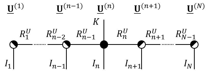
Figure 5: Tensor network diagram for a group of vectors in block-$n$ TT format whose TT-cores are either left- or right-orthogonalized except the $n$th TT-core. The left- or right-orthogonalized tensors are represented by half-filled circles.

3 SVD Algorithms Based on Block TT Format

In this section, we describe the new SVD algorithms, which we call the ALS for SVD (ALS-SVD) and MALS for SVD (MALS-SVD).

In the ALS-SVD and MALS-SVD, the left and right singular vectors $\mathbf{U}=[\mathbf{u}_{1},\ldots,\mathbf{u}_{N}]\in\mathbb{R}^{I_{1}I_{2}\cdots I_{N}\times K}$ and $\mathbf{V}=[\mathbf{v}_{1},\ldots,\mathbf{v}_{N}]\in\mathbb{R}^{J_{1}J_{2}\cdots J_{N}\times K}$ are initialized with block-$N$ TT formats. For each $n\in\{1,2,\ldots,N\}$, we suppose that $\mathbf{U}$ and $\mathbf{V}$ are represented by block-$n$ TT formats

$$\underline{\mathbf{U}}=\underline{\mathbf{U}}^{(1)}\bullet\underline{\mathbf{U}}^{(2)}\bullet\cdots\bullet\underline{\mathbf{U}}^{(N)},\qquad\underline{\mathbf{V}}=\underline{\mathbf{V}}^{(1)}\bullet\underline{\mathbf{V}}^{(2)}\bullet\cdots\bullet\underline{\mathbf{V}}^{(N)},$$ (39)

where the $n$th core tensors $\underline{\mathbf{U}}^{(n)}\in\mathbb{R}^{R^{U}_{n-1}\times K\times I_{n}\times R^{U}_{n}}$ and $\underline{\mathbf{V}}^{(n)}\in\mathbb{R}^{R^{V}_{n-1}\times K\times J_{n}\times R^{V}_{n}}$ are 4th order tensors and the other core tensors are 3rd order tensors. We suppose that all the $1,2,\ldots,(n-1)$th core tensors are left-orthogonalized and all the $n+1,n+2,\ldots,N$th core tensors are right-orthogonalized.

Figure 6 illustrates the tensor network diagrams representing the $\text{trace}\left(\mathbf{U}^{\mathrm{T}}\mathbf{AV}\right)$ in the maximization problem (1). Note that the matrix $\mathbf{A}\in\mathbb{R}^{I_{1}I_{2}\cdots I_{N}\times J_{1}J_{2}\cdots J_{N}}$ is in matrix TT format. In the algorithms we don’t need to compute the large-scale matrix-by-vector products $\mathbf{AV}$ or $\mathbf{A}^{\mathrm{T}}\mathbf{U}$. All the necessary basic computations are performed based on efficient contractions of core tensors.

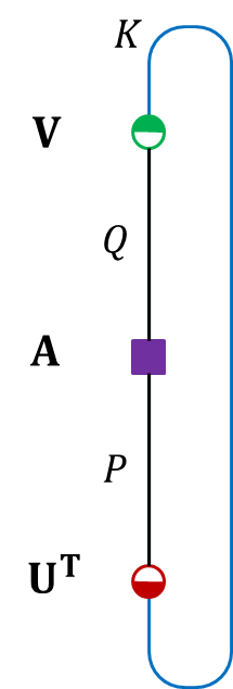
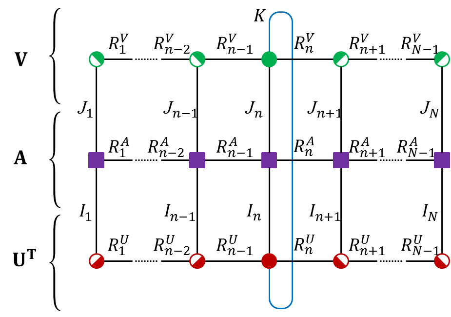
(a)	(b)

Figure 6: Tensor network diagrams for the $\text{trace}\left(\mathbf{U}^{\mathrm{T}}\mathbf{AV}\right)$ in the maximization problem (1). (a) $\mathbf{U}\in\mathbb{R}^{P\times K}$ and $\mathbf{V}\in\mathbb{R}^{Q\times K}$ are matrices with orthonormal column vectors and $\mathbf{A}\in\mathbb{R}^{P\times Q}$ is a matrix. (b) The matrices $\mathbf{U}$ and $\mathbf{V}$ are represented in block-$n$ TT format and the matrix $\mathbf{A}$ is represented in matrix TT format, where $P=I_{1}I_{2}\cdots I_{N}$ and $Q=J_{1}J_{2}\cdots J_{N}$. Each of the TT-cores of $\mathbf{U}$ and $\mathbf{V}$ are orthogonalized in order to keep the orthogonality constraint.

3.1 ALS for SVD Based on Block TT Format

The ALS algorithm for SVD based on block TT format is described in Algorithm 1. Recall that, from (35), the matrices $\mathbf{U}$ and $\mathbf{V}$ of singular vectors are written by

$$\mathbf{U}=\mathbf{U}^{\neq n}\mathbf{U}^{(n)},\qquad\mathbf{V}=\mathbf{V}^{\neq n}\mathbf{V}^{(n)},$$ (40)

where $\mathbf{U}^{(n)}=(\mathbf{U}^{(n)}_{(2)})^{\mathrm{T}}\in\mathbb{R}^{R^{U}_{n-1}I_{n}R^{U}_{n}\times K}$ and $\mathbf{V}^{(n)}=(\mathbf{V}^{(n)}_{(2)})^{\mathrm{T}}\in\mathbb{R}^{R^{V}_{n-1}J_{n}R^{V}_{n}\times K}$. Note that $(\mathbf{U}^{\neq n})^{\mathrm{T}}\mathbf{U}^{\neq n}=\mathbf{I}_{R^{U}_{n-1}I_{n}R^{U}_{n}}$ and $(\mathbf{V}^{\neq n})^{\mathrm{T}}\mathbf{V}^{\neq n}=\mathbf{I}_{R^{V}_{n-1}I_{n}R^{V}_{n}}.$ Given that all the core tensors are fixed except the $n$th core tensors, the maximization problem (1) is reduced to the smaller optimization problem as

$$\begin{split}\mathop{\text{maximize}}_{\mathbf{U}^{(n)},\mathbf{V}^{(n)}}&\qquad\text{trace}\left(\mathbf{U}^{\mathrm{T}}\mathbf{AV}\right)=\text{trace}\left((\mathbf{U}^{(n)})^{\mathrm{T}}\overline{\mathbf{A}}_{n}\mathbf{V}^{(n)}\right)\\ \text{subject to}&\qquad(\mathbf{U}^{(n)})^{\mathrm{T}}\mathbf{U}^{(n)}=(\mathbf{V}^{(n)})^{\mathrm{T}}\mathbf{V}^{(n)}=\mathbf{I}_{K},\end{split}$$ (41)

where the matrix $\overline{\mathbf{A}}_{n}$ is defined by

$$\overline{\mathbf{A}}_{n}=(\mathbf{U}^{\neq n})^{\mathrm{T}}\mathbf{A}\mathbf{V}^{\neq n}\in\mathbb{R}^{R^{U}_{n-1}I_{n}R^{U}_{n}\times R^{V}_{n-1}J_{n}R^{V}_{n}}.$$ (42)

We call $\overline{\mathbf{A}}_{n}$ as the projected matrix. In the case that the TT-ranks $\{R^{U}_{n}\}$ and $\{R^{V}_{n}\}$ are small enough, the projected matrix $\overline{\mathbf{A}}_{n}$ has much smaller sizes than $\mathbf{A}\in\mathbb{R}^{I_{1}I_{2}\cdots I_{N}\times J_{1}J_{2}\cdots J_{N}}$, so that any standard and efficient SVD algorithms can be applied. In Section 3.3, we will describe how the reduced local optimization problem (41) can be efficiently solved. In practice, the matrix $\overline{\mathbf{A}}_{n}$ don’t need to be computed explicitly. Instead, the local matrix-by-vector multiplications $\overline{\mathbf{A}}_{n}^{\mathrm{T}}\mathbf{u}$ and $\overline{\mathbf{A}}_{n}\mathbf{v}$ for any vectors $\mathbf{u}\in\mathbb{R}^{R^{U}_{n-1}I_{n}R^{U}_{n}}$ and $\mathbf{v}\in\mathbb{R}^{R^{V}_{n-1}J_{n}R^{V}_{n}}$ are computed more efficiently based on the contractions of core tensors of $\mathbf{U}$, $\mathbf{A}$, and $\mathbf{V}$.

1

Input : $\mathbf{A}\in\mathbb{R}^{I_{1}I_{2}\cdots I_{N}\times J_{1}J_{2}\cdots J_{N}}$ in matrix TT format, $K\geq 2$, $\delta\geq 0$ (truncation parameter)

Output : Dominant singular values $\mathbf{\Sigma}=\text{diag}(\sigma_{1},\sigma_{2},\ldots,\sigma_{K})$ and corresponding singular vectors $\mathbf{U}\in\mathbb{R}^{I_{1}I_{2}\cdots I_{N}\times K}$ and $\mathbf{V}\in\mathbb{R}^{J_{1}J_{2}\cdots J_{N}\times K}$ in block-$N$ TT format with TT-ranks $R^{U}_{1},R^{U}_{2},\ldots,R^{U}_{N-1}$ for $\mathbf{U}$ and $R^{V}_{1},R^{V}_{2},\ldots,R^{V}_{N-1}$ for $\mathbf{V}$.

2 Initialize $\mathbf{U}$ and $\mathbf{V}$ in block-$N$ TT format with left-orthogonalized TT-cores $\underline{\mathbf{U}}^{(1)},\ldots,\underline{\mathbf{U}}^{(N-1)},\underline{\mathbf{V}}^{(1)},\ldots,\underline{\mathbf{V}}^{(N-1)}$ and small TT-ranks $R_{1}^{U},\ldots,R_{N-1}^{U},R_{1}^{V},\ldots,R_{N-1}^{V}$.

3 Compute the 3rd order tensors $\underline{\mathbf{L}}^{<1},\ldots,\underline{\mathbf{L}}^{<N}$ recursively by (59) and (60). Set $\underline{\mathbf{R}}^{>N}=1$.

4 repeat

5       for $n=N,N-1,\ldots,2$ do right-to-left half sweep

             // Optimization

6             Compute $\mathbf{U}^{(n)}$ and $\mathbf{V}^{(n)}$ by solving (41).

7             Update the singular values $\mathbf{\Sigma}=(\mathbf{U}^{(n)})^{\mathrm{T}}\overline{\mathbf{A}}_{n}\mathbf{V}^{(n)}$.

             // Matrix Factorization and Adaptive Rank Estimation

8             Reshape $\underline{\mathbf{U}}^{(n)}=reshape(\mathbf{U}^{(n)},[R^{U}_{n-1},I_{n},R^{U}_{n},K])$, $\underline{\mathbf{V}}^{(n)}=reshape(\mathbf{V}^{(n)},[R^{V}_{n-1},J_{n},R^{V}_{n},K]).$

9             Compute $\delta$-truncated SVD:

$$\begin{split}[\mathbf{U}_{1},\mathbf{S}_{1},\mathbf{V}_{1}]&=\mathrm{SVD}_{\delta}\left(\mathbf{U}^{(n)}_{(\{1,4\}\times\{2,3\})}\right),\\ [\mathbf{U}_{2},\mathbf{S}_{2},\mathbf{V}_{2}]&=\mathrm{SVD}_{\delta}\left(\mathbf{V}^{(n)}_{(\{1,4\}\times\{2,3\})}\right).\end{split}$$ (43)

10             Set $R^{U,new}=rank(\mathbf{V}_{1})$, $R^{V,new}=rank(\mathbf{V}_{2})$.

11             Update TT-cores

$$\begin{split}\underline{\mathbf{U}}^{(n)}&=reshape(\mathbf{V}_{1}^{\text{T}},[R^{U,new},I_{n},R^{U}_{n}]),\\ \underline{\mathbf{V}}^{(n)}&=reshape(\mathbf{V}_{2}^{\text{T}},[R^{V,new},J_{n},R^{V}_{n}]).\end{split}$$ (44)

12             Compute multiplications

$$\begin{split}\mathbf{U}^{(n-1)}&=reshape(\underline{\mathbf{U}}^{(n-1)},[R^{U}_{n-2}I_{n-1},R^{U}_{n-1}])\cdot reshape(\mathbf{U}_{1}\mathbf{S}_{1},[R^{U}_{n-1},KR^{U,new}]),\\ \mathbf{V}^{(n-1)}&=reshape(\underline{\mathbf{V}}^{(n-1)},[R^{V}_{n-2}J_{n-1},R^{V}_{n-1}])\cdot reshape(\mathbf{V}_{1}\mathbf{S}_{1},[R^{V}_{n-1},KR^{V,new}]).\end{split}$$ (45)

13             Update TT-cores

$$\begin{split}\underline{\mathbf{U}}^{(n-1)}&=reshape(\mathbf{U}^{(n-1)},[R^{U}_{n-2},I_{n-1},K,R^{U,new}]),\\ \underline{\mathbf{V}}^{(n-1)}&=reshape(\mathbf{V}^{(n-1)},[R^{V}_{n-2},J_{n-1},K,R^{V,new}]).\end{split}$$ (46)

14             Update TT-ranks $R^{U}_{n-1}=R^{U,new}$, $R^{V}_{n-1}=R^{V,new}$.

15             Compute the 3rd order tensor $\underline{\mathbf{R}}^{>n-1}$ by (62)

16       end for

17      for $n=1,2,\ldots,N-1$ do

18             Carry out left-to-right half sweep similarly

19       end for

20      

21until a stopping criterion is met (See Section 3.5.2);

Algorithm 1 ALS for SVD based on block TT format

We note that the $K$ dominant singular values $\mathbf{\Sigma}=\text{diag}(\sigma_{1},\sigma_{2},\ldots,\sigma_{K})$ are equivalent to the $K$ dominant singular values of the projected matrix $\overline{\mathbf{A}}_{n}$ in the sense that $\mathbf{\Sigma}=\mathbf{U}^{\mathrm{T}}\mathbf{AV}=(\mathbf{U}^{(n)})^{\mathrm{T}}\overline{\mathbf{A}}_{n}\mathbf{V}^{(n)}$. Hence, the singular values are updated at each iteration by the singular values estimated by the standard SVD algorithms for the reduced optimization problem (41).

The TT-ranks of block TT formats are adaptively determined by separating the mode corresponding to the size $K$ from the $n$th TT-cores by using $\delta$-truncated SVD. We say that the iteration is during the right-to-left half sweep if the mode of the size $K$ is moving from the $n$th TT-core to the $(n-1)$th TT-core, whereas the iteration is during the left-to-right halft sweep if the mode of the size $K$ moves from the $n$th TT core to the $(n+1)$th TT-core. During the right-to-left half sweep, the $\delta$-truncated SVD decomposes unfolded $n$th TT-cores as

$$\begin{split}\mathbf{U}^{(n)}_{(\{1,4\}\times\{2,3\})}&=\mathbf{U}_{1}\mathbf{S}_{1}\mathbf{V}_{1}^{\mathrm{T}}+\mathbf{E}_{1}\in\mathbb{R}^{R^{U}_{n-1}K\times I_{n}R^{U}_{n}},\\ \mathbf{V}^{(n)}_{(\{1,4\}\times\{2,3\})}&=\mathbf{U}_{2}\mathbf{S}_{2}\mathbf{V}_{2}^{\mathrm{T}}+\mathbf{E}_{2}\in\mathbb{R}^{R^{V}_{n-1}K\times J_{n}R^{V}_{n}},\end{split}$$ (47)

where $\|\mathbf{E}_{1}\|_{\mathrm{F}}\leq\delta\|\underline{\mathbf{U}}^{(n)}\|_{\mathrm{F}}$ and $\|\mathbf{E}_{2}\|_{\mathrm{F}}\leq\delta\|\underline{\mathbf{V}}^{(n)}\|_{\mathrm{F}}$. Then, the TT-ranks are updated by $R^{U}_{n-1}=rank(\mathbf{V}_{1})$ and $R^{V}_{n-1}=rank(\mathbf{V}_{2})$, which are simply the numbers of columns of $\mathbf{V}_{1}$ and $\mathbf{V}_{2}$. The $n$th TT-cores are updated by reshaping $\mathbf{V}_{1}^{\mathrm{T}}$ and $\mathbf{V}_{2}^{\mathrm{T}}$. Note that in the case that $K=1$, the TT-ranks $R^{U}_{n-1}$ and $R^{V}_{n-1}$ cannot be increased because, for example,

$$R^{U,new}=rank(\mathbf{V}_{1})=rank(\mathbf{U}_{1}\mathbf{S}_{1})\leq R^{U}_{n-1}K=R^{U}_{n-1}.$$ (48)

Figure 7 illustrates the ALS scheme based on block TT format for the first two iterations. In the figure, the $n$th TT-core is computed by a local optimization algorithm for the maximization problem (41), and then the block-$n$ TT format is converted to the block-$(n-1)$ TT format via the $\delta$-truncated SVD.

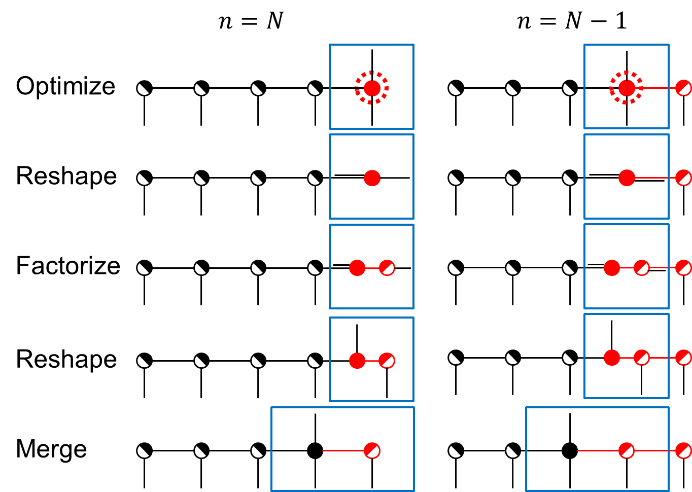
Figure 7: Illustration of the ALS scheme based on block TT format for the first two iterations during right-to-left half sweep

3.2 MALS for SVD Based on Block TT Format

In the ALS scheme, the TT-ranks cannot be adaptively determined if $K=1$. Moreover, a small value of $K$ often slows the rate of convergence because of the relatively slow growth of TT-ranks, which is described in the inequality in (48). On the other hand, the MALS scheme shows relatively fast convergence and the TT-ranks can be adaptively determined even if $K=1$.

The MALS algorithm for SVD is described in Algorithm 2. In the MALS scheme, the right-to-left half sweep means the iterations when the $(n-1)$th and $n$th TT-cores are updated for $n=N,N-1,\ldots,2$, and the left-to-right half sweep means the iterations when the $n$th and $(n+1)$th TT-cores are updated for $n=1,2,\ldots,N-1$. At each iteration during the right-to-left half sweep, the left and right singular vectors $\mathbf{U}$ and $\mathbf{V}$ are represented in block-$n$ TT format. From (36), the matrices $\mathbf{U}$ and $\mathbf{V}$ are written by

$$\mathbf{U}=\mathbf{U}^{\neq n-1,n}\mathbf{U}^{(n-1,n)},\qquad\mathbf{V}=\mathbf{V}^{\neq n-1,n}\mathbf{V}^{(n-1,n)}$$ (49)

for $n=2,3,\ldots,N,$ where $\mathbf{U}^{(n-1,n)}\in\mathbb{R}^{R^{U}_{n-2}I_{n-1}I_{n}R^{U}_{n}\times K}$ and $\mathbf{V}^{(n-1,n)}\in\mathbb{R}^{R^{V}_{n-2}J_{n-1}J_{n}R^{V}_{n}\times K}$ are matricizations of the merged TT-cores $\underline{\mathbf{U}}^{(n-1)}\bullet\underline{\mathbf{U}}^{(n)}$ and $\underline{\mathbf{V}}^{(n-1)}\bullet\underline{\mathbf{V}}^{(n)}$. Given that all the TT-cores are fixed except the $(n-1)$th and $n$th TT-cores, the large-scale optimization problem (1) is reduced to

$$\begin{split}\mathop{\text{maximize}}_{\mathbf{U}^{(n-1,n)},\mathbf{V}^{(n-1,n)}}&\qquad\text{trace}\left(\mathbf{U}^{\mathrm{T}}\mathbf{AV}\right)=\text{trace}\left((\mathbf{U}^{(n-1,n)})^{\mathrm{T}}\overline{\mathbf{A}}_{n-1,n}\mathbf{V}^{(n-1,n)}\right)\\ \text{subject to}&\qquad(\mathbf{U}^{(n-1,n)})^{\mathrm{T}}\mathbf{U}^{(n-1,n)}=(\mathbf{V}^{(n-1,n)})^{\mathrm{T}}\mathbf{V}^{(n-1,n)}=\mathbf{I}_{K},\end{split}$$ (50)

where

$$\overline{\mathbf{A}}_{n-1,n}=(\mathbf{U}^{\neq n-1,n})^{\mathrm{T}}\mathbf{A}\mathbf{V}^{\neq n-1,n}\in\mathbb{R}^{R^{U}_{n-2}I_{n-1}I_{n}R^{U}_{n}\times R^{V}_{n-2}J_{n-1}J_{n}R^{V}_{n}}$$ (51)

is called as the projected matrix.

Figure 8 illustrates the MALS scheme. In the MALS, two neighboring core tensors are first merged and updated by solving the optimization problem (50). Then, the $\delta$-truncated SVD factorizes it back into two core tensors. The block-$n$ TT format is transformed into either the block-$(n-1)$ TT format or the block-$(n+1)$ TT format consequently.

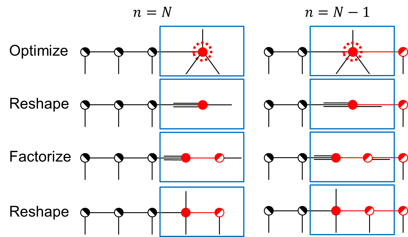
Figure 8: Illustration of the MALS scheme based on block TT format for the first two iterations during right-to-left half sweep

1

Input : $\mathbf{A}\in\mathbb{R}^{I_{1}I_{2}\cdots I_{N}\times J_{1}J_{2}\cdots J_{N}}$ in matrix TT format, $K\geq 1$, $\delta\geq 0$ (truncation parameter)

Output : Dominant singular values $\mathbf{\Sigma}=\text{diag}(\sigma_{1},\sigma_{2},\ldots,\sigma_{K})$ and corresponding singular vectors $\mathbf{U}\in\mathbb{R}^{I_{1}I_{2}\cdots I_{N}\times K}$ and $\mathbf{V}\in\mathbb{R}^{J_{1}J_{2}\cdots J_{N}\times K}$ in block-$N$ TT format with TT-ranks $R^{U}_{1},R^{U}_{2},\ldots,R^{U}_{N-1}$ for $\mathbf{U}$ and $R^{V}_{1},R^{V}_{2},\ldots,R^{V}_{N-1}$ for $\mathbf{V}$.

2 Initialize $\mathbf{U}$ and $\mathbf{V}$ in block-$N$ TT format with left-orthogonalized TT-cores $\underline{\mathbf{U}}^{(1)},\ldots,\underline{\mathbf{U}}^{(N-2)},\underline{\mathbf{V}}^{(1)},\ldots,\underline{\mathbf{V}}^{(N-2)}$ and small TT-ranks $R_{1}^{U},\ldots,R_{N-1}^{U},R_{1}^{V},\ldots,R_{N-1}^{V}$.

3 Compute the 3rd order tensors $\underline{\mathbf{L}}^{<1},\ldots,\underline{\mathbf{L}}^{<N-1}$ recursively by (59) and (60). Set $\underline{\mathbf{R}}^{>N}=1$.

4 repeat

5       for $n=N,N-1,\ldots,2$ do right-to-left half sweep

             // Optimization

6             Compute $\mathbf{U}^{(n-1,n)}$ and $\mathbf{V}^{(n-1,n)}$ by solving (50).

7             Update the singular values $\mathbf{\Sigma}=(\mathbf{U}^{(n-1,n)})^{\mathrm{T}}\overline{\mathbf{A}}_{n-1,n}\mathbf{V}^{(n-1,n)}$.

             // Matrix Factorization and Adaptive Rank Estimation

8             Reshape $\underline{\mathbf{U}}^{(n-1,n)}=reshape(\mathbf{U}^{(n-1,n)},[R^{U}_{n-2},I_{n-1},I_{n},R^{U}_{n},K])$, $\underline{\mathbf{V}}^{(n-1,n)}=reshape(\mathbf{V}^{(n-1,n)},[R^{V}_{n-2},J_{n-1},J_{n},R^{V}_{n},K])$.

9             Compute $\delta$-truncated SVD:

$$\begin{split}[\mathbf{U}_{1},\mathbf{S}_{1},\mathbf{V}_{1}]&=\mathrm{SVD}_{\delta}\left(\mathbf{U}^{(n-1,n)}_{(\{1,2,5\}\times\{3,4\})}\right),\\ [\mathbf{U}_{2},\mathbf{S}_{2},\mathbf{V}_{2}]&=\mathrm{SVD}_{\delta}\left(\mathbf{V}^{(n-1,n)}_{(\{1,2,5\}\times\{3,4\})}\right).\end{split}$$ (52)

10             Update TT-ranks $R^{U}_{n-1}=rank(\mathbf{V}_{1})$, $R^{V}_{n-1}=rank(\mathbf{V}_{2})$.

11             Update TT-cores

$$\begin{split}\underline{\mathbf{U}}^{(n)}&=reshape(\mathbf{V}_{1}^{\text{T}},[R^{U}_{n-1},I_{n},R^{U}_{n}]),\\ \underline{\mathbf{V}}^{(n)}&=reshape(\mathbf{V}_{2}^{\text{T}},[R^{V}_{n-1},J_{n},R^{V}_{n}]).\end{split}$$ (53)

12             Update TT-cores

$$\begin{split}\underline{\mathbf{U}}^{(n-1)}&=reshape(\mathbf{U}_{1}\mathbf{S}_{1},[R_{n-2}^{U},I_{n-1},K,R_{n-1}^{U}]),\\ \underline{\mathbf{V}}^{(n-1)}&=reshape(\mathbf{U}_{2}\mathbf{S}_{2},[R_{n-2}^{V},J_{n-1},K,R_{n-1}^{V}]).\end{split}$$ (54)

13             Compute the 3rd order tensor $\underline{\mathbf{R}}^{>n-1}$ by (62)

14       end for

15      for $n=1,2,\ldots,N-1$ do

16             Carry out left-to-right half sweep similarly

17       end for

18      

19until a stopping criterion is met (See Section 3.5.2);

Algorithm 2 MALS for SVD based on block TT format

3.3 Efficient Computation of Projected Matrix-by-Vector Product

In order to solve the reduced optimization problems (41) and (50), we consider the eigenvalue decomposition of the block matrices

$$\overline{\mathbf{B}}_{n}=\begin{bmatrix}\mathbf{0}&\overline{\mathbf{A}}_{n}\\ \overline{\mathbf{A}}_{n}^{\mathrm{T}}&\mathbf{0}\end{bmatrix},\qquad\overline{\mathbf{B}}_{n-1,n}=\begin{bmatrix}\mathbf{0}&\overline{\mathbf{A}}_{n-1,n}\\ \overline{\mathbf{A}}_{n-1,n}^{\mathrm{T}}&\mathbf{0}\end{bmatrix}.$$ (55)

It can be shown that the $K$ largest eigenvalues of $\overline{\mathbf{B}}_{n}$ correspond to the $K$ dominant singular values of the projected matrix $\overline{\mathbf{A}}_{n}$, and the eigenvectors of $\overline{\mathbf{B}}_{n}$ correspond to a concatenation of the left and right singular vectors of $\overline{\mathbf{A}}_{n}$. See Appendix A for more detail. The same holds for $\overline{\mathbf{B}}_{n-1,n}$ and $\overline{\mathbf{A}}_{n-1,n}$.

For computing the eigenvalue decomposition of the above matrices, we don’t need to compute the matrices explicitly, but we only need to compute matrix-by-vector products. Let

$$\mathbf{x}\in\mathbb{R}^{R^{U}_{n-1}I_{n}R^{U}_{n}},\quad\mathbf{y}\in\mathbb{R}^{R^{V}_{n-1}J_{n}R^{V}_{n}},\quad\tilde{\mathbf{x}}\in\mathbb{R}^{R^{U}_{n-2}I_{n-1}I_{n}R^{U}_{n}},\quad\tilde{\mathbf{y}}\in\mathbb{R}^{R^{V}_{n-2}J_{n-1}J_{n}R^{V}_{n}}$$ (56)

be given vectors. Then, the matrix-by-vector products are expressed by

$$\overline{\mathbf{B}}_{n}\begin{bmatrix}\mathbf{x}\\ \mathbf{y}\end{bmatrix}=\begin{bmatrix}\overline{\mathbf{A}}_{n}\mathbf{y}\\ \overline{\mathbf{A}}_{n}^{\mathrm{T}}\mathbf{x}\end{bmatrix},\qquad\overline{\mathbf{B}}_{n-1,n}\begin{bmatrix}\tilde{\mathbf{x}}\\ \tilde{\mathbf{y}}\end{bmatrix}=\begin{bmatrix}\overline{\mathbf{A}}_{n-1,n}\tilde{\mathbf{y}}\\ \overline{\mathbf{A}}_{n-1,n}^{\mathrm{T}}\tilde{\mathbf{x}}\end{bmatrix},$$ (57)

which consist of the projected matrix-by-vector products, $\overline{\mathbf{A}}_{n}\mathbf{y},\overline{\mathbf{A}}_{n}^{\mathrm{T}}\mathbf{x},\overline{\mathbf{A}}_{n-1,n}\tilde{\mathbf{y}},$ and $\overline{\mathbf{A}}_{n-1,n}^{\mathrm{T}}\tilde{\mathbf{x}}$.

The computation of the projected matrix-by-vector products is performed in an iterative way as follows. Let $\mathbf{U}^{(m)}_{i_{m}}=\underline{\mathbf{U}}^{(m)}(:,i_{m},:)$, $\mathbf{A}^{(m)}_{i_{m},j_{m}}=\underline{\mathbf{A}}^{(m)}(:,i_{m},j_{m},:)$, and $\mathbf{V}^{(m)}_{j_{m}}=\underline{\mathbf{V}}^{(m)}(:,j_{m},:)$ be the slice matrices of the three $m$th core tensors for $m\neq n$. Let

$$\mathbf{Z}^{(m)}=\sum_{i_{m}=1}^{I_{m}}\sum_{j_{m}=1}^{J_{m}}\mathbf{U}^{(m)}_{i_{m}}\otimes\mathbf{A}^{(m)}_{i_{m},j_{m}}\otimes\mathbf{V}^{(m)}_{j_{m}}\in\mathbb{R}^{R^{U}_{m-1}R^{A}_{m-1}R^{V}_{m-1}\times R^{U}_{m}R^{A}_{m}R^{V}_{m}}.$$ (58)

We define 3rd order tensors $\underline{\mathbf{L}}^{<m}\in\mathbb{R}^{R^{U}_{m-1}\times R^{A}_{m-1}\times R^{V}_{m-1}}$, $m=1,2,\ldots,n,$ and $\underline{\mathbf{R}}^{>m}\in\mathbb{R}^{R^{U}_{m}\times R^{A}_{m}\times R^{V}_{m}}$, $m=n,n+1,\ldots,N,$ recursively by

$$\text{vec}\left(\underline{\mathbf{L}}^{<1}\right)=1,$$ (59)

$$\text{vec}\left(\underline{\mathbf{L}}^{<m}\right)^{\mathrm{T}}=\text{vec}\left(\underline{\mathbf{L}}^{<m-1}\right)^{\mathrm{T}}\mathbf{Z}^{(m-1)}\in\mathbb{R}^{1\times R^{U}_{m-1}R^{A}_{m-1}R^{V}_{m-1}},\qquad m=2,3,\ldots,n,$$ (60)

and

$$\text{vec}\left(\underline{\mathbf{R}}^{>N}\right)=1,$$ (61)

$$\text{vec}\left(\underline{\mathbf{R}}^{>m}\right)=\mathbf{Z}^{(m+1)}\text{vec}\left(\underline{\mathbf{R}}^{>m+1}\right)\in\mathbb{R}^{R^{U}_{m}R^{A}_{m}R^{V}_{m}\times 1},\qquad m=n,n+1,\ldots,N-1.$$ (62)

Recall that $(\mathbf{U}^{(n)})^{\mathrm{T}}\overline{\mathbf{A}}_{n}\mathbf{V}^{(n)}=\mathbf{U}^{\mathrm{T}}\mathbf{AV}$. Let $\mathbf{u}^{(n)}_{k_{1}}$ and $\mathbf{v}^{(n)}_{k_{2}}$ denote the $k_{1}$th and $k_{2}$th column vectors of the matrices $\mathbf{U}^{(n)}$ and $\mathbf{V}^{(n)}$. From the matrix product representations of the matrix TT and block TT formats (16) and (18), we can show that the $(k_{1},k_{2})$ entry of $(\mathbf{U}^{(n)})^{\mathrm{T}}\overline{\mathbf{A}}_{n}\mathbf{V}^{(n)}$ is expressed by

$$\begin{split}(\mathbf{u}^{(n)}_{k_{1}})^{\mathrm{T}}\overline{\mathbf{A}}_{n}\mathbf{v}^{(n)}_{k_{2}}&=\mathbf{u}_{k_{1}}^{\mathrm{T}}\mathbf{Av}_{k_{2}}\\ &=\mathbf{Z}^{(1)}\cdots\mathbf{Z}^{(n-1)}\left(\sum_{i_{n}=1}^{I_{n}}\sum_{j_{n}=1}^{J_{n}}\mathbf{U}^{(n)}_{k_{1},i_{n}}\otimes\mathbf{A}^{(n)}_{i_{n},j_{n}}\otimes\mathbf{V}^{(n)}_{k_{2},j_{n}}\right)\mathbf{Z}^{(n+1)}\cdots\mathbf{Z}^{(N)}\\ &=\text{vec}\left(\underline{\mathbf{L}}^{<n}\right)^{\mathrm{T}}\left(\sum_{i_{n}=1}^{I_{n}}\sum_{j_{n}=1}^{J_{n}}\mathbf{U}^{(n)}_{k_{1},i_{n}}\otimes\mathbf{A}^{(n)}_{i_{n},j_{n}}\otimes\mathbf{V}^{(n)}_{k_{2},j_{n}}\right)\text{vec}\left(\underline{\mathbf{R}}^{>n}\right),\end{split}$$ (63)

which is the contraction of the tensors $\underline{\mathbf{L}}^{<n},\underline{\mathbf{U}}^{(n)},\underline{\mathbf{A}}^{(n)},\underline{\mathbf{V}}^{(n)},$ and $\underline{\mathbf{R}}^{>n}$. Thus, the computation of $\overline{\mathbf{A}}_{n}\mathbf{y}$ is performed by the contraction of the tensors $\underline{\mathbf{L}}^{<n}$, $\underline{\mathbf{Y}}$, $\underline{\mathbf{A}}^{(n)}$, and $\underline{\mathbf{R}}^{>n}$, where $\underline{\mathbf{Y}}\in\mathbb{R}^{R^{V}_{n-1}\times J_{n}\times R^{V}_{n}}$ is the tensorization of the vector $\mathbf{y}$. In the same way, the computation of $\overline{\mathbf{A}}_{n}^{\mathrm{T}}\mathbf{x}$ is performed by the contraction of the tensors $\underline{\mathbf{L}}^{<n}$, $\underline{\mathbf{X}}$, $\underline{\mathbf{A}}^{(n)}$, and $\underline{\mathbf{R}}^{>n}$, where $\underline{\mathbf{X}}\in\mathbb{R}^{R^{U}_{n-1}\times I_{n}\times R^{U}_{n}}$ is the tensorization of the vector $\mathbf{x}$.

Similarly, we can derive an expression for the projected matrix $\overline{\mathbf{A}}_{n-1,n}$ as

$$\begin{split}&(\mathbf{u}^{(n-1,n)}_{k_{1}})^{\mathrm{T}}\overline{\mathbf{A}}_{n-1,n}\mathbf{v}^{(n-1,n)}_{k_{2}}\\ &=\text{vec}\left(\underline{\mathbf{L}}^{<n-1}\right)^{\mathrm{T}}\left(\sum_{i_{n-1}}\sum_{i_{n}}\sum_{j_{n-1}}\sum_{j_{n}}\mathbf{U}^{(n-1,n)}_{i_{n-1},k_{1},i_{n}}\otimes\left(\mathbf{A}^{(n-1)}_{i_{n-1},j_{n-1}}\mathbf{A}^{(n)}_{i_{n},j_{n}}\right)\otimes\mathbf{V}^{(n-1,n)}_{j_{n-1},k_{2},j_{n}}\right)\text{vec}\left(\underline{\mathbf{R}}^{>n}\right),\end{split}$$ (64)

which is the contraction of the tensors $\underline{\mathbf{L}}^{<n-1}$, $\underline{\mathbf{U}}^{(n-1,n)}$, $\underline{\mathbf{A}}^{(n-1)}$, $\underline{\mathbf{A}}^{(n)}$, $\underline{\mathbf{V}}^{(n-1,n)}$, and $\underline{\mathbf{R}}^{>n}$. Thus, the computation of $\overline{\mathbf{A}}_{n-1,n}\tilde{\mathbf{y}}$ is performed by the contraction of the tensors $\underline{\mathbf{L}}^{<n-1}$, $\widetilde{\underline{\mathbf{Y}}}$, $\underline{\mathbf{A}}^{(n-1)}$, $\underline{\mathbf{A}}^{(n)}$, and $\underline{\mathbf{R}}^{>n}$, where $\widetilde{\underline{\mathbf{Y}}}\in\mathbb{R}^{R^{V}_{n-2}\times J_{n-1}\times J_{n}\times R^{V}_{n}}$ is the tensorization of the vector $\tilde{\mathbf{y}}$. In the same way, the computation of $\overline{\mathbf{A}}_{n}^{\mathrm{T}}\tilde{\mathbf{x}}$ is performed by the contraction of the tensors $\underline{\mathbf{L}}^{<n-1}$, $\widetilde{\underline{\mathbf{X}}}$, $\underline{\mathbf{A}}^{(n-1)}$, $\underline{\mathbf{A}}^{(n)}$, and $\underline{\mathbf{R}}^{>n}$, where $\widetilde{\underline{\mathbf{X}}}\in\mathbb{R}^{R^{U}_{n-2}\times I_{n-1}\times I_{n}\times R^{U}_{n}}$ is the tensorization of the vector $\tilde{\mathbf{x}}$.

Figure 9 illustrates the tensor network diagrams for the computation of the projected matrix-by-vector products $\overline{\mathbf{A}}_{n}\mathbf{y}$ and $\overline{\mathbf{A}}_{n-1,n}\tilde{\mathbf{y}}$ for the vectors $\mathbf{y}\in\mathbb{R}^{R^{V}_{n-1}J_{n}R^{V}_{n}}$ and $\tilde{\mathbf{y}}\in\mathbb{R}^{R^{V}_{n-2}J_{n-1}J_{n}R^{V}_{n}}$. Based on the tensor network diagrams, we can easily specify the sizes of the tensors and how the tensors are contracted with each other.

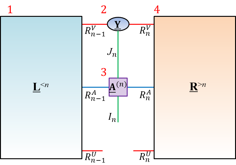
(a) $\overline{\mathbf{A}}_{n}\mathbf{y}$ for ALS-SVD

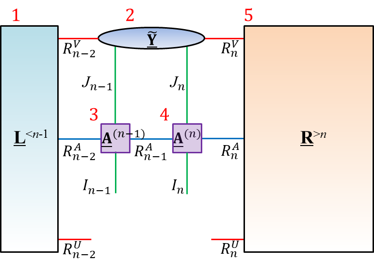
(b) $\overline{\mathbf{A}}_{n-1,n}\tilde{\mathbf{y}}$ for MALS-SVD

Figure 9: Computation of the projected matrix-by-vector products (a) $\overline{\mathbf{A}}_{n}\mathbf{y}$ and (b) $\overline{\mathbf{A}}_{n-1,n}\tilde{\mathbf{y}}$ for solving the reduced optimization problems in the ALS-SVD and MALS-SVD algorithms. (a) The computation of $\overline{\mathbf{A}}_{n}\mathbf{y}$ is carried out by the contraction of $\underline{\mathbf{L}}^{<n}$, $\underline{\mathbf{Y}}$, $\underline{\mathbf{A}}^{(n)}$, and $\underline{\mathbf{R}}^{>n}$. (b) The computation of $\overline{\mathbf{A}}_{n-1,n}\tilde{\mathbf{y}}$ is carried out by the contraction of $\underline{\mathbf{L}}^{<n-1}$, $\widetilde{\underline{\mathbf{Y}}}$, $\underline{\mathbf{A}}^{(n-1)}$, $\underline{\mathbf{A}}^{(n)}$, and $\underline{\mathbf{R}}^{>n}$. An efficient order of contraction is expressed by the numbers on each tensor.

3.4 Computational Complexity

Let $R=max(\{R^{U}_{n}\},\{R^{V}_{n}\})$, $R_{A}=max(\{R^{A}_{n}\})$, and $I=max(\{I_{n}\},\{J_{n}\})$. The computational complexities for the ALS-SVD and MALS-SVD algorithms are summarized in Table 1. We may assume that $K\geq I$ because we usually choose very small values for $I_{n}$ and $J_{n}$, e.g., $I=I_{n}=J_{n}=2$. The computational complexities in Table 1 correspond to each iteration, so the total computational costs for one full sweep (right-to-left and left-to-right half sweeps) grow linearly with the order $N$ given that $R,R_{A},I,$ and $K$ are bounded.

Table 1: Computational complexities of the ALS-SVD and MALS-SVD algorithms for one iteration

	ALS-SVD	MALS-SVD
Orthonormalization	line 5: $\mathcal{O}(K^{2}IR^{2})$	line 5: $\mathcal{O}(K^{2}I^{2}R^{2})$
Projected Matrix-by-	line 5: $\mathcal{O}(KIR_{A}(R+IR_{A})R^{2})$	line 5: $\mathcal{O}(KI^{2}R_{A}(R+IR_{A})R^{2})$
Vector Products
Factorization	line 8: $\mathcal{O}(KI^{2}R^{3})$	line 8: $\mathcal{O}(KI^{3}R^{3})$
Updating Tensor	line 12: $\mathcal{O}(IR_{A}(R+IR_{A})R^{2})$	line 14: $\mathcal{O}(IR_{A}(R+IR_{A})R^{2})$
$\underline{\mathbf{L}}^{<n}$ or $\underline{\mathbf{R}}^{>n}$

At the optimization step at line 5 of the ALS-SVD, standard SVD algorithms perform two important computations [31]: the orthonormalization of a matrix $\mathbf{V}^{(n)}\in\mathbb{R}^{R^{V}_{n-1}J_{n}R^{V}_{n}\times K}$ via QR decomposition, and the projected matrix-by-vector products, $\overline{\mathbf{A}}_{n}\mathbf{V}^{(n)}$. The computational complexity for the QR decomposition is $\mathcal{O}(K^{2}IR^{2})$. For the MALS-SVD, the size of $\mathbf{V}^{(n-1,n)}$ is $R^{V}_{n-2}J_{n-1}J_{n}R^{V}_{n}\times K$, which leads to the computational complexity $\mathcal{O}(K^{2}I^{2}R^{2})$.

The computational complexities for the projected matrix-by-vector products can be conveniently analyzed by using the tensor network diagrams in Figure 9. In Figure 9(a), an efficient order of contraction for computing $\overline{\mathbf{A}}_{n}\mathbf{y}$ is $(\underline{\mathbf{L}}^{<n},\underline{\mathbf{Y}},\underline{\mathbf{A}}^{(n)},\underline{\mathbf{R}}^{>n})$, and its computational complexity is $\mathcal{O}(IR_{A}(R+IR_{A})R^{2})$. Since the matrix-by-vector product is performed for $K$ column vectors of $\mathbf{V}^{(n)}$, the computational complexity is multiplied by $K$. On the other hand, if we compute the contractions in the order of $(\underline{\mathbf{L}}^{<n},\underline{\mathbf{A}}^{(n)},\underline{\mathbf{Y}},\underline{\mathbf{R}}^{>n})$, however, the computational complexity increases to $\mathcal{O}(I^{2}R_{A}(R+R_{A})R^{2})$. On the other hand, an explicit computation of the matrix $\overline{\mathbf{A}}_{n}$ can be performed by the contraction of $\underline{\mathbf{L}}^{<n},\underline{\mathbf{A}}^{(n)},$ and $\underline{\mathbf{R}}^{>n}$, which costs $\mathcal{O}(I^{2}R_{A}(R^{2}+R_{A})R^{2})$. Thus, it is recommended to avoid computing the projected matrices explicitly.

In Figure 9(b), one of the most efficient orders of contractions for computing $\overline{\mathbf{A}}_{n-1,n}\tilde{\mathbf{y}}$ is $(\underline{\mathbf{L}}^{<n-1},\widetilde{\underline{\mathbf{Y}}},$ $\underline{\mathbf{A}}^{(n-1)},\underline{\mathbf{A}}^{(n)},\underline{\mathbf{R}}^{>n})$, and the computational complexity amounts to $\mathcal{O}(I^{2}R_{A}(R+IR_{A})R^{2})$. However, if we follow the order of $(\underline{\mathbf{L}}^{<n-1},\underline{\mathbf{A}}^{(n-1)},\underline{\mathbf{A}}^{(n)},\widetilde{\underline{\mathbf{Y}}},\underline{\mathbf{R}}^{>n})$ for contraction, it costs as highly as $\mathcal{O}(I^{4}R_{A}(R+R_{A})R^{2})$. Moreover, if we have to compute the projected matrix $\overline{\mathbf{A}}_{n-1,n}$ explicitly, its computational cost increases to $\mathcal{O}(I^{4}R_{A}(R^{2}+R_{A})R^{2})$.

For performing the factorization step of the ALS-SVD, the truncated SVD costs $\mathcal{O}(min(K^{2}IR^{3},KI^{2}R^{3}))$. Since we assume that $K\geq I$, we choose $\mathcal{O}(KI^{2}R^{3})$. For the MALS-SVD, the computational complexity is $\mathcal{O}(KI^{3}R^{3})$.

Both the ALS-SVD and MALS-SVD maintain the recursively defined left and right tensors $\underline{\mathbf{L}}^{<m},m=1,2,\ldots,n,$ and $\underline{\mathbf{R}}^{>m},m=n,n+1,\ldots,N,$ during iteration. At each iteration, the algorithms update the left or right tensors after the factorization step by the definitions (60) or (62). For example, during the right-to-left half sweep, the right tensor $\underline{\mathbf{R}}^{>n-1}$ is computed by the equation (62). Figure 10 shows the tensor network diagram for the computation of $\underline{\mathbf{R}}^{>n-1}$ during the right-to-left half sweep. In the figure we can see that the mode corresponding to the size $K$ has already been shifted to the $(n-1)$th core tensor. From (62) and (58), we can see that the computation is performed by the contraction of the tensors $\underline{\mathbf{U}}^{(n)},\underline{\mathbf{A}}^{(n)},\underline{\mathbf{V}}^{(n)},$ and $\underline{\mathbf{R}}^{>n}$. An optimal order of contraction is $(\underline{\mathbf{R}}^{>n},\underline{\mathbf{V}}^{(n)},\underline{\mathbf{A}}^{(n)},\underline{\mathbf{U}}^{(n)})$, and its computational complexity is $\mathcal{O}(IR_{A}(R+IR_{A})R^{2})$ for both the ALS-SVD and MALS-SVD. On the other hand, if we compute the contractions in the order of $(\underline{\mathbf{R}}^{>n},\underline{\mathbf{A}}^{(n)},\underline{\mathbf{U}}^{(n)},\underline{\mathbf{V}}^{(n)})$ or $(\underline{\mathbf{R}}^{>n},\underline{\mathbf{U}}^{(n)},\underline{\mathbf{V}}^{(n)},\underline{\mathbf{A}}^{(n)})$, then the computational cost increases to $\mathcal{O}(I^{2}R_{A}(R+R_{A})R^{2})$.

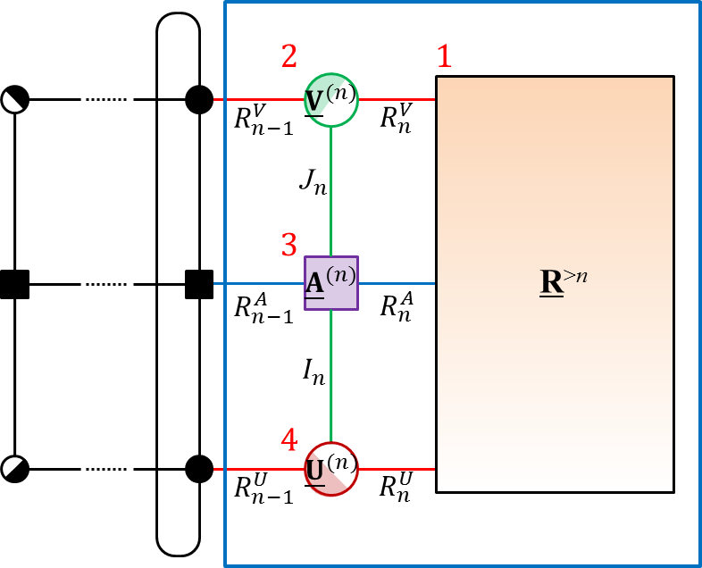
Figure 10: Iterative computation of the right tensor $\underline{\mathbf{R}}^{>n-1}$ by the contraction of the tensors $\underline{\mathbf{R}}^{>n}$, $\underline{\mathbf{V}}^{(n)}$, $\underline{\mathbf{A}}^{(n)}$, and $\underline{\mathbf{U}}^{(n)}$ during the right-to-left half sweep. The optimal order of contraction is expressed by the numbers on each tensor.

3.5 Computational Considerations

3.5.1 Initialization

The computational costs of the ALS-SVD and MALS-SVD are significantly affected by the TT-ranks of the left and right singular vectors. Even if we have good initial guesses for the left and right singular vectors $\mathbf{U}$ and $\mathbf{V}$, it may take much computational time until convergence if their TT-ranks are large. Therefore, it is advisable to initialize $\mathbf{U}$ and $\mathbf{V}$ in block TT format with relatively small TT-ranks. The minimum values of the TT-ranks are determined by

$$R^{U}_{n}=\left\lceil K/(I_{n+1}\cdots I_{N})\right\rceil,\quad R^{V}_{n}=\left\lceil K/(J_{n+1}\cdots J_{N})\right\rceil,\quad n=1,\ldots,N,$$ (65)

because each TT-core is initially left-orthogonalized and satisfies, e.g., $R^{U}_{n-1}I_{n}\geq R^{U}_{n},n=1,2,\ldots,N-1$, and the $N$th TT-core is also orthogonalized in the sense that $(\mathbf{U}^{(N)})^{\mathrm{T}}\mathbf{U}^{(N)}=\mathbf{I}_{K}$, and it must satisfy $R^{U}_{N-1}I_{N}\geq K$. Since both the ALS-SVD and MALS-SVD can adaptively determine TT-ranks during iteration process when $K\geq 2$, they update the singular vectors very fast for the first a few sweeps and usually make good initial updates for themselves.

3.5.2 Stopping Criterion

The ALS-SVD and MALS-SVD algorithms can terminate if the relative residual decreases below a prescribed tolerance parameter $\epsilon$:

$$r=\frac{\|\mathbf{A}^{\mathrm{T}}\mathbf{U}-\mathbf{V\Sigma}\|_{\mathrm{F}}}{\|\mathbf{\Sigma}\|_{\mathrm{F}}}<\epsilon.$$ (66)

The computational cost for computing $r$ is proportional to the order $N$ [34]. However, since the product $\mathbf{A}^{\mathrm{T}}\mathbf{U}$ increases the TT-ranks to the multiplications, $\{R^{A}_{n}R^{U}_{n}\}$, we perform the truncation method, called TT-rounding, proposed in [34].

3.5.3 Truncation Parameter

At each iteration, the $\delta$-truncated SVD is used to determine close to optimal TT-ranks and simultaneously to orthogonalize TT-cores. The $\delta$ value significantly affects the convergence rate of the ALS-SVD and MALS-SVD algorithms. If $\delta$ is small, then the algorithms usually converge fast within one or two full sweeps, but the TT-ranks may also grow largely, which causes high computational costs. In [18], it was reported that a MALS-based algorithm often resulted in a rapidly increasing TT-ranks during iteration process. On the other hand, if $\delta$ is large, TT-ranks grow slowly, but the algorithms may not converge to the desired accuracy but converge to a local minimum.

In this paper, we initially set the $\delta$ value to $\delta_{0}=\epsilon/\sqrt{N-1}$ in numerical simulations. In [34], it was shown that the $\delta_{0}$ yields a guaranteed accuracy in approximation and truncation algorithms. In the numerical simulations, we observed that the TT-based algorithms including the proposed algorithms converged to the desired accuracy $\epsilon$ within 1 to 3 full sweeps in most of the cases.

In the case that the algorithm could not converge to the desired tolerance $\epsilon$ after the $N_{sweep}$ number of full sweeps, we restart the algorithm with different random initializations. In this case, the $\delta$ value may not be changed or decreased to, e.g., $0.1\delta$. If $K$ is not small, the algorithms usually converge in 1 or 2 full sweeps, so a small $N_{sweep}$ value is often sufficient. But if $K$ is small, e.g., $K=2$, then the rank growth in each sweep is relatively slow and a more number of sweeps may be necessary. Moreover, in order to reduce the computational complexity, we used a rather large $\delta$ value at the first half sweep, for instance, $100\delta$. In this way, we can speed up the computation while not harming the convergence.

4 Numerical simulations

In numerical simulations, we computed the $K$ dominant singular values and correponding singular vectors of several different types of very large-scale matrices. We compared the following SVD methods including two standard methods, LOBPCG and SVDS.

1. LOBPCG: The LOBPCG [23] method can compute the $K$ largest or smallest eigenvalues of Hermitian matrices. We applied a MATLAB version of LOBPCG to the matrix $\begin{bmatrix}\mathbf{0}&\mathbf{A}\\ \mathbf{A}^{\mathrm{T}}&\mathbf{0}\end{bmatrix}$ to compute its $K$ largest eigenvalues $\mathbf{\Lambda}=\mathbf{\Sigma}=\text{diag}(\sigma_{1},\ldots,\sigma_{K})$ and the corresponding eigenvectors $\mathbf{W}=2^{-1/2}\begin{bmatrix}\mathbf{U}^{\mathrm{T}}&\mathbf{V}^{\mathrm{T}}\end{bmatrix}$.

2. SVDS: The MATLAB function SVDS computes a few singular values and vectors of matrices by using the MATLAB function EIGS, which applies the Fortran package ARPACK [30]. We applied the function EIGS directly to the matrix $\begin{bmatrix}\mathbf{0}&\mathbf{A}\\ \mathbf{A}^{\mathrm{T}}&\mathbf{0}\end{bmatrix}$, so that the matrix-by-vector products are performed more efficiently than in SVDS. We obtained its $2K$ eigenvalues/vectors of largest magnitudes, which are plus/minus largest singular values of $\mathbf{A}$: $\pm\sigma_{1},\ldots,\pm\sigma_{K}$. And then we selected only the $K$ largest singular values among them.

3. ALS-SVD, MALS-SVD: The ALS-SVD and MALS-SVD algorithms are described in Algorithms 1 and 2. For the local optimization at each iteration, we applied the MATLAB function EIGS with the projected matrix-by-vector product described in Section 3.3. We computed $2K$ eigenvalues/vectors of largest magnitudes, $\pm\sigma_{1},\ldots,\pm\sigma_{K}$, at each local optimization as described in the SVDS method above.

4. ALS-EIG, MALS-EIG: The ALS and MALS schemes are implemented for computing the $K$ largest eigenvalues of the Hermitian matrix $\mathbf{A}^{\mathrm{T}}\mathbf{A}$ by maximizing the block Rayleigh quotient [8]. We applied the MATLAB function EIGS for optimization at each iteration. After computing the $K$ eigenvalues of largest magnitudes $\mathbf{\Lambda}=\mathbf{\Sigma}^{2}$ and eigenvectors $\mathbf{V}$ of $\mathbf{A}^{\mathrm{T}}\mathbf{A}$, the iteration stops when

   $$\|\mathbf{A}^{\mathrm{T}}\mathbf{AV\Sigma}^{\dagger}-\mathbf{V\Sigma}\|^{2}<\epsilon^{2}\|\mathbf{\Sigma}\|^{2},$$ (67)

   where $\mathbf{\Sigma}^{\dagger}$ is the pseudo-inverse. The left singular vectors are computed by $\mathbf{U}=\mathbf{AV\Sigma}^{-1}$ if $\mathbf{\Sigma}$ is invertible. If $\mathbf{\Sigma}$ is not invertible, then eigenvalue decomposition of $\mathbf{AA}^{\mathrm{T}}$ is computed to obtain $\mathbf{U}$. In this way, the relative residual can be controlled below $\epsilon$ as

   $$\begin{split}\|\mathbf{A}^{\mathrm{T}}\mathbf{U}-\mathbf{V\Sigma}\|^{2}&=\|\mathbf{A}^{\mathrm{T}}\mathbf{AV\Sigma}^{-1}-\mathbf{V\Sigma}\|^{2}\leq\epsilon^{2}\|\mathbf{\Sigma}\|^{2}.\end{split}$$ (68)

We note that the computation of $\mathbf{A}^{\mathrm{T}}\mathbf{A}$ and $\mathbf{U}=\mathbf{AV\Sigma}^{-1}$ is followed by the truncation algorithm of [34] to reduce the TT-ranks. Especially, the computational cost for the truncation of $\mathbf{A}^{\mathrm{T}}\mathbf{A}$ is $\mathcal{O}(NIR_{A}^{6})$, which is quite large compared to the computational costs of the ALS-SVD and MALS-SVD in Table 1. Moreover, for the two standard methods, LOBPCG and SVDS, the matrix $\mathbf{A}$ is in full matrix format, whereas for the block TT-based SVD methods, the matrix $\mathbf{A}$ is in matrix TT format. In the simulations, we stopped running the two standard methods when the size of the matrix grows larger than $2^{13}\times 2^{13}$, because not only the computational time is high, but also the storage cost exceed the desktop memory capacity.

We implemented our code in MATLAB. The simulations were performed on a desktop computer with Intel Core i7 X 980 CPU at 3.33 GHz and 24GB of memory running Windows 7 Professional and MATLAB R2007b. In the simulations, we performed 30 repeated experiments independently and averaged the results.

4.1 Random Matrix with Prescribed Singular Values

In order to measure the accuracy of computed singular values, we built matrices of rank 25 in matrix TT format by

$$\mathbf{A}=\mathbf{U}_{0}\mathbf{\Sigma}_{0}\mathbf{V}_{0}^{\mathrm{T}}\in\mathbb{R}^{2^{N}\times 2^{N}},$$ (69)

where $\mathbf{U}_{0}\in\mathbb{R}^{2^{N}\times 25}$ and $\mathbf{V}_{0}\in\mathbb{R}^{2^{N}\times 25}$ are left and right singular vectors in block-$N$ TT format, where each of TT-cores are generated by standard normal distribution and then orthogonalized to have orthonormal column vectors in $\mathbf{U}_{0}$ and $\mathbf{V}_{0}$. The singular values $\mathbf{\Sigma}_{0}=\text{diag}(\sigma^{0}_{1},\sigma^{0}_{2},\ldots,\sigma^{0}_{25})$ are given by

$$\sigma^{0}_{k}=\beta^{k-1},\ k=1,2,\ldots,25.$$ (70)

The $\beta$ takes values from $\{0.2,0.3,0.4,0.5,0.6\}$. Figure 11 illustrates the 25 singular values for each $\beta$ value. The block TT-ranks of $\mathbf{U}_{0}$ and $\mathbf{V}_{0}$ are set at the fixed value $5$. The TT-cores of $\mathbf{A}$ in (69) were calculated based on the TT-cores of $\mathbf{U}_{0}$ and $\mathbf{V}_{0}$ as

$$\begin{split}\mathbf{A}^{(n)}_{:,i_{n},j_{n},:}&=\mathbf{U}^{(n)}_{:,i_{n},:}\otimes\mathbf{V}^{(n)}_{:,j_{n},:}\in\mathbb{R}^{R^{U}_{n-1}R^{V}_{n-1}\times R^{U}_{n}R^{V}_{n}},\quad n=1,2,\ldots,N-1,\\ \mathbf{A}^{(N)}_{:,i_{N},j_{N},:}&=\sum_{k=1}^{25}\mathbf{U}^{(N)}_{:,k,i_{N},:}\otimes\mathbf{V}^{(N)}_{:,k,j_{N},:}\in\mathbb{R}^{R^{U}_{N-1}R^{V}_{N-1}\times R^{U}_{N}R^{V}_{N}},\end{split}$$ (71)

for $i_{n}=1,\ldots,I_{n},j_{n}=1,\ldots,J_{n}.$ We set $\epsilon=10^{-8}$ and $K=10$. The relative error for the estimated singular values $\mathbf{\Sigma}$ is calculated by

$$\frac{\|\mathbf{\Sigma}-\mathbf{\Sigma}_{0}\|_{\mathrm{F}}}{\|\mathbf{\Sigma}_{0}\|_{\mathrm{F}}}.$$ (72)

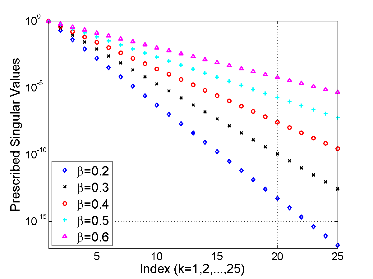
Figure 11: Singular values of the random matrices for Section 4.1

Figure 12 shows the convergence of the proposed ALS-SVD and MALS-SVD algorithms for different $K$ values, $K=2,10$, fixed dimension $N=50$, and truncation parameter $\delta=10^{-8}/\sqrt{N-1}$. In Figures 12(a) and (b), the value $K=2$ is relatively small. In this case, the maximum of the TT-ranks of the right singular vectors $\mathbf{U}$ increases slowly in Figure 12(b). The convergence of the MALS-SVD is faster than the ALS-SVD in Figure 12(a), because its TT-ranks increases faster than the ALS-SVD. Note that the relatively fast convergence of the MALS-SVD for small $K$ values were explained in the inequality (48). On the other hand, Figures 12(c) and (d) show the results when the $K$ value is relatively large, i.e., $K=10$. In Figure 12(d), the TT-ranks of $\mathbf{U}$ increase fastly in a few initial iterations, and then decrease to the optimal TT-ranks a few iterations before the convergence. In this case, we can see that both the ALS-SVD and MALS-SVD converge fastly in Figure 12(c). Note that the fast convergence does not imply small computational costs because the large TT-ranks will slow the speed of computation at each iteration.

(a)	(b)
(c)	(d)

Figure 12: Convergence of the ALS-SVD and MALS-SVD algorithms for the dimension $N=50$ for Section 4.1. Top panels (a) and (b) are the results for $K=2$ and the bottom panels (c) and (d) are the results for $K=10$. Circles represent the end of the right-to-left half sweep, and the squares represent each of the full-sweeps.

In Figure 13, we can see that the computational costs of the TT-based algorithms grow only logarithmically with the matrix size, whereas the times for the standard SVD algorithms grow exponentially with $N$. Among the TT-based algorithms, the ALS-SVD and MALS-SVD show the smallest computational costs. The ALS-EIG and MALS-EIG have higher computational costs because the product $\mathbf{A}^{\mathrm{T}}\mathbf{A}$ increases its matrix TT-ranks and the subsequent truncation step results in high computational costs. The LOBPCG and SVDS show a fast rate of increase in the computational cost. The LOBPCG and SVDS were stopped running for larger matrix sizes than $2^{13}\times 2^{13}$ because of the computational cost and desktop computer memory capacity. The black dotted line shows a predicted computational time for the LOBPCG.

Moreover, the ALS-based methods are faster than the MALS-based methods because the MALS-based methods solve larger optimization problems at each iteration over the merged TT-cores. However, the MALS-based methods can determine TT-ranks during iteration even if $K=1$, and the rate of convergence per iteration is faster for small $K$ values as shown in Figure 12.

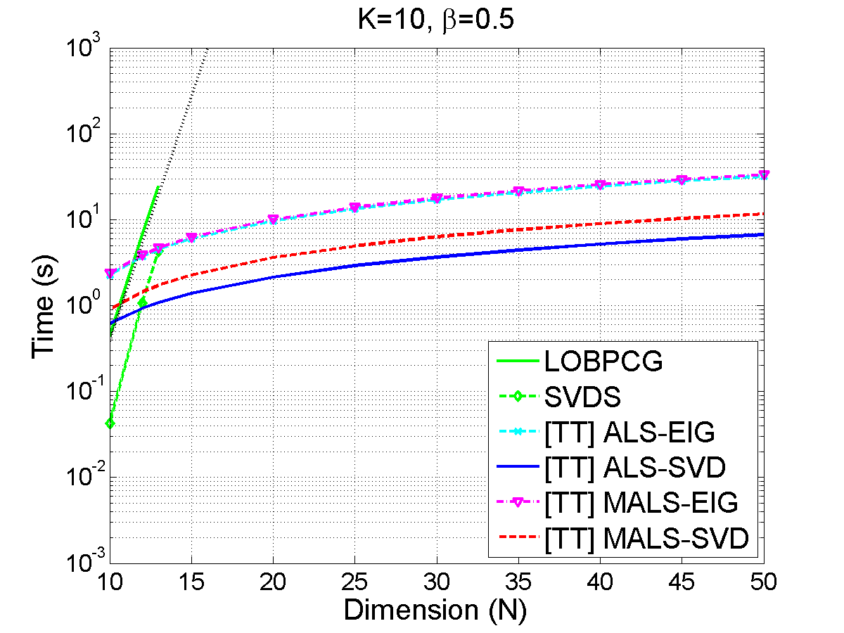
Figure 13: Performances for $2^{N}\times 2^{N}$ random matrices with $10\leq N\leq 50$ and fixed $\beta=0.5$

Figure 14 shows the performances of the four TT-based algorithms for various $\beta$ values for the random matrices $\mathbf{A}\in\mathbb{R}^{2^{N}\times 2^{N}}$ with $N=50$. In Figure 14(a), the ALS-SVD and MALS-SVD show the smallest computational times over all the $\beta$ values. In Figures 14(b) and (c), we can see that the ALS-SVD and MALS-SVD accurately estimate the block TT-ranks and the $K=10$ dominant singular values. On the other hand, the ALS-EIG and MALS-EIG estimate the block TT-ranks and the singular values slightly less accurately, especially for small $\beta$ values. We note that the ALS-EIG and MALS-EIG take square roots on the obtained eigenvalues to compute the singular values.

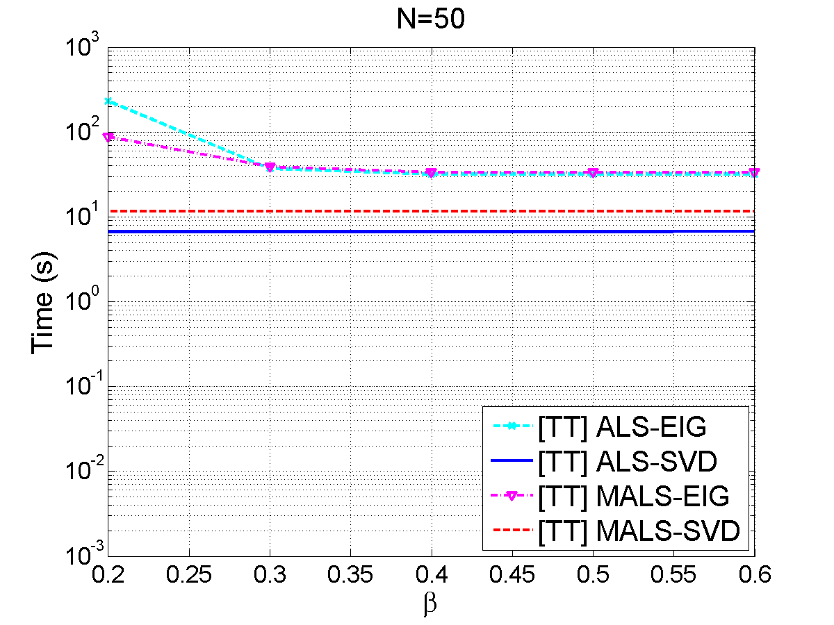
(a)	(b)
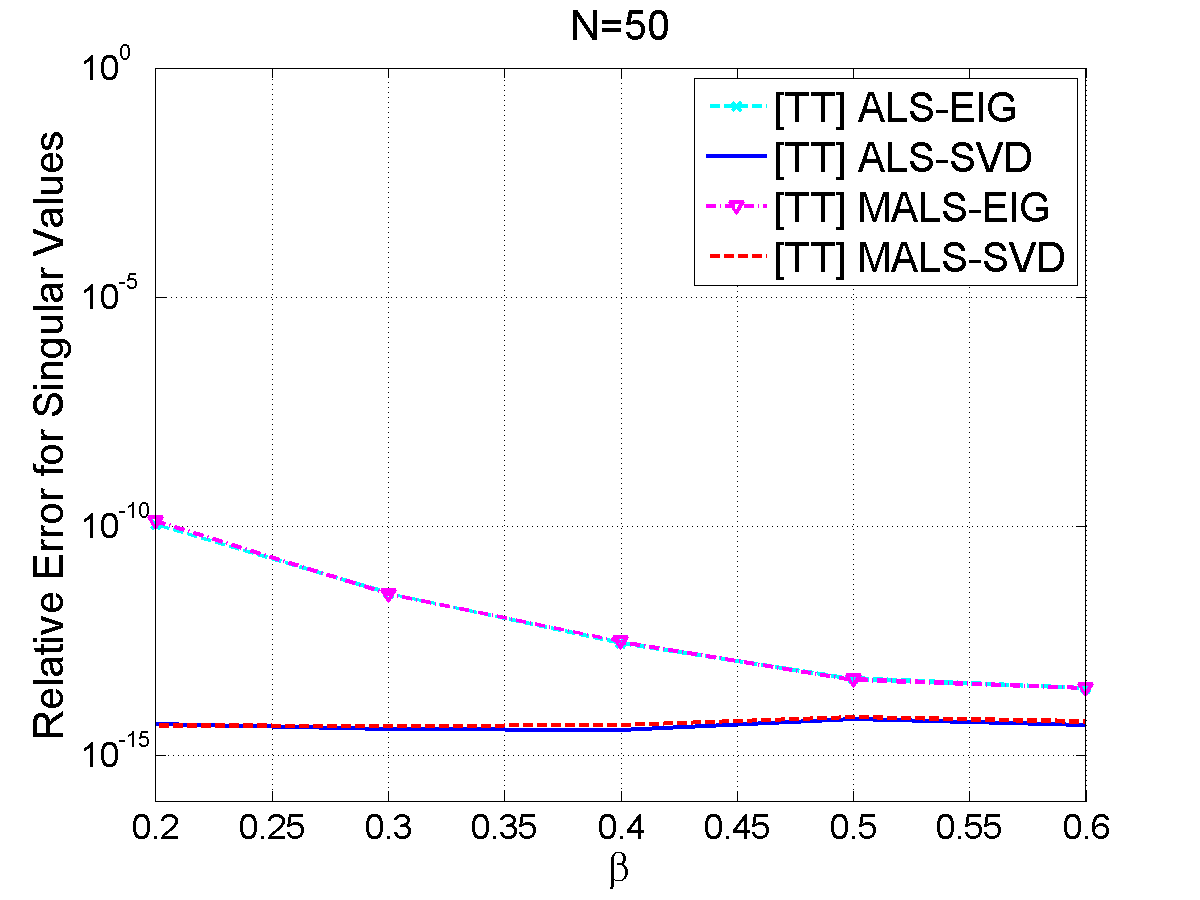
(c)

Figure 14: Performances for $2^{N}\times 2^{N}$ random matrices with prescribed singular values for $N=50$ and various $\beta$ values. (a) The computational time, (b) maximum block TT-rank of right singular vectors, and (c) relative error for singular values.

4.2 A Submatrix of Hilbert Matrix

The Hilbert matrix $\mathbf{H}\in\mathbb{R}^{P\times P}$ is a symmetric matrix with entries $h_{i,j}=(i+j-1)^{-1},i,j=1,2,\ldots,P$. It is known that the eigenvalues of the Hilbert matrix decay to zero very fast. In this simulation, we consider a rectangular submatrix $\mathbf{A}\in\mathbb{R}^{2^{N}\times 2^{N-1}}$ of the Hilbert matrix defined by

$$\mathbf{A}=\mathbf{H}(:,1:2^{N-1})\in\mathbb{R}^{2^{N}\times 2^{N-1}}$$ (73)

in MATLAB notation, in order to apply the SVD algorithms to the non-symmetric matrix $\mathbf{A}$. The matrix TT representation of $\mathbf{A}$ was computed based on the explicit TT representation of Hankel matrices, which is described in Appendix B in detail. For this purpose, we applied the cross approximation algorithm FUNCRS2 in TT-Toolbox [35] to transform the vector $[1,1,2^{-1},3^{-1},\ldots,(2^{N+1}-1)^{-1}]^{\mathrm{T}}\in\mathbb{R}^{2^{N+1}}$ to a vector TT format with the relative approximation error of $10^{-8}$. Then we used the explicit TT representation of Hankel matrices to convert the vector into the Hilbert matrix in matrix TT format. Finally, we could find that the maximum value of the matrix TT-ranks, $\text{max}(R^{A}_{n})$, are between 14 and 22 over $10\leq N\leq 50$.

For comparison of performances of the SVD algorithms, we set $\epsilon=10^{-3}$ and $K=10$. In Figure 15(a), the computational costs of the TT-based algorithms grow logarithmically with the matrix size. The ALS-SVD and MALS-SVD have the least computational costs. In Figure 15(b), we can see that the maximum block TT-ranks, $\text{max}(R^{V}_{n})$, are relatively large for $N=30,40,50$, which may have affected the computational costs in Figure 15(a).

(a)	(b)

Figure 15: Performances for the $2^{N}\times 2^{N-1}$ submatrices of Hilbert matrices with $10\leq N\leq 50$ and $K=10$. (a) Computational cost and (b) maximum block TT-rank of the right singular vectors.

4.3 Random Tridiagonal Matrix

A tridiagonal matrix is a banded matrix whose nonzero entries are only on the main diagonal, the first diagonal above the main diagonal, and the first diagonal below the main diagonal. The matrix TT representation of a tridiagonal matrix is described in Appendix C. We randomly generated three vector TT tensors $\mathbf{a},\mathbf{b},\mathbf{c}$ with TT-cores drawn from the standard normal distribution and TT-ranks $R_{n}=R=5,1\leq n\leq N-1$. Then, each TT-cores are orthogonalized to yield $\|\mathbf{a}\|=\|\mathbf{b}\|=\|\mathbf{c}\|=1$. We built the $2^{N}\times 2^{N}$ tridiagonal matrix $\mathbf{A}$ whose sub, main, and super diagonals are $\mathbf{a},\mathbf{b},$ and $\mathbf{c}$. The matrix TT-ranks of $\mathbf{A}$ are bounded by $5R$, which are largely reduced after truncation to around 17.

For performance evaluation, we set $\epsilon=10^{-8}$ and $K=10$. In this simulation, all the TT-based SVD algorithms converged within 3 full sweeps.

Figure 16(a) shows that the computational costs for the TT-based SVD algorithms are growing logarithmically with the matrix size over $10\leq N\leq 50$. The ALS-SVD and MALS-SVD have the smallest computational costs. The ALS-EIG and MALS-EIG have relatively high computational costs because the matrix TT-ranks are relatively large in this case so the truncation of $\mathbf{A}^{\mathrm{T}}\mathbf{A}$ was computationally costly. Figure 16(b) shows that the maximum value of the block TT-ranks, $\text{max}(R^{V}_{n})$, are bounded by 20 and slowly decreasing as $N$ increases. We note that the diagonal entries of the matrices were randomly generated and the 10 dominant singular values were close to each other, similarly as the identity matrix. We conclude that the TT-based SVD algorithms can accurately compute several dominant singular values and singular vectors even in the case that the singular values are almost identical.

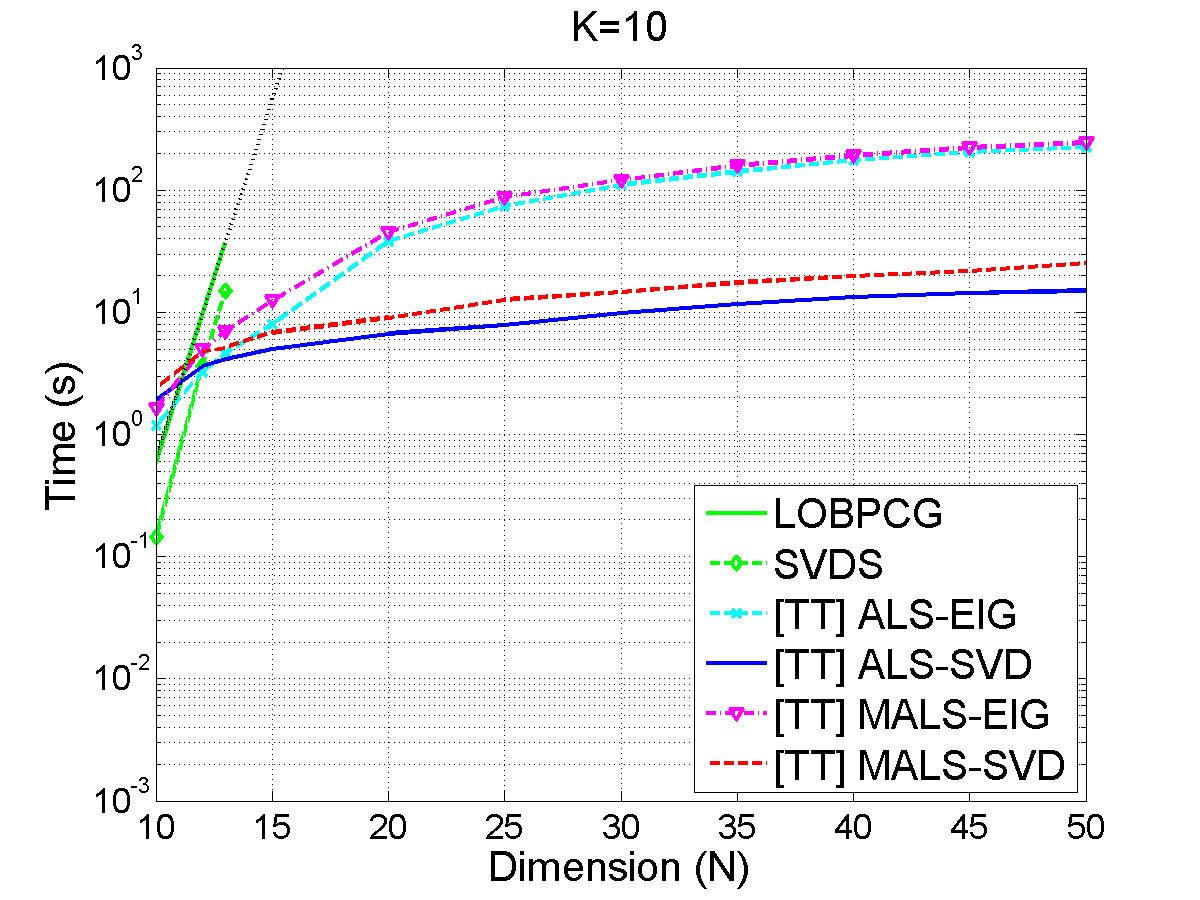
(a)	(b)

Figure 16: Performances for the $2^{N}\times 2^{N}$ random tridiagonal matrices with $K=10$ and $10\leq N\leq 50$. (a) Computational cost and (b) maximum block TT-rank of the right singular vectors.

4.4 Random Toeplitz Matrix

Toeplitz matrix is a square matrix that has constant diagonals. An explicit matrix TT representation of a Toeplitz matrix is described in [21]. See Appendix B for more detail. We generated a vector $\mathbf{x}=[x_{1},\ldots,x_{2^{N+1}}]^{\mathrm{T}}$ in vector TT format with its TT-cores drawn from the standard normal distribution and fixed TT-ranks $R_{n}=R=5$. Then, we converted $\mathbf{x}$ into a Toeplitz matrix $\mathbf{A}\in\mathbb{R}^{2^{N}\times 2^{N}}$ in matrix TT format with entries

$$a_{i,j}=x_{2^{N}+i-j},\quad i,j=1,2,\ldots,2^{N}.$$ (74)

The matrix TT-ranks of $\mathbf{A}$ are bounded by twice the TT-ranks of $\mathbf{x}$, i.e., $2R$ [21].

Since the matrix $\mathbf{A}$ is generated randomly, we cannot expect that the TT-ranks of the left and right singular vectors are bounded over $N$. Instead, we fixed the maximum of the TT-ranks, $R_{max}$, and compared the computational times and relative residuals of the algorithms. We set $K=10$, and $N_{sweep}=2$.

Figures 17(a) and (b) show the performances of the SVD algorithms for $R_{max}=15$ and $10\leq N\leq 30$. In Figure 17(a), we can see that the computational costs of the TT-based algorithms grow logarithmically with the matrix size because the matrix TT-ranks and the block TT-ranks are bounded by $2R=10$ and $R_{max}=15$, respectively. In Figure 17(b), the relative residual values remain almost constantly around $0.15$. Figures 17(c) and (d) show the computational costs and relative residuals for various $10\leq R_{max}\leq 30$ and fixed $N=30$. We can see that the computational cost for the ALS-SVD is the smallest and growing slowly as $R_{max}$ increases.

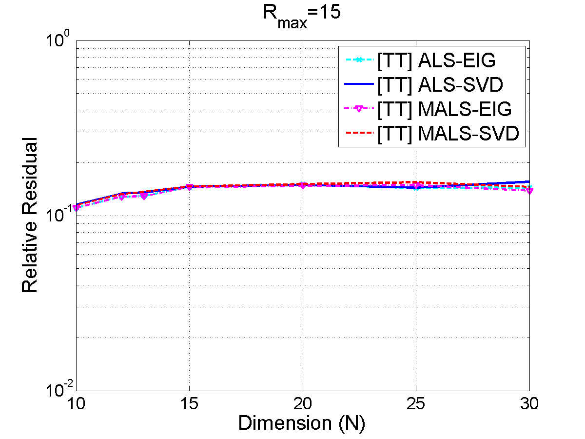
(a)	(b)
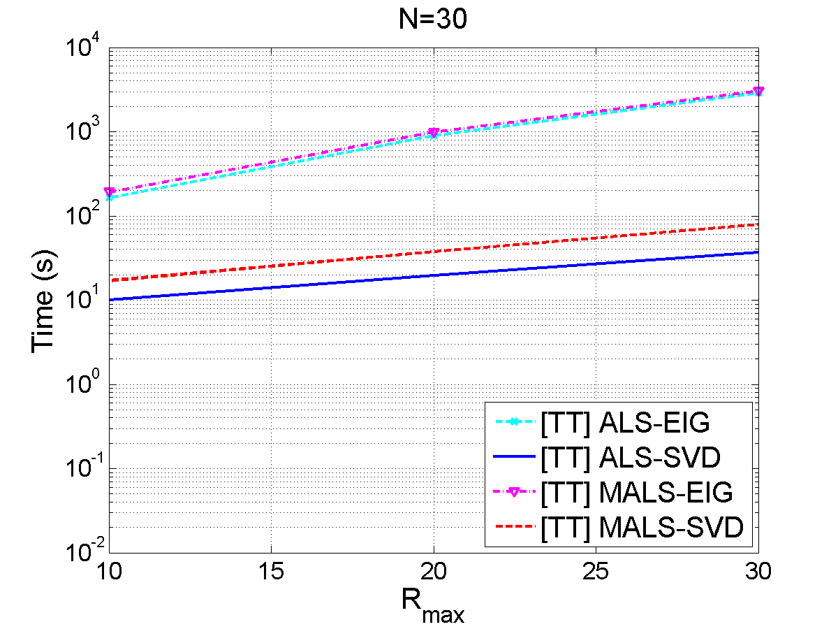
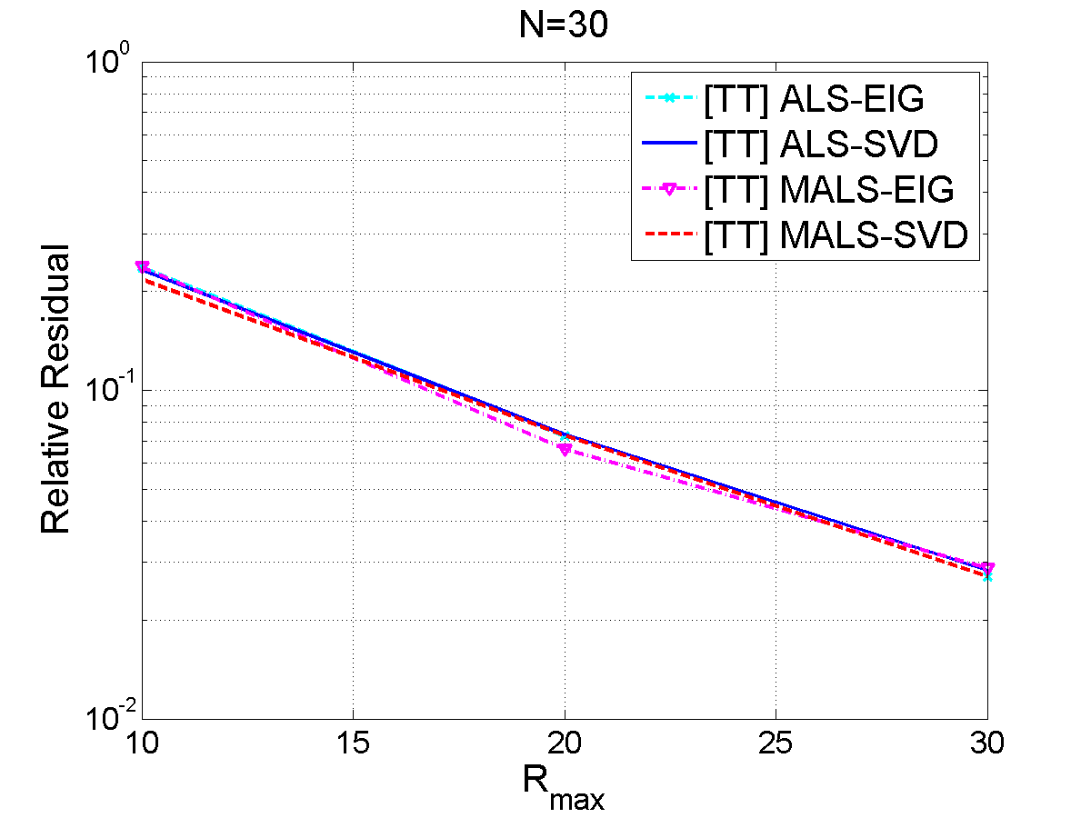
(c)	(d)

Figure 17: Performances for $2^{N}\times 2^{N}$ random Toeplitz matrices. The block TT-ranks of the left and right singular vectors are bounded by $R_{max}$. (a) Computational cost and (b) relative residual for fixed $R_{max}=15$ and various $10\leq N\leq 30$. (c) Computational cost and (b) relative residual for various $10\leq R_{max}\leq 30$ and fixed $N=30$.

5 Conclusion and Discussions

In this paper, we proposed new SVD algorithms for very large-scale structured matrices based on TT decompositions. Unlike previous researches focusing only on eigenvalue decomposition (EVD) of symmetric positive semidefinite matrices [8, 19, 20, 22, 25, 28, 33, 40], the proposed algorithms do not assume symmetricity of the data matrix $\mathbf{A}$. We investigated the computational complexity of the proposed algorithms rigorously, and provided optimized ways of tensor contractions for the fast computation of the singular values. We conducted extensive simulations to demonstrate the effectiveness of the proposed SVD algorithms compared with the other TT-based algorithms which are based on the EVD of symmetric positive semidefinite matrices.

Once a very large-scale matrix is represented in matrix TT format, the proposed ALS-SVD and MALS-SVD algorithms can compute the SVD in logarithmic time complexity with respect to the matrix size under the assumption that the TT-ranks are bounded. Unlike the EVD-based methods, the proposed algorithms avoid truncation of the matrix TT-ranks of the product $\mathbf{A}^{\mathrm{T}}\mathbf{A}$ but directly optimize the maximization problem (1). In the simulated experiments, we demonstrated that the computational costs of the EVD-based algorithms are highly affected by the matrix TT-ranks, and the proposed methods are highly competitive compared with the EVD-based algorithms. Moreover, we showed that the proposed methods can compute the SVD of $2^{50}\times 2^{50}$ matrices accurately even in a few seconds on desktop computers.

The proposed SVD methods can compute a few dominant singular values and corresponding singular vectors of TT-structured matrices. The structured matrices used in the simulations are random matrices with prescribed singular values, Hilbert matrix, random tridiagonal matrix, and random Toeplitz matrix. The singular vectors are represented as block TT formats, and the TT-ranks are adaptively determined during iteration process. Moreover, we also presented the case of random Toeplitz matrices, where the block TT-ranks of the singular vectors are not bounded as the matrix size increases. In this case, the proposed methods computed approximate solutions based on fixed TT-ranks with reasonable approximation errors. Since the TT-ranks are fixed, the computational cost will be much reduced if the $\delta$-truncated SVD step is replaced with the QR decomposition.

In the simulated experiments, we observed that the truncation parameter $\delta$ for the $\delta$-trucated SVD highly affects the convergence. If $\delta$ is too large, then the algorithm falls into local minimum and its accuracy does not improve any more. If $\delta$ is too small, then the TT-ranks grow fastly and the computational cost increases. We initialized the $\delta$ value by $\delta_{0}=\epsilon/\sqrt{N-1}$ as proposed by Oseledets [34], in which case the proposed algorithms usually achieved the desired accuracy. If the TT-based ALS and MALS algorithms fall into local minimum, we restarted the algorithms with new initial block TT tensors. If a proper $\delta$ value is selected and the number $K$ of singular values is large enough, then the algorithms converge usually in at most 3 full sweeps. Moreover, the MALS algorithm shows faster convergence than the ALS algorithm because the TT-ranks can be increased more fastly at each iteration.

The performance of the TT-based algorithms are highly dependent on the choice of the optimization algorithms for solving the reduced local problems. In the simulations we applied the MATLAB function EIGS to the matrix $\begin{bmatrix}\mathbf{0}&\mathbf{A}\\ \mathbf{A}^{\mathrm{T}}&\mathbf{0}\end{bmatrix}$ in order to obtain accurate singular values.

In order to convert a very large-scale matrix into matrix TT format, it is suggested to employ cross approximation methods [1, 38]. We also applied the MATLAB function FUNCRS2 in TT-Toolbox [35] for Hilbert matrices in the numerical simulations.

The proposed algorithms rely on the optimization with the trace function described in the maximization problem (1), so they cannot be applied for computing $K$ smallest singular values directly. In Appendix A, we explained how the $K$ smallest singular values and corresponding singular vectors can be computed by using the EVD-based algorithms. In the future work, we will develop a more efficient method for computing a few smallest singular values and corresponding singular vectors based on TT decompositions.

Appendix A Optimization Problems for Extremal Singular Values

The SVD of a matrix $\mathbf{A}\in\mathbb{R}^{P\times Q}$ is closely related to the eigenvalue decomposition (EVD) of the following $(P+Q)\times(P+Q)$ matrix

$$\mathbf{B}=\begin{bmatrix}\mathbf{0}&\mathbf{A}\\ \mathbf{A}^{\mathrm{T}}&\mathbf{0}\end{bmatrix}.$$ (75)

In this section, we show the relationship between the EVD optimization problems of $\mathbf{B}$ and the SVD optimization problems of $\mathbf{A}$.

A.1 Eigenvalues of $\mathbf{B}$

We assume that $P\geq Q$. The SVD of the matrix $\mathbf{A}\in\mathbb{R}^{P\times Q}$ can be expressed as

$$\mathbf{A}=\begin{bmatrix}\mathbf{U}_{0}&\mathbf{U}_{0}^{\bot}\end{bmatrix}\begin{bmatrix}\mathbf{\Sigma}_{0}\\ \mathbf{0}\end{bmatrix}\mathbf{V}_{0}^{\mathrm{T}},$$ (76)

where $\mathbf{U}_{0}\in\mathbb{R}^{P\times Q}$, $\mathbf{U}_{0}^{\bot}\in\mathbb{R}^{P\times(P-Q)}$, and $\mathbf{V}_{0}\in\mathbb{R}^{Q\times Q}$ are the matrices of singular vectors and $\mathbf{\Sigma}_{0}\in\mathbb{R}^{Q\times Q}$ is the diagonal matrix with nonnegative diagonal entries $\sigma_{1}\geq\sigma_{2}\geq\cdots\geq\sigma_{Q}$.

Lemma A.1.

The EVD of the matrix $\mathbf{B}$ can be written by

$$\mathbf{B}=\mathbf{W}_{0}\mathbf{\Lambda}_{0}\mathbf{W}_{0}^{\mathrm{T}},$$ (77)

where

$$\mathbf{W}_{0}=\frac{1}{\sqrt{2}}\begin{bmatrix}\mathbf{U}_{0}&\mathbf{U}_{0}&\sqrt{2}\mathbf{U}_{0}^{\bot}\\ \mathbf{V}_{0}&-\mathbf{V}_{0}&\mathbf{0}\end{bmatrix}\in\mathbb{R}^{(P+Q)\times(P+Q)},$$ (78)

$$\mathbf{\Lambda}_{0}=\begin{bmatrix}\mathbf{\Sigma}_{0}&&\\ &-\mathbf{\Sigma}_{0}&\\ &&\mathbf{0}\end{bmatrix}\in\mathbb{R}^{(P+Q)\times(P+Q)}.$$ (79)

Proof.

We can compute that $\mathbf{W}_{0}^{\mathrm{T}}\mathbf{W}_{0}=\mathbf{I}_{P+Q}$. We can show that $\mathbf{BW}_{0}=\mathbf{W}_{0}\mathbf{\Lambda}_{0}$. ∎

We can conclude that the eigenvalues of the matrix $\mathbf{B}$ consist of $\pm\sigma_{1},\pm\sigma_{2},\ldots,\pm\sigma_{Q}$, and an extra zero of multiplicity $P-Q$.

A.2 Maximal Singular Values

The $K$ largest eigenvalues of the matrix $\mathbf{B}$ can be computed by solving the trace maximization problem [12, Theorem 1]

$$\begin{split}\mathop{\text{maximize}}_{\mathbf{W}}&\qquad\text{trace}\left(\mathbf{W}^{\mathrm{T}}\mathbf{B}\mathbf{W}\right)\\ \text{subject to}&\qquad\mathbf{W}^{\mathrm{T}}\mathbf{W}=\mathbf{I}_{K}.\end{split}$$ (80)

Instead of building the matrix $\mathbf{B}$ explicitly, we solve the equivalent maximization problem described as follows.

Proposition A.2.

For $K\leq Q$, the maximization problem (80) is equivalent to

$$\begin{split}\mathop{\text{maximize}}_{\mathbf{U},\mathbf{V}}&\qquad\text{trace}\left(\mathbf{U}^{\mathrm{T}}\mathbf{A}\mathbf{V}\right)\\ \text{subject to}&\qquad\mathbf{U}^{\mathrm{T}}\mathbf{U}=\mathbf{V}^{\mathrm{T}}\mathbf{V}=\mathbf{I}_{K}.\end{split}$$ (81)

Proof.

Let

$$\mathbf{W}=\frac{1}{\sqrt{2}}\begin{bmatrix}\mathbf{U}\\ \mathbf{V}\end{bmatrix}\in\mathbb{R}^{(P+Q)\times K},$$ (82)

then

$$\text{trace}\left(\mathbf{W}^{\mathrm{T}}\mathbf{B}\mathbf{W}\right)=\text{trace}\left(\mathbf{U}^{\mathrm{T}}\mathbf{AV}\right).$$ (83)

First, we can show that

$$\max_{\mathbf{W}^{\mathrm{T}}\mathbf{W}=\mathbf{I}_{K}}\text{trace}\left(\mathbf{W}^{\mathrm{T}}\mathbf{B}\mathbf{W}\right)\geq\max_{\mathbf{U}^{\mathrm{T}}\mathbf{U}=\mathbf{V}^{\mathrm{T}}\mathbf{V}=\mathbf{I}_{K}}\text{trace}\left(\mathbf{U}^{\mathrm{T}}\mathbf{AV}\right).$$ (84)

Next, we can show that the maximum value $\sigma_{1}+\sigma_{2}+\cdots+\sigma_{K}$ of $\text{trace}\left(\mathbf{W}^{\mathrm{T}}\mathbf{B}\mathbf{W}\right)$ is obtained by $\text{trace}\left(\mathbf{U}^{\mathrm{T}}\mathbf{AV}\right)$ when $\mathbf{U}$ and $\mathbf{V}$ are equal to the first $K$ singular vectors of $\mathbf{U}_{0}$ and $\mathbf{V}_{0}$. ∎

A.3 Minimal Singular Values

Suppose that $P=Q$. The $K$ minimal singular values of $\mathbf{A}$ can be obtained by computing $2K$ eigenvalues of $\mathbf{B}$ with the smallest magnitudes, that is, $\pm\sigma_{Q-K+1},\pm\sigma_{Q-K+2},\ldots,\pm\sigma_{Q}$. Computing the $2K$ eigenvalues of $\mathbf{B}$ with the smallest magnitudes can be formulated by the following trace minimization problem

$$\begin{split}\mathop{\text{minimize}}_{\mathbf{W}}&\qquad\text{trace}\left(\mathbf{W}^{\mathrm{T}}\mathbf{B}^{2}\mathbf{W}\right)\\ \text{subject to}&\qquad\mathbf{W}^{\mathrm{T}}\mathbf{W}=\mathbf{I}_{2K}.\end{split}$$ (85)

We can translate the above minimization problem into the equivalent minimization problem without building the matrix $\mathbf{B}$ explicitly as follows.

Proposition A.3.

The minimization problem (85) is equivalent to the following two minimization problems if a permutation ambiguity is allowed:

$$\begin{split}\mathop{\text{minimize}}_{\mathbf{V}}&\qquad\text{trace}\left(\mathbf{V}^{\mathrm{T}}\mathbf{A}^{\mathrm{T}}\mathbf{A}\mathbf{V}\right)\\ \text{subject to}&\qquad\mathbf{V}^{\mathrm{T}}\mathbf{V}=\mathbf{I}_{K}\end{split}$$ (86)

and

$$\begin{split}\mathop{\text{minimize}}_{\mathbf{U}}&\qquad\text{trace}\left(\mathbf{U}^{\mathrm{T}}\mathbf{AA}^{\mathrm{T}}\mathbf{U}\right)\\ \text{subject to}&\qquad\mathbf{U}^{\mathrm{T}}\mathbf{U}=\mathbf{I}_{K}.\end{split}$$ (87)

That is, the $K$ minimal singular values of $\mathbf{A}$ can be computed by applying the eigenvalue decomposition for $\mathbf{A}^{\mathrm{T}}\mathbf{A}$ and $\mathbf{A}\mathbf{A}^{\mathrm{T}}$.

Proof.

Let

$$\mathbf{W}=\frac{1}{\sqrt{2}}\begin{bmatrix}\mathbf{U}&\mathbf{U}\\ \mathbf{V}&-\mathbf{V}\end{bmatrix}\in\mathbb{R}^{(P+Q)\times 2K},$$ (88)

then we have

$$\text{trace}\left(\mathbf{W}^{\mathrm{T}}\mathbf{B}^{2}\mathbf{W}\right)=\text{trace}\left(\mathbf{U}^{\mathrm{T}}\mathbf{AA}^{\mathrm{T}}\mathbf{U}\right)+\text{trace}\left(\mathbf{V}^{\mathrm{T}}\mathbf{A}^{\mathrm{T}}\mathbf{A}\mathbf{V}\right).$$ (89)

By algebraic manipulation, we can derive that the constraint $\mathbf{W}^{\mathrm{T}}\mathbf{W}=\mathbf{I}_{2K}$ is equivalent to $\mathbf{U}^{\mathrm{T}}\mathbf{U}=\mathbf{V}^{\mathrm{T}}\mathbf{V}=\mathbf{I}_{K}$. ∎

Appendix B Explicit Tensor Train Representation of Toeplitz Matrix and Hankel Matrix

Explicit TT representations of Toeplitz matrices are presented in [21]. In this section, we summarize some of the simplest results of [21], and extend them to Hankel matrix and rectangular submatrices.

First, we introduct the Kronecker product representation for matrix TT format. Given a matrix $\mathbf{A}\in\mathbb{R}^{I_{1}I_{2}\cdots I_{N}\times J_{1}J_{2}\cdots J_{N}}$ in matrix TT format (15), each entry of the tensor $\underline{\mathbf{A}}\in\mathbb{R}^{I_{1}\times J_{1}\times\cdots\times I_{N}\times J_{N}}$ is representedy by the sum of scalar products

$$a_{i_{1},j_{1},i_{2},j_{2},\ldots,i_{N},j_{N}}=\sum_{r^{A}_{1}=1}^{R^{A}_{1}}\sum_{r^{A}_{2}=1}^{R^{A}_{2}}\cdots\sum_{r^{A}_{N-1}=1}^{R^{A}_{N-1}}a^{(1)}_{1,i_{1},j_{1},r^{A}_{1}}a^{(2)}_{r^{A}_{1},i_{2},j_{2},r^{A}_{2}}\cdots a^{(N)}_{r^{A}_{N-1},i_{N},j_{N},1},$$ (90)

which is equal to each entry of the matrix $\mathbf{A}$, i.e., $a_{(i_{1},i_{2},\ldots,i_{N}),(j_{1},j_{2},\ldots,j_{N})}$, where $(i_{1},i_{2},\ldots,i_{N})$ is the multi-index introduced in (2). From this expression, we can derive that the matrix $\mathbf{A}$ can be represented as sums of Kronecker products of matrices

$$\mathbf{A}=\sum_{r^{A}_{1}=1}^{R^{A}_{1}}\sum_{r^{A}_{2}=1}^{R^{A}_{2}}\cdots\sum_{r^{A}_{N-1}=1}^{R^{A}_{N-1}}\mathbf{A}^{(N)}_{1,r^{A}_{N-1}}\otimes\mathbf{A}^{(N-1)}_{r^{A}_{N-1},r^{A}_{N-2}}\otimes\cdots\otimes\mathbf{A}^{(1)}_{r^{A}_{1},1},$$ (91)

where the matrices $\mathbf{A}^{(n)}_{r^{A}_{n},r^{A}_{n-1}}\in\mathbb{R}^{I_{n}\times J_{n}}$ are defined by

$$\mathbf{A}^{(n)}_{r^{A}_{n},r^{A}_{n-1}}=\left(a^{(n)}_{r^{A}_{n-1},i_{n},j_{n},r^{A}_{n}}\right)_{i_{n},j_{n}}=\underline{\mathbf{A}}^{(n)}(r^{A}_{n-1},:,:,r^{A}_{n}).$$ (92)

Note that the positions of the indices $r^{A}_{n-1}$ and $r^{A}_{n}$ have been switched for notational convenience.

Next, we present the explicit TT representations for Toeplitz matrices and Hankel matrices. The $2^{N}\times 2^{N}$ upper triangular Toeplitz matrix generated by $\left[s_{1},s_{2},\ldots,s_{2^{N}-1}\right]^{\mathrm{T}}$ is written by

$$\mathbf{T}=\begin{bmatrix}0&s_{1}&s_{2}&\cdots&s_{2^{N}-2}&s_{2^{N}-1}\\ &0&s_{1}&\cdots&s_{2^{N}-3}&s_{2^{N}-2}\\ &&&&\vdots&\vdots\\ &&&&0&s_{1}\\ &&&&&0\end{bmatrix}.$$ (93)

Similarly, the $2^{N}\times 2^{N}$ upper anti-triangular Hankel matrix generated by $\left[s_{1},s_{2},\ldots,s_{2^{N}-1}\right]^{\mathrm{T}}$ is written by

$$\mathbf{H}=\begin{bmatrix}s_{2^{N}-1}&s_{2^{N}-2}&\cdots&s_{2}&s_{1}&0\\ s_{2^{N}-2}&s_{2^{N}-3}&\cdots&s_{1}&0&\\ \vdots&\vdots&&&&\\ s_{1}&0&&&&\\ 0&&&&&\end{bmatrix}.$$ (94)

The matrix TT representation for the Toeplitz matrix is presented in the following theorem.

Theorem B.1 (An explicit matrix TT representation of Toeplitz matrix, [21]).

Let

$$\mathbf{I}=\begin{bmatrix}1&0\\ 0&1\end{bmatrix},\quad\mathbf{J}=\begin{bmatrix}0&1\\ 0&0\end{bmatrix},\quad\mathbf{K}=\begin{bmatrix}0&0\\ 1&0\end{bmatrix}$$ (95)

be $2\times 2$ matrices and let

$$\widetilde{\mathbf{L}}^{(N)}_{1}=\begin{bmatrix}\mathbf{I}&\mathbf{J}\end{bmatrix},\quad\widetilde{\mathbf{L}}^{(N-1)}_{1}=\cdots=\widetilde{\mathbf{L}}^{(2)}_{1}=\begin{bmatrix}\mathbf{I}&\mathbf{J}\\ \mathbf{0}&\mathbf{K}\end{bmatrix},\quad\widetilde{\mathbf{L}}^{(1)}_{1}=\begin{bmatrix}\mathbf{J}\\ \mathbf{K}\end{bmatrix},$$ (96)

$$\widetilde{\mathbf{L}}^{(N)}_{2}=\begin{bmatrix}\mathbf{J}&\mathbf{0}\end{bmatrix},\quad\widetilde{\mathbf{L}}^{(N-1)}_{2}=\cdots=\widetilde{\mathbf{L}}^{(2)}_{2}=\begin{bmatrix}\mathbf{J}&\mathbf{0}\\ \mathbf{K}&\mathbf{I}\end{bmatrix},\quad\widetilde{\mathbf{L}}^{(1)}_{2}=\begin{bmatrix}\mathbf{0}\\ \mathbf{I}\end{bmatrix}$$ (97)

be block matrices. For each of the block matrices $\widetilde{\mathbf{L}}^{(n)}_{k_{n}},$ $k_{n}=1,2$, we denote the $(q_{n},q_{n-1})$th block of $\widetilde{\mathbf{L}}^{(n)}_{k_{n}}$ by $\mathbf{L}^{(n)}_{q_{n},k_{n},q_{n-1}}\in\mathbb{R}^{2\times 2}$, that is,

$$\widetilde{\mathbf{L}}^{(n)}_{k_{n}}=\left[\mathbf{L}^{(n)}_{q_{n},k_{n},q_{n-1}}\right]_{q_{n},q_{n-1}},\quad k_{n}=1,2.$$ (98)

Suppose that the vector $\mathbf{s}=\left[s_{1},s_{2},\ldots,s_{2^{N}}\right]^{\mathrm{T}}$ of length $2^{N}$ is represented in TT format as

$$s_{k_{1},k_{2},\ldots,k_{N}}=\sum_{r_{1}=1}^{R_{1}}\sum_{r_{2}=1}^{R_{2}}\cdots\sum_{r_{N-1}=1}^{R_{N-1}}s^{(1)}_{1,k_{1},r_{1}}s^{(2)}_{r_{1},k_{2},r_{2}}\cdots s^{(N)}_{r_{N-1},k_{N},1}.$$ (99)

Then, the upper triangular Toeplitz matrix (93) is expressed in matrix TT format as

$$\mathbf{T}=\sum_{t_{1}=1}^{2R_{1}}\sum_{t_{2}=1}^{2R_{2}}\cdots\sum_{t_{N-1}=1}^{2R_{N-1}}\mathbf{T}^{(N)}_{1,t_{N-1}}\otimes\mathbf{T}^{(N-1)}_{t_{N-1},t_{N-2}}\otimes\cdots\otimes\mathbf{T}^{(1)}_{t_{1},1},$$ (100)

where $\mathbf{T}^{(n)}_{t_{n},t_{n-1}}\in\mathbb{R}^{2\times 2}$ are defined by

$$\mathbf{T}^{(n)}_{(r_{n},q_{n}),(r_{n-1},q_{n-1})}=\sum_{k_{n}=1}^{2}s^{(n)}_{r_{n-1},k_{n},r_{n}}\mathbf{L}^{(n)}_{q_{n},k_{n},q_{n-1}}$$ (101)

with $t_{n}=(r_{n},q_{n})$ for $n=1,2,\ldots,N.$

The matrix TT representation for Toeplitz matrices can be extended to Hankel matrices as follows.

Corollary B.2 (An explicit matrix TT representation of Hankel matrix).

Let

$$\mathbf{P}=\begin{bmatrix}0&1\\ 1&0\end{bmatrix},\quad\mathbf{Q}=\begin{bmatrix}1&0\\ 0&0\end{bmatrix},\quad\mathbf{R}=\begin{bmatrix}0&0\\ 0&1\end{bmatrix}$$ (102)

be $2\times 2$ matrices and let

$$\widetilde{\mathbf{M}}^{(N)}_{1}=\begin{bmatrix}\mathbf{P}&\mathbf{Q}\end{bmatrix},\quad\widetilde{\mathbf{M}}^{(N-1)}_{1}=\cdots=\widetilde{\mathbf{M}}^{(2)}_{1}=\begin{bmatrix}\mathbf{P}&\mathbf{Q}\\ \mathbf{0}&\mathbf{R}\end{bmatrix},\quad\widetilde{\mathbf{M}}^{(1)}_{1}=\begin{bmatrix}\mathbf{Q}\\ \mathbf{R}\end{bmatrix},$$ (103)

$$\widetilde{\mathbf{M}}^{(N)}_{2}=\begin{bmatrix}\mathbf{Q}&\mathbf{0}\end{bmatrix},\quad\widetilde{\mathbf{M}}^{(N-1)}_{2}=\cdots=\widetilde{\mathbf{M}}^{(2)}_{2}=\begin{bmatrix}\mathbf{Q}&\mathbf{0}\\ \mathbf{R}&\mathbf{P}\end{bmatrix},\quad\widetilde{\mathbf{M}}^{(1)}_{2}=\begin{bmatrix}\mathbf{0}\\ \mathbf{P}\end{bmatrix}$$ (104)

be block matrices. For each of the block matrices $\widetilde{\mathbf{M}}^{(n)}_{k_{n}},k_{n}=1,2,$ we denote the $(q_{n},q_{n-1})$th block of $\widetilde{\mathbf{M}}^{(n)}_{k_{n}}$ by $\mathbf{M}^{(n)}_{q_{n},k_{n},q_{n-1}}\in\mathbb{R}^{2\times 2}$, that is,

$$\widetilde{\mathbf{M}}^{(n)}_{k_{n}}=\left[\mathbf{M}^{(n)}_{q_{n},k_{n},q_{n-1}}\right]_{q_{n},q_{n-1}},\quad k_{n}=1,2.$$ (105)

Suppose that $\mathbf{s}=\left[s_{1},s_{2},\ldots,s_{2^{N}}\right]^{\mathrm{T}}$ is represented in TT format as

$$s_{k_{1},k_{2},\ldots,k_{N}}=\sum_{r_{1}=1}^{R_{1}}\sum_{r_{2}=1}^{R_{2}}\cdots\sum_{r_{N-1}=1}^{R_{N-1}}s^{(1)}_{1,k_{1},r_{1}}s^{(2)}_{r_{1},k_{2},r_{2}}\cdots s^{(N)}_{r_{N-1},k_{N},1}.$$ (106)

Then, the upper anti-triangular Hankel matrix (94) is expressed in matrix TT format as

$$\mathbf{H}=\sum_{t_{1}=1}^{2R_{1}}\sum_{t_{2}=1}^{2R_{2}}\cdots\sum_{t_{N-1}=1}^{2R_{N-1}}\mathbf{H}^{(N)}_{1,t_{N-1}}\otimes\mathbf{H}^{(N-1)}_{t_{N-1},t_{N-2}}\otimes\cdots\otimes\mathbf{H}^{(1)}_{t_{1},1},$$ (107)

where $\mathbf{H}^{(n)}_{t_{n},t_{n-1}}\in\mathbb{R}^{2\times 2}$ are defined by

$$\mathbf{H}^{(n)}_{(r_{n},q_{n}),(r_{n-1}q_{n-1})}=\sum_{k_{n}=1}^{2}s^{(n)}_{r_{n-1},k_{n},r_{n}}\mathbf{M}^{(n)}_{q_{n},k_{n},q_{n-1}}$$ (108)

with $t_{n}=(r_{n},q_{n})$ for $n=1,2,\ldots,N.$

The matrix TT representation of a submatrix of the Hankel matrix $\mathbf{H}$ can be derived from the representation of $\mathbf{H}$ (107).

Corollary B.3.

The $2^{N}\times 2^{N-1}$ submatrix $\mathbf{H}(:,1:2^{N-1})$ of the Hankel matrix $\mathbf{H}$ can be written by

$$\mathbf{H}(:,1:2^{N-1})=\sum_{t_{1}=1}^{2R_{1}}\sum_{t_{2}=1}^{2R_{2}}\cdots\sum_{t_{N-2}=1}^{2R_{N-2}}\left(\sum_{t_{N-1}=1}^{2R_{N-1}}\mathbf{H}^{(N)}_{1,t_{N-1}}(:,1)\otimes\mathbf{H}^{(N-1)}_{t_{N-1},t_{N-2}}\right)\otimes\cdots\otimes\mathbf{H}^{(1)}_{t_{1},1},$$ (109)

where $\mathbf{H}^{(N)}_{1,t_{N-1}}(:,1)\in\mathbb{R}^{2\times 1}$ is the first column vector of $\mathbf{H}^{(N)}_{1,t_{N-1}}$.

In the same way, we can derive the matrix TT representation of a top-left corner submatrix of the Hankel matrix.

Appendix C Explicit Tensor Train Representation of Tridiagonal Matrix

A shift matrix $\mathbf{F}\in\mathbb{R}^{P\times P}$ is a banded binary matrix whose nonzero entries are on the first diagonal above the main diagonal. The $(i,j)$th entry of $\mathbf{F}$ is $f_{ij}=1$ if $i+1=j,$ and $f_{ij}=0$ otherwise. The following lemma describes a TT representation for the shift matrix.

Lemma C.1 (An explicit matrix TT representation of the shift matrix, [21]).

Let $\widetilde{\mathbf{L}}^{(n)}_{1}$ and $\widetilde{\mathbf{M}}^{(n)}_{1}$, $n=1,2,\ldots,N$, are the block matrices defined by (96) and (103). The shift matrix $\mathbf{F}\in\mathbb{R}^{2^{N}\times 2^{N}}$ is represented in TT format by

$$\mathbf{F}=\sum_{q_{1}=1}^{2}\sum_{q_{2}=1}^{2}\cdots\sum_{q_{N-1}=1}^{2}\mathbf{L}^{(N)}_{1,1,q_{N-1}}\otimes\mathbf{L}^{(N-1)}_{q_{N-1},1,q_{N-2}}\otimes\cdots\otimes\mathbf{L}^{(1)}_{q_{1},1,1}.$$ (110)

The transpose of the shift matrix $\mathbf{F}$ is represented in TT format by

$$\mathbf{F}^{\mathrm{T}}=\sum_{q_{1}=1}^{2}\sum_{q_{2}=1}^{2}\cdots\sum_{q_{N-1}=1}^{2}(\mathbf{L}^{(N)}_{1,1,q_{N-1}})^{\mathrm{T}}\otimes(\mathbf{L}^{(N-1)}_{q_{N-1},1,q_{N-2}})^{\mathrm{T}}\otimes\cdots\otimes(\mathbf{L}^{(1)}_{q_{1},1,1})^{\mathrm{T}}.$$ (111)

A tridiagonal matrix $\mathbf{A}\in\mathbb{R}^{2^{N}\times 2^{N}}$ generated by three vectors $\mathbf{a,b,c}\in\mathbb{R}^{2^{N}}$ is written by

$$\mathbf{A}=\begin{bmatrix}b_{1}&c_{2}&0&&\\ a_{1}&b_{2}&c_{3}&0&\\ &\ddots&\ddots&\ddots&\\ &0&a_{2^{N}-2}&b_{2^{N}-1}&c_{2^{N}}\\ &&0&a_{2^{N}-1}&b_{2^{N}}\end{bmatrix}.$$ (112)

Suppose that the vectors $\mathbf{a,b,c}$ are given in vector TT format. Then, by using the basic operations [34], we can compute the tridiagonal matrix $\mathbf{A}$ by

$$\mathbf{A}=\mathbf{F}^{\mathrm{T}}\text{diag}(\mathbf{a})+\text{diag}(\mathbf{b})+\mathbf{F}\text{diag}(\mathbf{c}).$$ (113)

References

- [1] J. Ballani, L. Grasedyck, and M. Kluge, Black box approximation of tensors in hierarchical Tucker format, Linear Algebra Appl., 438 (2013), pp. 639–657.
- [2] G. Beylkin and M. J. Mohlenkamp, Numerical operator calculus in higher dimensions, Proc. Natl. Acad. Sci. USA, 99 (2002), pp. 10246–10251.
- [3] A. Cichocki, R. Zdunek, A.-H. Phan, and S. Amari, Nonnegative Matrix and Tensor Factorizations: Applications to Exploratory Multi-way Data Analysis and Blind Source Separation, Wiley, Chichester, 2009.
- [4] P. Comon and G. H. Golub, Tracking a few extreme singular values and vectors in signal processing, Proceedings of the IEEE, 78 (1990), pp. 1327–1343.
- [5] L. De Lathauwer, B. De Moor, and J. Vandewalle, A multilinear singular value decomposition, SIAM J. Matrix Anal. Appl., 21 (2000), pp. 1253–1278.
- [6] J. W. Demmel, Applied Numerical Linear Algebra, SIAM, Philadelphia, 1997.
- [7] V. De Silva, L.-H. Lim, Tensor ranks and the ill-posedness of the best low-rank approximation problem, SIAM J. Matrix Anal. Appl., 30 (2008), pp. 1084–1127.
- [8] S. V. Dolgov, B. N. Khoromskij, I. V. Oseledets, and D. V. Savostyanov, Computation of extreme eigenvalues in higher dimensions using block tensor train format, Comput. Phys. Comm., 185 (2014), pp. 1207–1216.
- [9] S. V. Dolgov and D. V. Savostyanov, Alternating minimal energy methods for linear systems in higher dimensions, SIAM J. Sci. Comput., 36 (2014), pp. A2248–A2271.
- [10] M. Espig, W. Hackbusch, S. Handschuh, and R. Schneider, Optimization problems in contracted tensor networks, Comput. Vis. Sci., 14 (2011), pp. 271–285.
- [11] A. Falcó and W. Hackbusch, On minimal subspaces in tensor representations, Found. Comput. Math., 12 (2012), pp. 765–803.
- [12] K. Fan, On a theorem of Weyl concerning eigenvalues of linear transformations. I, Proc. Nat. Acad. Sci. USA, 35 (1949), pp. 652–655.
- [13] A. Frieze, R. Kannan, and S. Vempala, Fast Monte-Carlo algorithms for finding low-rank approximations, in Proceedings of the 39th Annual IEEE Symposium on Foundations of Computer Science, IEEE, Los Alamitos, CA, 1998, pp. 370–378.
- [14] L. Grasedyck, Hierarchical singular value decomposition of tensors, SIAM J. Matrix Anal. Appl., 31 (2010), pp. 2029–2054.
- [15] L. Grasedyck, D. Kressner, and C. Tobler, A literature survey of low-rank tensor approximation techniques, GAMM-Mitt., 36 (2013), pp. 53–78.
- [16] W. Hackbusch, Tensor Spaces and Numerical Tensor Calculus, Springer, Berlin, 2012.
- [17] W. Hackbusch and S. Kühn, A new scheme for the tensor representation, J. Fourier Anal. Appl., 15 (2009), pp. 706–722.
- [18] S. Holtz, T. Rohwedder, and R. Schneider, On manifolds of tensors with fixed TT-rank, Numer. Math., 120 (2011), pp. 701–731. doi:10.1007/s00211-011-0419-7.
- [19] S. Holtz, T. Rohwedder, and R. Schneider, The alternating linear scheme for tensor optimization in the tensor train format, SIAM J. Sci. Comput., 34 (2012), pp. A683–A713.
- [20] T. Huckle and K. Waldherr, Subspace iteration methods in terms of matrix product states, Proc. Appl. Math. Mech., 12 (2012), pp. 641–642.
- [21] V. A. Kazeev, B. N. Khoromskij, and E. E. Tyrtyshnikov, Multilevel Toeplitz matrices generated by tensor-structured vectors and convolution with logarithmic complexity, SIAM J. Sci. Comput., 35 (2013), pp. A1511–A1536.
- [22] B. N. Khoromskij and I. V. Oseledets, DMRG+QTT approach to computation of the ground state for the molecular Schrödinger operator, Preprint 69/2010, MPI MiS, Leipzig, 2010. www.mis.mpg.de/preprints/2010/preprint2010_69.pdf.
- [23] A. V. Knyazev, Toward the optimal preconditioned eigensolver: Locally optimal block preconditioned conjugate gradient method, SIAM J. Sci. Comput., 23 (2001), pp. 517–541. doi:10.1137/S1064827500366124.
- [24] T. G. Kolda and B. W. Bader, Tensor decompositions and applications, SIAM Rev., 51 (2009), pp. 455–500.
- [25] D. Kressner, M. Steinlechner, and A. Uschmajew, Low-rank tensor methods with subspace correction for symmetric eigenvalue problems, SIAM J. Sci. Comput., 36 (2014), pp. A2346–A2368.
- [26] J. M. Landsburg, Y. Qi, and K. Ye, On the geometry of tensor network states, Quantum Inf. Comput., 12 (2012), pp. 346–354.
- [27] W. D. Launey and J. Seberry, The strong Kronecker product, J. Combin. Theory Ser. A, 66 (1994), pp. 192–213. doi:10.1016/0097-3165(94)90062-0.
- [28] O. S. Lebedeva, Tensor conjugate-gradient-type method for Rayleigh quotient minimization in block QTT-format, Russian J. Numer. Anal. Math. Modelling, 26 (2011), pp. 465–489.
- [29] N. Lee and A. Cichocki, Fundamental tensor operations for large-scale data analysis in tensor train formats, arXiv preprint 1405.7786, 2014.
- [30] R. B. Lehoucq, D. C. Sorensen, and C. Yang, ARPACK User’s Guide: Solution of Large Scale Eigenvalue Problems with Implicitly Restarted Arnoldi Methods, Software Environ. Tools 6, SIAM, Philadelphia, 1998. http://www.caam.rice.edu/software/ARPACK/.
- [31] X. Liu, Z. Wen, and Y. Zhang, Limited memory block Krylov subspace optimization for computing dominant singular value decompositions, SIAM J. Sci. Comput., 35 (2013), pp. 1641–1668.
- [32] C. Lubich, T. Rohwedder, R. Schneider, and B. Vandereycken, Dynamical approximation by hierarchical Tucker and tensor-train tensors, SIAM J. Matrix Anal. Appl., 34 (2013), pp. 470–494.
- [33] T. Mach, Computing inner eigenvalues of matrices in tensor train matrix format, in Numerical Mathematics and Advanced Applications 2011, A. Cangiani et al., eds., Springer, Berlin, 2013, pp. 781–788. doi:10.1007/978-3-642-33134-3_82.
- [34] I. V. Oseledets, Tensor-train decomposition, SIAM J. Sci. Comput., 33 (2011), pp. 2295–2317.
- [35] I. V. Oseledets, MATLAB TT-Toolbox Version 2.3, June 2014. https://github.com/oseledets/TT-Toolbox.
- [36] I. V. Oseledets and S. V. Dolgov, Solution of linear systems and matrix inversion in the TT-format, SIAM J. Sci. Comput., 34 (2012), A2718–2739.
- [37] I. V. Oseledets and E. E. Tyrtyshnikov, Breaking the curse of dimensionality, or how to use SVD in many dimensions, SIAM J. Sci. Comput., 31 (2009), pp. 3744–3759.
- [38] I. V. Oseledets and E. E. Tyrtyshnikov, TT-cross approximation for multidimensional arrays, Linear Algebra Appl., 432 (2010), pp. 77–88.
- [39] Y. Saad, Numerical Methods for Large Eigenvalue Problems: Revised Edition, SIAM, Philadelphia, 2011.
- [40] U. Schollwöck, The density-matrix renormalization group in the age of matrix product states, Ann. Physics, 326 (2011) pp. 96–192.
- [41] A. Uschmajew and B. Vandereycken, The geometry of algorithms using hierarchical tensors, Linear Algebra Appl., 439 (2013), pp. 133–166.
- [42] F. Verstraete and J. I. Cirac, Renormalization algorithms for quantum-many body systems in two and higher dimensions, arXiv preprint cond-mat/0407066, 2004.
- [43] G. Vidal, Efficient classical simulation of slightly entangled quantum computations, Phys. Rev. Lett., 91, 147902 (2003).
- [44] M. E. Wall, A. Rechtsteiner, and L. M. Rocha, Singular value decomposition and principal component analysis, in A Practical Approach to Microarray Data Analysis, D. P. Berrar, W. Dubitzky, and M. Granzow, eds., Kluwer, Norwell, MA., 2003, pp. 91–109. LANL LA-UR-02-4001.
- [45] S. R. White, Density-matrix algorithms for quantum renormalization groups, Phys. Rev. B, 48 (1993), pp. 10345–10356.