Thermalization and breakdown of thermalization in photon condensates

Abstract

We examine in detail the mechanisms behind thermalization and Bose-Einstein condensation of a gas of photons in a dye-filled microcavity. We derive a microscopic quantum model, based on that of a standard laser, and show how this model can reproduce the behavior of recent experiments. Using the rate equation approximation of this model, we show how a thermal distribution of photons arises. We go on to describe how the non-equilibrium effects in our model can cause thermalization to break down as one moves away from the experimental parameter values. In particular, we examine the effects of changing cavity length, and of altering the vibrational spectrum of the dye molecules. We are able to identify two measures which quantify whether the system is in thermal equilibrium. Using these we plot “phase diagrams” distinguishing BEC and standard lasing regimes. Going beyond the rate equation approximation, our quantum model allows us to investigate both the second order coherence, $g^{(2)}$, and the linewidth of the emission from the cavity. We show how the linewidth collapses as the system transitions to a Bose condensed state, and compare the results to the Schawlow–Townes linewidth.

I Introduction

Recent experiments have convincingly demonstrated the Bose-Einstein condensation Pitaevskii and Stringari (2003) of gases of photons, both as dressed photons (exciton-polaritons) Kasprzak et al. (2006); Balili et al. (2007), and, more recently, of pure photons in a dye-filled microcavity Klaers et al. (2010a). Such quantum fluids of light Carusotto and Ciuti (2013) reinvigorate investigation of the relation between condensation and lasing Graham and Haken (1970); Haken (1975). In a dye-filled microcavity, photons can establish a thermal distribution by repeated absorption and re-emission Klaers et al. (2010b). However, in these systems the steady state is not purely defined in terms of the energetics; the unavoidable losses and pumping mean that the non-equilibrium nature of the experiments must be taken into account. As an open system emitting coherent light, there is an evident connection to a laser, but the observation of a Bose-Einstein distribution clearly suggests that more is going on than standard lasing. The aim of this work is to present in detail a quantum mechanical model which addresses exactly this question: when does a dye-filled cavity behave as a standard laser, and when does it behave as a condensate?

The paradigmatic examples of a textbook laser Haken (1970) and a textbook Bose-Einstein condensate Pitaevskii and Stringari (2003) are quite distinct: in the textbook laser, the population of modes is controlled by gain and loss, and lasing occurs when linear gain exceeds the loss rate. In the textbook BEC, the population of modes is controlled by their energies, according to the Bose-Einstein distribution, and condensation occurs when the chemical potential reaches the lowest mode. However, this distinction is less clear cut than may first appear: the quantum Boltzmann equation describes the rates of scattering into and out of a given mode, and its steady state describes a Bose-Einstein distribution Lifshitz and Pitaevskii (1981). Thus, there can be situations where, when the scattering rates depend on energy, one recovers the equilibrium thermal distribution Doan et al. (2005, 2006).

In its traditional setting lasing is considered for a single- or few-mode cavity, while Bose-Einstein condensation is considered in a spatially extended system. This distinction is however absent for wide aperture lasing systems, such as vertical cavity surface emitting lasers (VCSEL). Experiments on photon and polariton condensates also typically involve structures with multiple transverse photon modes. As such, in these extended systems the question of the transition between lasing and condensation has been of considerable interest, leading to extensive discussion Butov (2007); Snoke (2008); Fischer and Bekker (2013), as well as many theoretical and experimental works exploring this crossover for polaritons Deng et al. (2003); Malpuech et al. (2003); Doan et al. (2005); Szymańska et al. (2006); Doan et al. (2006); Szymańska et al. (2007); Kasprzak et al. (2008); Szymańska et al. (2013); Haug et al. (2014). For photons, the question has been less extensively studied, preliminary results were given in our earlier Letter Kirton and Keeling (2013), in the current work we use the same model to discuss the lasing-condensation crossover in more detail, and explore quantum effects beyond the rate equation approximation.

As well as the archetypal examples of a textbook laser or Bose-Einstein condensate, there are several other recent examples of photonic systems which show phase transitions that can be related to condensation. While, as we will discuss below, these are quite distinct from the behavior seen in the dye-filled microcavity, it is illuminating to understand what these differences are, and to place experiments in dye-filled microcavities within the wider landscape of condensation of light.

One example of condensation of light concerns the statistical description of mode locking in lasers Weill et al. (2010); Rosen et al. (2010); Schwartz and Fischer (2013); Fischer and Weill (2012); Fischer and Bekker (2013). This system is notable in that it does not require multiple transverse modes, but rather concerns different temporal modes in pulsed lasing. In particular, if active mode locking (AML) is described in terms of the time-dependent eigenmodes, $\psi_{m}$, of the modulation profile, the occupations of each eigenmode obey a linearized Langevin equation, $\partial_{t}\psi_{m}=(\eta-\kappa_{m})\psi_{m}+\Gamma_{m}$, where $\kappa_{m}$ is a decay rate of a given mode, $\eta$ is an overall linear gain, and $\Gamma_{m}$ a noise term. If $\eta$ and $\kappa_{m}$ are regarded as freely adjustable, this model would show instability whenever $\eta>\kappa_{m}$; physically, however, gain saturation means that the effective gain, $\eta$, decreases as the mode population increases. If one views this gain saturation as adjusting the parameter $\eta$ such that the total power, $\sum_{m}|\psi_{m}|^{2}$ is fixed then this equation can show condensation Weill et al. (2010), i.e. there can be a transition to a state where the mode with smallest $\kappa_{m}$ acquires a macroscopic occupation. Whether or not a transition occurs is controlled by the density of states of eigenmodes, as expected for condensation. However, in this system the relevant density of states is the density per interval of decay rates, $g(\kappa)$, so that the number of modes having decay rates in the range $[\kappa,\kappa+d\kappa]$ is given by $g(\kappa)d\kappa$. This means that condensation occurs if there are relatively few long lived modes, but not if the density of long lived modes is too high. The density of states can be varied by changing the modulation profile Weill et al. (2010), as has been experimentally observed Rosen et al. (2010). There also exist methods to vary the density of states by modulating with a “hypercomb”, involving multiple incommensurate frequency components, changing the connectivity (dimensionality) of the mode space Schwartz and Fischer (2013). These ideas of how mode locking can be understood as condensation are reviewed in Refs. Fischer and Weill (2012); Fischer and Bekker (2013).

The AML phase transition described in Weill et al. (2010); Rosen et al. (2010) can be viewed as condensation, but as well as the oddity that it is a density of states in loss rate, not energy, which controls the distribution, a second notable difference appears compared to the textbook BEC. This is the fact that the distribution takes the form $n_{m}\propto T/(\kappa_{m}-\eta)$, with $\kappa_{m}$ the loss rate, and $\eta$ the gain, which plays the role of chemical potential. This matches the form of the low energy expansion of a Bose distribution $n_{m}=n_{B}(\epsilon_{m})=[\exp((\epsilon_{m}-\mu)/T)-1]^{-1}\simeq T/(\epsilon_{m}-\mu)$, however the AML distribution is not simply a low frequency approximation, but rather describes the actual distribution. As such, the distribution is not Bose-Einstein, but rather Rayleigh-Jeans, and the AML condensate is thus best described as a Rayleigh-Jeans condensate. Intriguingly, this effect has been studied in other contexts, both theoretically and experimentally. Theoretically, such an object arises in classical field methods Blakie et al. (2008); Griffin et al. (2009) where a finite lattice resolution is used to cut off high momentum states. An experimental verification of this comes from the experiments of Sun et al. (2012) which showed “condensation of classical light”, again a Rayleigh-Jeans condensate, by passing light through a strongly non-linear medium.

In contrast to the Rayleigh-Jeans condensates, the experiments on dye-filled microcavities show not only condensation, but also a Boltzmann tail and so the condensation is related to the Bose-Einstein distribution as distinct from the Rayleigh-Jeans. The essential ingredients required for this to occur in the dye filled microcavity are absorption and re-emission of photons by the dye molecules. As such, the condensate is formed by stimulated emission of radiation, yet, as we will discuss below, this can be associated with a Bose-Einstein distribution, including the high energy Boltzmann tail. The mechanism leading to this thermal distribution is quite distinct from that in cold atoms or polaritons, where direct atom-atom or polariton-polariton interactions exist. Nonetheless, as we will discuss, for small enough cavity loss rates, the process of repeated absorption and re-emission of photons can establish a thermal distribution. As such, despite the differing mechanism, the observable properties of the dye-filled cavity can be identical to that of an equilibrium BEC. To understand the distinctions it is therefore of particular interest to understand the behavior as thermalization breaks down, as discussed in this paper.

Since the initial observation of condensation in dye-filled microcavities, further experimental work has probed thermalization of light in other media Klaers et al. (2011); Schmitt et al. (2012), the statistics of condensate fluctuations Schmitt et al. (2014a), the role played by the size of the pumping spot Marelic and Nyman (2014) and the possibility of a lasing to condensation crossover Schmitt et al. (2014b). Inspired by these experiments, there has also been significant theoretical work on a variety of topics related to photon condensation. Many of these works have concentrated on the unique properties of the photon system even in thermal equilibrium Klaers et al. (2012); Sob’yanin (2012); Kruchkov (2014); van der Wurff et al. (2014). These have included exploration of the role of the dye molecules as a reservoir for excitations, leading to grand canonical statistics Klaers et al. (2012); Kruchkov (2014), and exploring effects of the nonlinearity of coupling to dye molecules inducing effective interactions van der Wurff et al. (2014). Other work has studied the dynamics resulting from photon-phonon scattering, and how this may lead to a Bose-Einstein distribution Snoke and Girvin (2013) in the absence of loss. More recently, aspects of photon condensation including loss have been considered, including a derivation of an effective dissipative order parameter equation from interactions induced by the dye molecules Nyman and Szymańska (2014). The phase correlations, including effects of photon loss and interactions on the time and space correlations of the condensate phase, have also been explored de Leeuw et al. (2014); Chiocchetta and Carusotto (2014); de Leeuw et al. . Several of these questions have been very similarly addressed in the literature for polariton or atom lasers. For example, phase diffusion due to interactions was studied by Tassone and Yamamoto (2000); Porras and Tejedor (2003), and the effect of particle loss on phase correlations in a dissipative condensate has been extensively studied Szymańska et al. (2006); Wouters and Carusotto (2006); Szymańska et al. (2007); Roumpos et al. (2012); Altman et al. (2013); Chiocchetta and Carusotto (2014); Gladilin et al. (2014). However, none of these works have started from the microscopic model of a dye-filled microcavity accounting for the vibrational modes of the dye molecules, and thus do not fully describe the mechanisms that apply in the experiments Klaers et al. (2010b, a); Schmitt et al. (2014a).

In this paper we develop further a microscopic model for the photon condensate system, as introduced in our previous work Kirton and Keeling (2013): we consider a series of photon modes coupled to electronic excitations of dye molecules which are in turn coupled to a ladder of rovibrational states. These provide the thermal equilibrium bath necessary to observe BEC. We examine in detail the mechanisms behind the thermalization processes, and show how this leads to the formation of a BEC inside the cavity. We also show how, by changing the parameters of either the cavity or the dye, this mechanism can break down and lead to non-thermal behavior. Going beyond the rate equation treatment we previously presented Kirton and Keeling (2013), we also discuss features requiring the full quantum model, such as the linewidth of the photon condensate and the second order coherence.

The structure of this paper is as follows. In Sec. II we present in detail the derivation of the quantum mechanical model which we introduced in our Letter, Ref. Kirton and Keeling (2013). We also discuss extending this model to include multiple rovibrational modes of the molecules. After this introduction, we then divide discussion of the results into two sections. Section III discusses those features of the experiments which can be understood within a rate equation model, derived from the full quantum description of the system. After deriving the rate equation, and discussing the condensation threshold condition in Sec. III.1, we go on, in Sec. III.2, to use the rate equation to discuss the ways in which the thermalization process can break down. We consider the effect of changing the cavity cutoff frequency, the thermalization rate of the dye, the coupling between vibrational and electronic states, and the temperature of the system. In Sec. III.3 we apply the rate equation to consider the dynamics of thermalization after an initial excitation. Section IV returns to the full quantum model, and discusses how we can go beyond the rate equation approach and use this to calculate both the second order coherence, $g^{(2)}$, and the linewidth of the condensed mode as it passes through the threshold. Finally, in Sec. V, we present our conclusions.

II Model

A schematic diagram of the system we consider is shown in Fig. 1. It consists of a set of cavity modes coupled to a solution of dye molecules, modeled as described in detail below.

The cavity used in the experiments confines the photons in a two dimensional plane and imposes a harmonic trap on the condensate. This allows us to specify a set of evenly spaced modes, $\omega_{m}=\omega_{0}+m\epsilon$, with the lowest energy mode at $\omega_{0}$ and spacing $\epsilon$. In two dimensions, the mode with index $m$ has degeneracy $g_{m}=m+1$. A photon in this mode is created by the operator $\hat{a}^{\dagger}_{m}$. If this photon gas is in thermal equilibrium, the low energy cut-off along with the two-dimensional harmonic oscillator level spacing and degeneracies provide the necessary conditions to observe a BEC Pitaevskii and Stringari (2003).

Each dye molecule, labeled by the index $i$, is modeled as a two-level system (corresponding to its electronic state), and a bosonic mode (or modes) describing its vibrational state. Operators on the electronic states are written in terms of Pauli matrices $\hat{\sigma}_{i}$ and we denote the bare splitting between ground and excited electronic states (i.e. without vibrational dressing) as $\omega_{D}$. Each electronic state is broadened into a ladder of rovibrational states. In the simplest case these correspond to the modes of an harmonic oscillator with frequency $\Omega$. As discussed below, more complicated configurations can be described by incorporating multiple rovibrational modes. We denote the creation operators for this harmonic oscillator mode as $\hat{b}^{\dagger}$. The coupling constant between electronic and rovibrational degrees of freedom is parameterised by the Huang-Rhys factor $S$. This corresponds to the relative oscillator displacement between the ground and excited manifolds in units of the harmonic oscillator length of the given mode.

The photon modes are coupled to the electronic transition by means of a standard Jaynes-Cummings interaction with coupling constant $g$ which we assume to be weak throughout. Combining all of this, the Hamiltonian is thus

$$\hat{H}=\sum_{m}\omega_{m}\hat{a}^{\dagger}_{m}\hat{a}_{m}+g\sum_{m,i}\left(\hat{a}_{m}\hat{\sigma}_{i}^{+}+\hat{a}^{\dagger}_{m}\hat{\sigma}_{i}^{-}\right)\\ +\sum_{i}\frac{\omega_{D}}{2}\hat{\sigma}_{i}^{z}+\Omega\left(\hat{b}^{\dagger}_{i}\hat{b}_{i}+\sqrt{S}\sigma_{i}^{z}(\hat{b}_{i}+\hat{b}^{\dagger}_{i})\right),$$ (1)

using units such that $\hbar=1$.

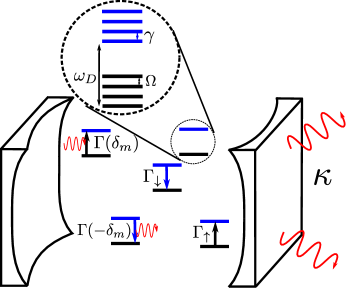
Figure 1: (Color online) Cartoon of the system showing the decay processes included in Eq. (6). The zoomed in view shows the energy level structure of the dye molecules.

II.1 Eliminating vibrational modes

If the coupling to rovibrational modes, $S$, is reasonably strong, then multiphonon effects will be important in describing the thermalization processes. To capture these effects it is convenient to make a polaron transformation $\hat{H}\to\hat{U}^{\dagger}\hat{H}\hat{U}$, where

$$\hat{U}=\exp\left[\sum_{i}\sqrt{S}\hat{\sigma}_{i}^{z}(\hat{b}_{i}-\hat{b}^{\dagger}_{i})\right].$$ (2)

This results in a Hamiltonian of the form (ignoring unimportant constants),

$$H=\sum_{m}\omega_{m}\hat{a}^{\dagger}_{m}\hat{a}_{m}+\sum_{i}\frac{\omega_{D}}{2}\hat{\sigma}_{i}^{z}+\Omega\hat{b}^{\dagger}_{i}\hat{b}_{i}\\ +{g}\left(\hat{a}\hat{\sigma}_{i}^{+}\hat{D}_{i}+\hat{a}^{\dagger}\hat{\sigma}_{i}^{-}\hat{D}_{i}^{\dagger}\right),$$ (3)

where the displacement operator at site $i$ is $\hat{D}_{i}=\exp[2\sqrt{S}(\hat{b}^{\dagger}_{i}-\hat{b}_{i})]$. Since the coupling of molecules to the optical modes is weak, we then treat the dynamics perturbatively in $g$ while keeping all orders of $S$. To do this we write the Liouville equation for the reduced density operator treating the on site vibrational mode as a bath. Making the standard Born-Markov approximations as well as secularizing the resulting equation by removing any terms which oscillate quickly in the interaction picture one then arrives at the master equation Marthaler et al. (2011),

$$\dot{\hat{\rho}}=-i[\hat{H}_{0},\hat{\rho}]-\sum_{i,m}\left\{\frac{\kappa}{2}\mathcal{L}[\hat{a}_{m}]+\frac{\Gamma_{\uparrow}}{2}\mathcal{L}[\hat{\sigma}_{i}^{+}]+\frac{\Gamma_{\downarrow}}{2}\mathcal{L}[\hat{\sigma}_{i}^{-}]\right\}\hat{\rho}\\ +K(-\delta_{m})\left[\hat{a}_{m}\hat{\sigma}^{+}_{i},\hat{a}^{\dagger}_{m}\hat{\sigma}^{-}_{i}\hat{\rho}\right]+K^{\ast}(-\delta_{m})\left[\hat{\rho}\hat{a}_{m}\hat{\sigma}^{+}_{i},\hat{a}^{\dagger}_{m}\hat{\sigma}^{-}_{i}\right]\\ +K(\delta_{m})\left[\hat{a}^{\dagger}_{m}\hat{\sigma}^{-}_{i},\hat{a}_{m}\hat{\sigma}^{+}_{i}\hat{\rho}\right]+K^{\ast}(\delta_{m})\left[\hat{\rho}\hat{a}^{\dagger}_{m}\hat{\sigma}^{-}_{i},\hat{a}_{m}\hat{\sigma}^{+}_{i}\right].$$ (4)

The function $K(\delta)$ will be defined below, and $\delta_{m}$ represents the detuning between a given cavity mode and the bare dye frequency, $\delta_{m}=\omega_{m}-\omega_{D}$. In writing Eq. (4) we have also included additional Markovian loss terms which describe leakage from the cavity at rate $\kappa$ (assumed to be identical for all photon modes), incoherent pumping of molecules to the excited electronic state at rate $\Gamma_{\uparrow}$ and incoherent decay to the ground state at rate $\Gamma_{\downarrow}$ which describes fluorescence processes which emit photons into non-cavity modes. These are described by the usual Lindblad superoperator defined as $\mathcal{L}[\hat{X}]\hat{\rho}=\{\hat{X}^{\dagger}\hat{X},\hat{\rho}\}-2\hat{X}\hat{\rho}\hat{X}^{\dagger}$.

The function $K(\delta)$ which appears in the vibration induced terms is given by the Fourier transform of the retarded correlation function of displacement operators, broadened by (convolved with) the incoherent pumping and decay of the electronic degrees of freedom Marthaler et al. (2011):

$$K(\delta)=g^{2}\int_{0}^{\infty}dt\langle{\hat{D}^{\dagger}_{i}(t)\hat{D}_{i}(0)}\rangle{\rm e}^{-(\Gamma_{\uparrow}+\Gamma_{\downarrow})|t|/2}{\rm e}^{-i\delta t}.$$ (5)

Here $\hat{D}_{i}(t)$ is the displacement operator in the interaction picture. The real parts of this function can be collected into Lindblad terms which give rise to decay processes which simultaneously (de)excite a molecule and (emit) absorb a photon. These processes, along with the other gain and loss terms, are shown schematically in Fig. 1. The imaginary parts (Lamb shifts) on the other hand can be absorbed into the Hamiltonian evolution to give the master equation,

$$\dot{\hat{\rho}}=-i[\tilde{\hat{H}}_{0},\hat{\rho}]-\sum_{i,m}\left\{\frac{\kappa}{2}\mathcal{L}[\hat{a}_{m}]+\frac{\Gamma_{\uparrow}}{2}\mathcal{L}[\hat{\sigma}_{i}^{+}]+\frac{\Gamma_{\downarrow}}{2}\mathcal{L}[\hat{\sigma}_{i}^{-}]\right.\\ \left.+\frac{\Gamma(-\delta_{m})}{2}\mathcal{L}[\hat{a}^{\dagger}_{m}\hat{\sigma}^{-}_{i}]+\frac{\Gamma(\delta_{m})}{2}\mathcal{L}[\hat{a}_{m}\hat{\sigma}^{+}_{i}]\right\}\hat{\rho}.$$ (6)

The rate $\Gamma(\delta)$ arises from the real part of the correlation function of displacement operators $\Gamma(\delta)=2{\rm Re}[K(\delta)]$. The Hamiltonian in this equation has been renormalized by the interaction with the bath provided by the vibrational degrees of freedom

$$\tilde{\hat{H}}_{0}=\sum_{m,i}\tilde{\delta}_{m}\hat{a}^{\dagger}_{m}\hat{a}_{m}+\eta_{m}\hat{a}^{\dagger}_{m}\hat{a}_{m}\hat{\sigma}_{i}^{+}\hat{\sigma}_{i}^{-}.$$ (7)

In this expression we have shifted into a frame rotating at the frequency of the bare molecular transition so that only the detunings $\delta_{m}$, and not the individual values of $\omega_{m}$, $\omega_{D}$ appear. The energy shifts in the Hamiltonian above are given by $\eta_{m}={\rm Im}[K(-\delta_{m})-K(\delta_{m})]$ and $\tilde{\delta}_{m}=\delta_{m}+{\rm Im}[K(\delta_{m})]$. Since, in the photon number basis, Eq. (7) is diagonal (it only couples populations to other populations), these Lamb shifts do not affect the dynamics at order $g^{2}$. As our approximation is based on expanding in powers of the small parameter $g/\omega_{0}$, these Lamb shifts can therefore be ignored, at least below or at threshold.

The displacement operator correlation function which is required to find the decay rates in the master equation can be calculated exactly by considering the Schwinger-Keldysh path integral:

$$\langle{\hat{D}^{\dagger}_{i}(t)\hat{D}_{i}(0)}\rangle=\int\mathcal{D}(b\bar{b}){\rm e}^{i\tilde{S}}D^{\ast}_{i}(t)D_{i}(0),$$ (8)

where the action, $\tilde{S}$, is given by

$$\tilde{S}=\int\frac{d\nu}{2\pi}\;{\boldsymbol{\bar{b}}}\,G^{-1}\,{\boldsymbol{b}}.$$ (9)

This is written in terms of the inverse Green’s function, $G^{-1}$, for an harmonic oscillator coupled to a thermal bath. Writing the fields in the Keldysh rotated basis, ${\boldsymbol{b}}=(b_{cl},b_{q})^{T}$, the inverse Green’s function takes the form Kamanev (2011):

$$G^{-1}=\begin{pmatrix}0&\nu-\Omega-\frac{i\gamma}{2}\\ \nu-\Omega+\frac{i\gamma}{2}&i\gamma\coth\left(\frac{\beta\nu}{2}\right)\end{pmatrix},$$ (10)

where $\beta=1/k_{B}T$ is the inverse temperature. To proceed we write the correlation function in the form:

$$\langle{\hat{D}^{\dagger}_{i}(t)\hat{D}_{i}(0)}\rangle=\int\mathcal{D}(b_{i},\bar{b}_{i}){\rm e}^{i\tilde{S}+Q},$$ (11)

where $Q$ corresponds to the sum of the exponents from $D_{i}^{\ast}(t)$ and $D_{i}(0)$. After completing the square and carrying out the Gaussian integral this gives

$$\langle{\hat{D}^{\dagger}_{i}(t)\hat{D}_{i}(0)}\rangle=\\ \exp\left[-i\int\frac{d\nu}{2\pi}|q(\nu)|^{2}\left(G^{A}+G^{R}+G^{K}\right)\right],$$ (12)

where $q(\nu)=\sqrt{2S}[\exp(i\nu t)-1]$ and $G^{A/R/K}$ are the advanced, retarded and Keldysh Green’s functions respectively. From the inverse of Eq. (10) we find that the correlation function is Wilson-Rae and Imamoğlu (2002); McCutcheon and Nazir (2011); Marthaler et al. (2011)

$$\langle{\hat{D}^{\dagger}_{i}(t)\hat{D}_{i}(0)}\rangle=\\ \exp\left[-\frac{2S\gamma}{\pi}\int_{-\infty}^{\infty}d\nu\frac{2\sin^{2}\left(\frac{\nu t}{2}\right)\coth\left(\frac{\beta\nu}{2}\right)+i\sin\left(\nu t\right)}{(\Omega-\nu)^{2}+\frac{\gamma^{2}}{4}}\right].$$ (13)

From this expression we can then evaluate the Fourier transform in Eq. (5), and thus find the rates $\Gamma(\pm\delta_{m})$ determining emission and absorption into various photon modes, as well as the corresponding Lamb shifts. The appearance of a thermal photon distribution can be traced back to properties of these rates, and thus of the correlator given in Eq. (13). Specifically, thermalization requires that the correlation function obeys the Kubo-Martin-Schwinger relation Kubo (1957); *Martin1959, $\langle{\hat{D}^{\dagger}_{i}(t)\hat{D}_{i}(0)}\rangle=\langle{\hat{D}_{i}^{\dagger}(-t-i\beta)\hat{D}_{i}(0)}\rangle$. If $\Gamma_{\uparrow},\Gamma_{\downarrow}$ could be neglected, substituting this into Eq. (5) would lead directly to the Kennard-Stepanov relation Kennard (1918); *Kennard1926; *Stepanov1957 between emission and absorption rates, $\Gamma(\delta)={\rm e}^{\beta\delta}\Gamma(-\delta)$. However, the expression in Eq. (5) involves the convolution of this spectrum with a Lorentzian due to the pump and decay, and so the Kennard-Stepanov relation only holds at small detunings. As the detuning is increased $\Gamma(\delta)$ ceases to obey this relation because the tails of $\Gamma(\delta)$ arise from the Lorentzian broadening with width $\Gamma_{\uparrow}+\Gamma_{\downarrow}$. The noise temperature of this pump term is not in thermal equilibrium with the dye. We therefore model this pump by a white noise (i.e. infinite temperature) bath Lax (2000). For experimentally realistic parameter values these effects do not cause any significant deviation from the Kennard-Stepanov relation.

At this point we note that had we instead used the quantum regression theorem to evaluate the correlator $\langle{\hat{D}^{\dagger}_{i}(t)\hat{D}_{i}(0)}\rangle$, the resulting expression would not have obeyed the Kennard-Stepanov relation. The quantum regression theorem is known to be incapable of describing finite temperature fluctuation dissipation relations Ford and O’Connell (1996); Lax (2000). The results of the quantum regression calculation would correspond to replacing $\nu\to\Omega$ in the Keldysh component of the Green’s function in Eq. (10) i.e. assuming that the bath occupation can be represented by sampling it at a single frequency $\nu=\Omega$.

As discussed previously in our Letter, it is the existence of the Kennard-Stepanov relation that causes the thermal state of the rovibrational degrees of freedom to be imprinted on the photon distribution. The thermal spectrum comes about not because the emission is thermal, but because the ratio of emission to absorption is thermally weighted. As noted above, this breaks down in the tails of the molecular spectrum. Note that in what follows, we consider cases where the lowest cavity mode is detuned below the peak of the molecular spectrum, so that it is typically the lowest energy photon modes that fall in the tail of the spectrum, while the “thermal tail” of the photon distribution is near the center of the molecular spectrum. In addition to relying on the thermal nature of the spectrum, such a mechanism of thermalization relies on the possibility of light being re-absorbed by the dye molecules before it escapes from the cavity. This also breaks down in the tails of the spectrum, where the absorption and emission rates become small. As we will discuss below, these points can be clearly seen in the time evolution towards a thermal distribution, and in the ways that the thermal distribution breaks down.

The quantum model we consider is thus fully defined by Eq. (4) along with the definitions of the rates via Eqs. (5) and (13). We summarize the parameters appearing in the model, and the values used in this manuscript, in table 1.

Parameter	Meaning	Value(s) used
$\delta_{0}$	Lowest cavity mode detuning	$-300$THz to $-100$THz
$\epsilon$	Cavity mode spacing	$5$THz
$\kappa$	Cavity mode decay rate	$100$MHz – $1$THz
$g$	Light-matter coupling strength	$1$GHz
$\Gamma_{\downarrow}$	Decay rate of excited electronic state	$1$GHz
$\Gamma_{\uparrow}$	Pumping rate of electronic states	Variable
$N$	Number of molecules	$10^{9}$
$\Omega_{j}$	Frequency of $j$th rovibrational mode	$5$THz - $60$THz
$\gamma_{j}$	Relaxation (thermalization) rate of mode $j$	$5$THz - $50$THz
$S_{j}$	Huang-Rhys factor of mode $j$	$0.5$
$\Gamma(-\delta_{m})$	Emission rate into cavity mode $m$
$\Gamma(\delta_{m})$	Absorption rate from cavity mode $m$
${\Gamma}_{\uparrow}^{\rm tot},{\Gamma}_{\downarrow}^{\rm tot}$	Electronic transition rates including contribution of cavity modes

Table 1: Summary of bare and derived parameters for the quantum model we consider. For each parameter, the values or range of values used in this manuscript are quoted, as appropriate.

II.2 Multiple vibrational modes

The absorption and emission spectra of dye molecules observed in experiments Schäfer (1990); Klaers et al. (2010a) show a structure with multiple peaks. There are two possible origins of this feature; either the relaxation time of the rovibrational states is long enough to allow multi-phonon effects to be spectrally resolved, or there are multiple vibrational modes with different frequencies which are important. The very rapid thermalization of the system seen in experiments Klaers et al. (2010a) rules out the first of these options and so here we consider the second case. To do this we modify the Hamiltonian in Eq. (1) to include multiple vibrational modes for each molecule, so that it now reads

$$\hat{H}=\sum_{m}\omega_{m}\hat{a}^{\dagger}_{m}\hat{a}_{m}+g\sum_{m,i}\left(\hat{a}_{m}\hat{\sigma}_{i}^{+}+\hat{a}^{\dagger}_{m}\hat{\sigma}_{i}^{-}\right)\\ +\sum_{i}\frac{\omega_{D}}{2}\hat{\sigma}_{i}^{z}+\sum_{j}\Omega_{j}\left[\hat{b}^{\dagger}_{i,j}\hat{b}_{i,j}+\sqrt{S_{j}}\hat{\sigma}_{i}^{z}(\hat{b}_{i,j}+\hat{b}^{\dagger}_{i,j})\right].$$ (14)

There is now a sum over $j$ which indexes the rovibrational modes at each site and so $\hat{b}^{\dagger}_{i,j}$ is an operator which creates a vibrational excitation in mode $j$ of molecule $i$. We can then go through exactly the same calculation as in the previous section. This results in a master equation with exactly the same form as Eq. (6) but where the displacement operator is now a product of single mode operators and hence the correlation function now includes contributions from all of the vibrational modes

$$\langle{\hat{D}^{\dagger}_{i}(t)\hat{D}_{i}(0)}\rangle=\exp\left(-\sum_{j}\frac{2S_{j}\gamma_{j}}{\pi}f_{j}(t)\right),$$

$$f_{j}(t)=\int_{-\infty}^{\infty}d\nu\frac{2\sin^{2}\left(\frac{\nu t}{2}\right)\coth\left(\frac{\beta\nu}{2}\right)+i\sin\left(\nu t\right)}{(\Omega_{j}-\nu)^{2}+\frac{\gamma_{j}^{2}}{4}}.$$ (15)

We note that the spectrum which results from this expression still obeys the Kennard-Stepanov relation with the same caveats as above.

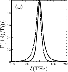
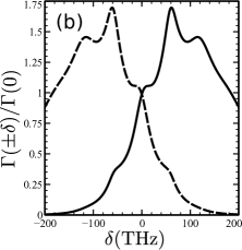
Figure 2: The effective absorption (solid) and emission (dashed) rates, $\Gamma(\pm\delta)$ for different vibrational mode structures. In (a) we show the case of one mode with parameters $S=0.5$, $\Omega=5$THz, $\gamma=50$THz. In (b) we also include a second mode with $S=0.5$, $\Omega=60$THz, $\gamma=30$THz

We show examples of the resulting absorption and emission spectra including one and two vibrational modes in Fig. 2. In the case with only one low frequency mode included the spectrum simply consists of a single peak broadened by the thermalization rate. The difference between the location of the maxima in the absorption and emission scales with the coupling between the vibrational and electronic degrees of freedom, $S$. When we add an extra higher frequency mode we see that the spectrum gains multiple peaks at integer multiples of the second mode frequency and reduces the relative weight of the spectrum around $\delta=0$ (the zero phonon line). This type of spectrum is much closer to that seen in the absorption and emission of the dyes used in the photon condensation experiments Klaers et al. (2010a).

Using this multi-peaked type of spectrum, however, does not affect the physics which we will go on to discuss. The mechanisms of thermalization and the way they break down do not depend on the details of the absorption and emission rates. However, the behavior once thermalization has broken down will depend on the shape of the emission spectrum. For the remainder of this paper we use the simpler single mode case except where otherwise noted.

III Rate equation approximation

Having derived a full quantum model in the previous section, we next turn to study the properties of this model using a rate equation approximation. Such an approximation is valid when there are many molecules coupled to each photon mode, so that quantum correlations are suppressed by $1/N$. However, such an approximation is restricted to describing physics that depends only on the populations of the modes, and not on the off-diagonal coherences, or higher order statistics (such as $g^{(2)}$). As discussed below, a closed set of equations for the mode populations exists and this is considerably easier to solve than Eq. (6). We will however return in Section IV to discuss features beyond the scope of the rate equation.

III.1 Derivation of rate equation

To obtain the rate equation we write down an equation for the expectation value of the number of photons in a given mode $n_{m}=\langle{\hat{a}^{\dagger}_{m}\hat{a}_{m}}\rangle$ and make the semiclassical approximation that the density operator for the photons and molecules factorizes e.g. $\langle{\hat{a}^{\dagger}_{m}\hat{a}_{m}\hat{\sigma}^{+}}\rangle=\langle{\hat{a}^{\dagger}_{m}\hat{a}_{m}}\rangle\langle{\hat{\sigma}^{+}}\rangle$. This then leads to the set of coupled equations for the evolution of the populations of the photon modes, $n_{m}$, and for the probability of finding a molecule in its excited state, $p_{e}$. For $N$ dye molecules these are given by,

$$\begin{split}\frac{\partial{n_{m}}}{\partial{t}}=-\kappa n_{m}+N\left[\Gamma(-\delta_{m})(n_{m}+1)p_{e}\right.\\ \left.-\Gamma(\delta_{m})n_{m}(1-p_{e})\right],\end{split}$$ (16)

$$\frac{\partial{p_{e}}}{\partial{t}}=-{\Gamma}_{\downarrow}^{\rm tot}(n_{m})p_{e}+{\Gamma}_{\uparrow}^{\rm tot}(n_{m})(1-p_{e}),$$ (17)

where we have defined the rates:

$${\Gamma}_{\uparrow}^{\rm tot}(n_{m})=\Gamma_{\uparrow}+\sum_{m}g_{m}\Gamma(\delta_{m})n_{m},$$ (18)

$${\Gamma}_{\downarrow}^{\rm tot}(n_{m})=\Gamma_{\downarrow}+\sum_{m}g_{m}\Gamma(-\delta_{m})(n_{m}+1).$$ (19)

We see from the expressions above, that the rate of emission and absorption into a given cavity mode depend on the number of excited state molecules, and on the number of photons already in that mode, exactly as one would expect. Similarly, the transition rates between the electronic states depend on the numbers of photons in all modes. As we will see below, this has the consequence that the populations of the modes are coupled, and leads to the emergence of a chemical potential for photons.

III.1.1 Steady state distribution

If we are only interested in the steady state properties of the photon distribution, then we may adiabatically eliminate the molecular degrees of freedom and obtain the self-consistent expression for the photon distribution

$$\kappa n_{m}=N\frac{\Gamma(-\delta_{m})(n_{m}+1){\Gamma}_{\uparrow}^{\rm tot}-\Gamma(\delta_{m})n_{m}{\Gamma}_{\downarrow}^{\rm tot}}{{\Gamma}_{\uparrow}^{\rm tot}+{\Gamma}_{\downarrow}^{\rm tot}}.$$ (20)

In the equilibrium limit when the losses from the cavity are negligible, $\kappa,\Gamma_{\downarrow},\Gamma_{\uparrow}\to 0$, this expression results in a Bose-Einstein distribution for the photons which satisfies

$$\frac{n_{m}+1}{n_{m}}=e^{\beta\delta_{m}}\frac{{\Gamma}_{\downarrow}^{\rm tot}}{{\Gamma}_{\uparrow}^{\rm tot}}.$$ (21)

We are thus able to define an effective chemical potential $\mu=k_{B}T\ln{{\Gamma}_{\uparrow}^{\rm tot}/{\Gamma}_{\downarrow}^{\rm tot}}$ which, far below threshold, when the populations of all the photon modes are negligible, can be approximated as $\mu_{0}=k_{B}T\ln{{\Gamma}_{\uparrow}^{\rm tot}(0)/{\Gamma}_{\downarrow}^{\rm tot}(0)}$. NB, while the effective pumping rate for an empty cavity ${\Gamma}_{\uparrow}^{\rm tot}(0)=\Gamma_{\uparrow}$, the effective decay rate ${\Gamma}_{\downarrow}^{\rm tot}(0)\neq\Gamma_{\downarrow}$, due to existence of spontaneous emission into the cavity modes.

In Fig. 3 we show the behavior of the system as we increase the pump strength through this threshold. We see that the total number of photons in the cavity $N_{\rm phot}=\sum_{m}g_{m}n_{m}$ has a sharp transition at the same point as the number of excited molecules saturates. This also corresponds to the chemical potential reaching the energy of the ground mode of the cavity. We note that the behavior of both $N_{\rm phot}$ and $p_{e}$ is qualitatively what is expected for the transition to a lasing state, but the saturated value for $p_{e}$ is much lower than the electronic inversion point. Also note that in a laser it is impossible to identify a chemical potential. In Fig. 3(c) the chemical potential defined in this way shows exactly the same behavior as is typically associated with a BEC transition. Below threshold we see that the chemical potential matches very well to the simple expression derived above assuming the cavity is empty; at and above threshold, the chemical potential locks to $\mu=\delta_{0}$.

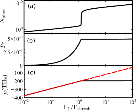
Figure 3: (Color online) Steady state behavior of our model as it is pumped through the BEC transition. (a) shows the total number of photons in the cavity. (b) gives the fraction of molecules in the excited state and (c) shows the effective chemical potential. In (c) we also plot (as the red, dashed curve) the simple below threshold expression $\mu_{0}=k_{B}T\ln{{\Gamma}_{\uparrow}^{\rm tot}(0)/{\Gamma}_{\downarrow}^{\rm tot}(0)}$. The parameters used are $S=0.5$, $\gamma=50$THz, $\Omega=5$THz, $\kappa=100$MHz, $T=300$K, $N=10^{9}$, $g=1$GHz, $\delta_{0}=-200$THz, $\Gamma_{\downarrow}=1$GHz.

III.1.2 Threshold condition

Before discussing the phase boundary of the photon condensate state, we must first define the threshold condition carefully. Care is required because we consider a finite system in an harmonic trap, and so the boundary is not sharp. We wish to define a threshold condition in terms of the number of photons in the ground mode of the cavity, $n_{0}$. A naive approach would be to define the threshold when this reaches a fixed value, e.g. $1$, however if applied to the equilibrium limit, this gives a complicated formula for the critical temperature. In equilibrium, the appropriately defined thermodynamic limit Bagnato and Kleppner (1991) has a critical temperature $k_{B}T=\epsilon\sqrt{6N_{\text{phot}}}/\pi$, where $N_{\text{phot}}$ is the total number of photons in the cavity. We aim to define the threshold condition consistently with this.

We begin by assuming the system is in thermal equilibrium. For our 2D harmonically trapped gas, the energy of the mode with $n$ and $m$ photons in the two directions and mode spacing $\epsilon$ is given by $\delta_{0}+(n+m)\epsilon$. The total number of particles in the Bose-Einstein distribution is therefore

$$N_{\rm phot}=\sum_{n,m}\left[{\rm e}^{\beta[(n+m)\epsilon-\mu+\delta_{0}]}-1\right]^{-1}$$

$$=\sum_{j=1}^{\infty}\left(1-{\rm e}^{-\beta\epsilon j}\right)^{-2}{\rm e}^{\beta(\mu-\delta_{0})j}.$$ (22)

In the thermodynamic limit, $\epsilon\to 0$, the transition occurs exactly at $\mu=\delta_{0}$, and so ${\rm e}^{\beta(\mu-\delta_{0})}=1$. To leading order in $\beta\epsilon$ this gives the critical photon number:

$$N_{\rm phot}=\frac{(k_{B}T)^{2}}{\epsilon^{2}}\sum_{j=1}^{\infty}\frac{1}{j^{2}}=\frac{(k_{B}T)^{2}\pi^{2}}{6\epsilon^{2}},$$ (23)

which diverges as $\epsilon\to 0$. Even at non-vanishing $\epsilon$, if we were to define the threshold condition as $\mu=\delta_{0}$, we would find a ground mode population $n_{0}\rightarrow\infty$. As such, we cannot use $\mu=\delta_{0}$ as the threshold condition. To regularize this we calculate the next-to-leading order contribution to the total particle number in $\beta\epsilon$. This is given by

$$N_{\rm phot}\simeq\frac{1}{(\beta\epsilon)^{2}}\sum_{j=1}^{\infty}\frac{{\rm e}^{\beta(\mu-\delta_{0})j}}{j^{2}\left(1-\beta\epsilon\right)^{j}},$$ (24)

where we have used $1-j\beta\epsilon=(1-\beta\epsilon)^{j}$ to order $\beta\epsilon$. If we define the threshold as occurring when $N_{\text{phot}}$ reaches the value given in Eq. (23), then we must choose Bagnato and Kleppner (1991); Hadzibabic et al. (2008); Kirton and Keeling (2013)

$$e^{\beta(\mu-\delta_{0})}=1-\beta\epsilon\qquad\to\qquad{n_{0}}=\frac{1}{\beta\epsilon}-1.$$ (25)

To leading order in $\epsilon$, we thus use $n_{0}=1/\beta\epsilon$ to define the threshold condition. From this we can go on to define a threshold pump power, $\Gamma_{\rm thresh}$ as the value of $\Gamma_{\uparrow}$ required for this population to be reached. Note that since $N_{\text{phot}}\sim 1/(\beta\epsilon)^{2}$, the criterion we use corresponds to $n_{0}\sim\sqrt{N_{phot}}$, and so can be understood as distinguishing macroscopic ($n_{0}\sim N_{\text{phot}}$) and microscopic ($n_{0}\sim 1$) occupations of a single mode.

Away from thermal equilibrium, when the system does not obey a Bose-Einstein distribution, it will still be useful to define the same threshold but in this case we will use the slightly more general definition $\max\{n_{m}\}=1/\beta\epsilon$. That is, whenever one mode of the cavity exceeds the required population.

III.2 Breakdown of thermalization

We have shown that, for weak enough losses, the master equation given in Eq. (6), has as its steady state solution an equilibrium Bose-Einstein distribution. As such, the steady state of this equation shows a condensation transition at a critical photon density, or equivalently a critical pump power. To reach this thermal equilibrium state we have shown that it is necessary for the dye molecules to thermalize with the photon distribution. Hence, the timescale over which the thermalization happens must be shorter than the lifetime of photons inside the cavity. In our earlier Letter Kirton and Keeling (2013) we showed how the distribution crosses over to that of a standard laser as the cavity lifetime is decreased. In this manuscript we instead concentrate on varying other properties of the cavity, and the vibrational properties of the dye molecules.

III.2.1 Changing the cavity cutoff

We begin by considering what happens when the length of the cavity is changed, as was experimentally Klaers et al. (2010a) tested. When the length of the cavity is increased the energy of the lowest frequency mode it can support decreases. The detuning of these low energy modes from the dye molecule resonance then increases, and so the modes have very small absorption and emission rates $\Gamma(\pm\delta_{0})$. Thus, for these modes, cavity losses compete with absorption and emission.

We show the effects of decreasing $\delta_{0}$ on the system in Fig. 4(a) by comparing the numerical steady state distributions (solid lines) to Bose-Einstein distribution fits to the tail of the numerics (dashed lines). In order to perform this fit we first fix the temperature to be that of the dye, and then use the chemical potential as a variable parameter to fit to the thermal tail of the numerical results. As can be seen, for the parameters used in Fig. 4(a) a thermal tail with the correct temperature is always present (since this thermal tail is near the center of the molecular spectrum, $\delta=0$, thermalization is good). Adjusting the chemical potential corresponds to fitting an overall scale for the intensity of the thermal tail, thus this can be fit by matching a single point in the tail of the distribution. Since such a fit is matched only to the higher energy photon modes, there is no guarantee as to how the extracted chemical potential $\mu$ compares to the lowest energy photon mode energy $\delta_{0}$. In equilibrium, $\mu\leq\delta_{0}$ with equality holding above threshold, when the chemical potential locks to the bottom of the spectrum. Since $\mu$ is extracted from the high energy tail, whether or not it matches the low energy peak and thus locks at the cutoff frequency $\delta_{0}$ can provide a good measure of the degree of thermalization of the distribution, as discussed further below.

When the cutoff is $-100$THz (the red curve) we see that the system reaches thermal equilibrium and the photon populations are well described by a Bose-Einstein distribution. Reducing $\delta_{0}$ to $-200$THz (the blue curve) we see that the match to a Bose-Einstein distribution is still good but there is a slight discrepancy in the prediction of the location of the peak calculated just from looking at the thermal tail. This disagreement between the numerical results and an equilibrium distribution is even more apparent in the curve with a detuning of $-300$THz (the green curve) where the lowest energy modes are completely out of equilibrium and the macroscopically occupied mode is one of the excited modes of the cavity. As discussed above, this breakdown is due to the cavity losses being too fast for these modes with low absorption and emission rates to thermalize. This is the same mechanism as discussed in our previous work Kirton and Keeling (2013), where we considered the effect of reducing the cavity lifetime. We note that the reason that the thermal tails of the photon distributions are not exactly parallel is that these curves are Bose-Einstein distributions multiplied by a degeneracy factor which results in logarithmic corrections to the tail. These become more important for smaller cutoff energies.

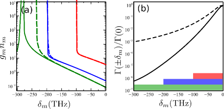
Figure 4: (Color online) (a) Photon distribution just above threshold pump power, illustrating the effect of decreasing the energy of the lowest cavity mode, $\delta_{0}$. The green curve is $\delta_{0}=-300$THz, blue is $\delta_{0}=-200$THz, and red is $\delta_{0}=-100$THz. The dashed lines show Bose-Einstein fits to the tails of the data. (b) The absorption (solid) and emission (dashed) rates for the same parameters. The shaded regions show which modes are included for the same colored curves as in (a). All parameters except $\delta_{0}$ are the same as in Fig. 3.

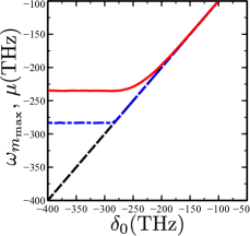
Figure 5: (Color online) Comparison between fitted chemical potential, energy of maximally populated mode and cavity cutoff, as the cutoff is varied. Above threshold in equilibrium, the maximally occupied mode and effective chemical potential both lock to the cavity cutoff (dashed line). The solid (red) and dot-dash (blue) lines correspond, respectively, to the fitted chemical potential, and energy of the maximally populated mode as extracted from the steady state distribution for the same parameters as given in Fig. 3.

In equilibrium, above threshold, both the maximum in the photon distribution, $\omega_{m_{\rm max}}$, and the value of the chemical potential, $\mu$ (found from the Bose-Einstein fit to the tail) lock at the energy of the ground mode of the cavity, $\delta_{0}$. As such, the difference between these quantities and the ground mode energy can be used to demonstrate the breakdown of thermalization. In Fig. 5 we show the way in which these three quantities vary as we change the cavity cutoff energy. At small values of $\delta_{0}$ these all match the equilibrium expectation (the energy of the cavity ground mode). As the detuning is increased the first change is that the fitted chemical potential starts to deviate, while the macroscopically occupied mode of the cavity remains the cavity ground mode. This situation corresponds to that seen in the blue curve of Fig. 4(a), where a slight deviation from a thermal distribution is visible. As the detuning is increased even further, the ground mode of the cavity becomes far detuned from the molecular emission peak, and so the rates of absorption and emission can no longer compete with cavity losses. One then has that an excited mode of the cavity gains a macroscopic occupation and so the energy of this maximally populated mode deviates from the equilibrium prediction. It is notable that at the smallest values of $\delta_{0}$, both the fitted chemical potential and the energy of the maximally populated modes saturate. This occurs because the additional low energy cavity modes have negligible population (as cavity loss beats emission rate), and so the behavior of the system is not affected by including these extra low energy modes.

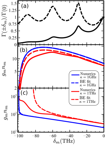
Figure 6: (Color online) The effect of a peaked absorption and emission spectrum. In (a) we show the form of $\Gamma(\pm\delta_{m})$ when we included a vibrational mode which is not overdamped (solid line shows absorption, dashed line emission). In (b) and (c) we show the effect of increasing the cavity losses for this spectrum below ($\Gamma_{\uparrow}=0.5\Gamma_{\rm thresh}$) and above ($\Gamma_{\uparrow}=2.5\Gamma_{\rm thresh}$) threshold respectively. In each case we plot the behavior for two cavity loss rates: $\kappa=1$THz (red) and $\kappa=1$GHz (blue). The dashed lines are the fit to a Bose-Einstein distribution. Other parameter values are the same as Fig. 3 except as follows: The two vibrational modes are characterized by $S_{1}=0.1$, $\Omega_{1}=5$THz, $\gamma_{1}=50$THz, $S_{2}=0.5$, $\Omega_{2}=30$THz, $\gamma_{2}=5$THz.

III.2.2 Changing the properties of the dye molecules

By changing the properties of the dye molecules it is possible to change the functional form of $\Gamma(\delta)$. In particular, by introducing coupling to extra vibrational modes, as discussed in Sec. II.2, it is possible to engineer a form for $\Gamma(\delta)$ which has multiple peaks. To achieve such a multi-peaked structure, one needs spectrally resolved vibrational sidebands, which requires that (some of) the vibrational modes must have frequencies larger than their linewidths, i.e. be underdamped. An example of this type of spectrum is shown in Fig. 6(a). This is similar to the type of spectrum seen experimentally Klaers et al. (2010a) but with a more exaggerated multi-peaked structure. We note that while the spectrum now looks very different to the one used in the rest of this paper it still obeys the Kennard-Stepanov relation and so in thermal equilibrium will give rise to a Bose-Einstein distribution for the photons. We see that this is the case in Fig. 6(b) and (c) where for small cavity losses (the blue solid curve) the numerical results match well with the Bose-Einstein fit both above and below threshold. As the losses from the cavity are increased we see that the distribution becomes non-thermal, but it does so in a more complicated way than when the absorption and emission spectra have only a single peak. In this case, the modes close to the minima in $\Gamma(\delta)$ are the ones which are no longer able to thermalize, since the absorption and emission rates here are small enough that the cavity lifetime is too short for thermal equilibrium to be reached. This causes the complex non-monotonic photon spectra seen in the solid red curves of Fig. 6 (b) and (c) which now significantly deviate from the equilibrium fit shown by the dashed curve.

The results above, which show how it is possible to break the thermalization process, give motivation to the choice of two possible criteria for thermalization which characterize the behavior of the system at or near threshold and determine whether it is in thermal equilibrium. Firstly, we can look at which mode of the cavity gains a macroscopic occupation, $\omega_{m_{\rm max}}$, when we pump the system above threshold. When this mode is the ground mode of the cavity the system is close to thermal equilibrium but when this mode is one of the excited cavity the distribution has failed to thermalize. Secondly, we can look at the chemical potential of a fit to the distribution at or above threshold. If this is close to the ground mode energy then the system is in thermal equilibrium. These allow us to draw “phase diagrams” which separate regions in which the system looks like a thermal equilibrium condensate from those where it is more like the non-thermal state of a laser. The algorithm for generating these plots is as follows: for each set of parameter values the pump power is increased until the threshold (as described in Sec. III.1.2) is reached, then the number of the mode with the largest population and the chemical potential of the fit to the tail of the thermal distribution are recorded.

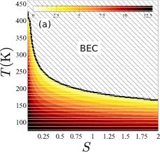
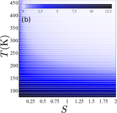
Figure 7: (Color online) Criteria for thermalization vs. $S$ and $T$. In (a) the color shows the index of the mode which gains a macroscopic occupation, the solid line separates the region where the ground mode condenses (hashed) from the region where excited cavity modes are macroscopically occupied. In (b) we show a similar diagram but with the ‘order parameter’ $\beta(\mu-\delta_{0})$.

We begin by examining how varying the strength of the coupling between electronic and vibrational states of the dye molecules, $S$, can affect the thermalization process. The Huang-Rhys parameter, $S$, describes the difference in displacement between the lowest energy vibrational state in the ground electronic manifold and the lowest energy state in the excited electronic manifold in units of the harmonic oscillator length. In Fig. 7, we look at the behavior of the two criteria described above in the $S$ vs. $T$ plane. For the chemical potential we plot the dimensionless quantity $\beta(\mu-\delta_{0})$ which is zero in thermal equilibrium and becomes more positive as the thermalization breaks down.

In the limit $S\to 0$ the absorption and emission spectra are exactly symmetric and therefore equal, and so thermalization is never possible. Thus, the lasing–condensation crossover as identified by both the criteria discussed above moves to infinite temperature. As $S$ is increased, the asymmetry in the rates increases, and so the minimum temperature at which thermalization occurs decreases. We see however that there is a region where the lowest mode is macroscopically occupied, but the chemical potential fit to the tail deviates from this lowest mode. This is the same behavior as was seen in Fig. 4(b): macroscopic occupation of the lowest mode is a weaker criterion. As the temperature or $S$ is decreased the value of $\beta(\mu-\delta_{0})$ increases. As the system is brought further from thermal equilibrium the chemical potential fit to the tail of the distribution moves closer to the gain maximum of the dye.

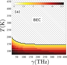
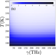
Figure 8: (Color online) Criteria for thermalization vs. $\gamma$ and $T$. Panel (a) shows the index of the mode which is macroscopically occupied above threshold. Panel (b) shows the chemical potential of the Bose-Einstein fit to the data, $\beta(\mu-\delta_{0})$.

We can also look at what happens when we vary the thermalization rate of the vibrational mode of the molecules, $\gamma$. The phase diagrams for these results in the $\gamma$ vs. $T$ plane are shown in Fig. 8. At small $\gamma$ the behavior is very similar to that seen at small values of $S$ above. This is to be anticipated, given the form of Eq. (13) where the combination $S\gamma$ appears as a prefactor in the exponent. Thus the $S\to 0$ and $\gamma\to 0$ limits are similar.

At large $\gamma$ a different behavior occurs due to the Lorentzian broadening of the vibrational resonances corresponding to the $\gamma^{2}$ term in the denominator. This broadening means the spectral weight, and thus both the absorption and emission rates, at any one frequency is suppressed. This has the consequence that cavity losses start to compete with absorption and emission, and thermalization breaks down. In contrast to the breakdown of thermalization at small $S$, small $\gamma$, or low temperature, the breakdown of thermalization at large $\gamma$ occurs simultaneously across the whole spectrum. i.e., rather than the just low energy modes becoming decoupled, all modes cease to follow a thermal distribution at once. Furthermore, because the breakdown of thermalization is not specific to the low energy modes, the macroscopically occupied mode remains the ground mode. This can be seen in Fig. 8 where with increasing $\gamma$ at large $\gamma$, the criterion for thermalization given by the fitted chemical potential moves to higher temperature, while the criterion given by which mode is occupied continues to move to lower temperatures.

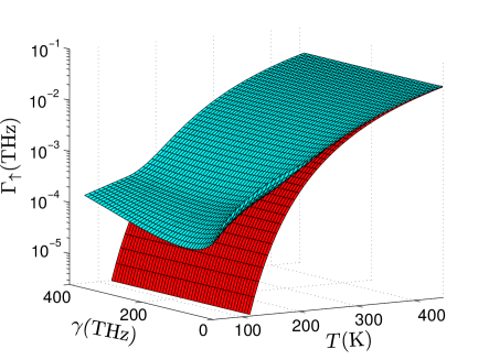
Figure 9: (Color online) Phase diagram for condensation/lasing, showing the required pump power for a mode to go above threshold (blue) compared to the equilibrium prediction (red).

A further way of quantifying the deviation from thermalization can be found be looking at the pumping strength required for the population in one of the modes to exceed the threshold population described in Sec. III.1.2. Comparing the value of $\Gamma_{\uparrow}$ necessary to exceed this threshold in $\max\{n_{m}\}$ to the predicted equilibrium value, $\Gamma_{\rm thresh}=\exp(\beta\delta_{0})\Gamma_{\downarrow}$, we see very similar behavior to the “phase diagram” for $\beta(\mu-\delta_{0})$. The actual threshold (blue) is always greater than the equilibrium prediction (red): the losses always need to be compensated. At low temperatures and small $\gamma$ we see the calculated threshold rise, this is as the lasing mode moves to higher excited states of the cavity as explained previously. We see that at large values of $\gamma$ there is also a rise in the threshold even in regions where the ground mode is maximally occupied; this is a signature of the thermalization process breaking down across the whole spectrum of the cavity.

III.3 Dynamics of thermalization

By integrating Eqs. (16)-(17) we can examine the time evolution of the system towards the steady state thermal equilibrium distribution. Examples of this are shown in Fig. 10, where we evolve the equations in time by turning on the pump at $t=0$. We may then follow the evolution from an initially empty cavity to the final Bose-Einstein distribution. In Fig. 10(a) and (c) we plot the photon distribution at various times as solid curves along with the equilibrium distribution as a dashed red curve. In Fig. 10(b) and (d) we plot the average energy of the photon distribution, $\langle{\delta_{m}}\rangle$ as a function of time. The markers on these curves indicate the times at which the traces in (a) and (c) were taken.

The first light emitted into the cavity modes follows closely the bare fluorescence spectrum, and so is dominated by photons with energies close to $\delta_{m}=0$. Thus, at these early times no thermalization is seen, and the same profile appears both above and below threshold. It is important to note that these early times are already longer than the timescale $1/\gamma$ required for the rovibrational states to reach thermal equilibrium. For the parameters used in Fig. 10 this rovibrational thermalization timescale is only $0.1$fs. The photons take longer to reflect this thermal distribution because thermalization of photons requires the balance of emission and absorption processes; i.e. it is only as photons are absorbed and re-emitted that a thermal distribution emerges from the balance between these processes. As this occurs, the mean of the distribution starts to shift towards the low energy modes of the cavity. Above threshold, as the equilibrium distribution is reached, the thermal tail slightly overshoots its steady state value and a large population appears in a mode slightly above $\delta_{0}$ before this finally moves to the ground mode. The thermalization time for each mode is set by $\Gamma(\delta_{m})$ and so is longer for the modes furthest away from the molecular transition frequency. The onset of a macroscopic occupation in the ground mode is accompanied by a kink in the mean photon frequency which occurs at the point where the macroscopic peak first appears. Finally, in both cases, the mean settles to its stationary value (very close to $\delta_{0}$ above threshold) as the steady state is reached. The themalization time which we find for these experimentally realistic parameters is of order 10-100ps, which is similar to the measured result Schmitt et al. (2014b).

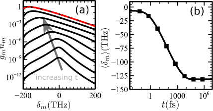
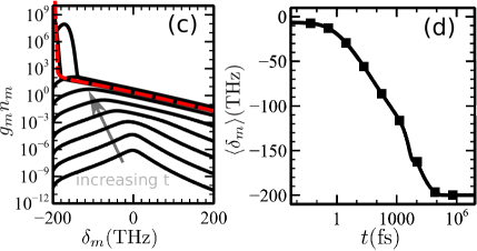
Figure 10: (Color online) Time evolution towards thermal equilibrium both below ($\Gamma_{\uparrow}=0.2\Gamma_{\rm thresh}$) (a)-(b) and above ($\Gamma_{\uparrow}=10\Gamma_{\rm thresh}$) (c)-(d) threshold. In (a) and (c) we show the photon distribution at different times, the dashed red curves show the steady state solution. In (b) and (d) we show the mean frequency of the photon intensity, $\langle{\delta_{m}}\rangle$, as a function of time. The squares show the locations at which the traces in (a) and (c) are taken. Parameters are the same as in Fig. 3.

IV Beyond the Rate Equation Model

To look at the correlations in the system it is necessary to go beyond the rate equation description above. The rate equations neglect the correlations between the light and dye beyond first order, and so are unable to capture the behavior of the variances and higher order moments of the distribution. In this section we will show how, using a master equation for the full probability distribution, one may calculate both the second order photon coherence, $g^{(2)}$, and the linewidth of the emission.

To simplify the calculation it is instructive to look at the single mode version of the model considered so far. To do this we ignore the modes which make up the thermal tail and concentrate only on the mode which condenses. In this case the master equation is given by

$$\dot{\hat{\rho}}=-i\delta[\hat{a}^{\dagger}\hat{a},\hat{\rho}]-\frac{\kappa}{2}\mathcal{L}[\hat{a}]\hat{\rho}-\sum_{i}\left\{\frac{\Gamma_{\uparrow}}{2}\mathcal{L}[\hat{\sigma}_{i}^{+}]+\frac{\Gamma_{\downarrow}}{2}\mathcal{L}[\hat{\sigma}_{i}^{-}]\right.\\ \left.+\frac{\Gamma(-\delta)}{2}\mathcal{L}[\hat{a}^{\dagger}\hat{\sigma}^{-}_{i}]+\frac{\Gamma(\delta)}{2}\mathcal{L}[\hat{a}\hat{\sigma}^{+}_{i}]\right\}\hat{\rho}.$$ (26)

To proceed we note that the steady state of the above equation can be written in the form $\hat{\rho}=\sum_{n,m}P_{n,m}\ket{n}\!\bra{n}\otimes\hat{\rho}_{m}$ where $\ket{n}$ is a photon number state and $\hat{\rho}_{m}=\sum_{\{s_{i}=0,1\}}\delta_{m,\sum_{i}\!s_{i}}\bigotimes_{i}|s_{i}\rangle\langle s_{i}|$ is the incoherent mixture of all molecular states with a total number of excited molecules $m$. This steady state is thus “diagonal” in the number space of photons and excited molecules, and the quantity $P_{n,m}$ gives the probability of finding $n$ photons and $m$ electronic excitations in the system. One can easily check that such an ansatz exactly satisfies Eq. (26) as long as $P_{n,m}$ obeys the equation:

$$\dot{P}_{n,m}=\kappa[(n+1)P_{n+1,m}-nP_{n,m}]\\ \begin{aligned} +&\Gamma_{\uparrow}[(N-m+1)P_{n,m-1}-(N-m)P_{n,m}]\\ +&\Gamma_{\downarrow}[(m+1)P_{n,m+1}-mP_{n,m}]\\ +&\Gamma(-\delta)[n(m+1)P_{n-1,m+1}-(n+1)mP_{n,m}]\end{aligned}\\ +\Gamma(\delta)[(n+1)(N-m+1)P_{n+1,m-1}-n(N-m)P_{n,m}].$$ (27)

Such a form is sufficient because the full quantum master equation in Eq. (6) is written within a secular approximation. This means that the evolution of diagonal and off-diagonal terms can be separated, as has been done here.

IV.1 Second order coherence $g^{(2)}$

We can the use this equation for $P_{n,m}$ to calculate the zero time delay second order quantum coherence of the emitted light field $g^{(2)}(0)$. This quantity is defined as

$$g^{(2)}(0)=1+\frac{\sigma_{n}^{2}-\langle{n}\rangle}{\langle{n}\rangle^{2}},$$ (28)

where we define averages and variances as $\langle{X}\rangle=\sum_{n,m}XP_{n,m}$ and $\sigma_{X}^{2}=\langle{(X-\langle{X}\rangle)^{2}}\rangle$ respectively. Such a correlation function has been experimentally measured Schmitt et al. (2014a) where it was found to smoothly cross over from thermal light with $g^{(2)}=2$ below threshold to coherent light with $g^{(2)}=1$ far above threshold. Below we show that such behavior is indeed reproduced by Eq. (27)

For small system sizes we can solve Eq. (27) numerically to find the steady state probability distribution. This then allows one to extract the required moments to find $g^{(2)}$. Unfortunately, direct numerical solution of Eq. (27) is only tractable for relatively small numbers of molecules $N$. The value of $N$ sets the variances of both $n$ and $m$, and so with increasing $N$, the number of non-zero values of $P_{n,m}$ grows. This means that brute force numerics is not feasible with realistic values of $N\simeq 10^{9}$. In this large system size limit we can however get a good approximation to the behavior of the system above threshold by writing expressions for the moments and truncating at second order. This is equivalent to assuming that the full probability distribution is Gaussian. Such an assumption is reasonable above threshold, but fails at low pump powers. For a Gaussian distribution, one need only calculate the first and second moments of the distribution, as all moments factorize. The equations of motion for the first moments, $\partial_{t}\langle n\rangle,\partial_{t}\langle m\rangle$ give:

$$0= -\kappa\langle{n}\rangle+\Gamma(-\delta)[(\langle{n}\rangle+1)\langle{m}\rangle+\sigma^{2}_{nm}]$$

$$-\Gamma(\delta)[\langle{n}\rangle(N-\langle{m}\rangle)-\sigma^{2}_{nm}],$$ (29)

$$0= \Gamma_{\uparrow}(N-\langle{m}\rangle)-\Gamma_{\downarrow}\langle{m}\rangle$$

$$-\Gamma(-\delta)[(\langle{n}\rangle+1)\langle{m}\rangle+\sigma^{2}_{nm}]$$

$$+\Gamma(\delta)[\langle{n}\rangle(N-\langle{m}\rangle)-\sigma^{2}_{nm}],$$ (30)

while the equations of motion for the second order moments give rise to the following conditions

$$\begin{split}0=-\kappa\left(-\langle{n}\rangle+2\sigma_{n}^{2}\right)+\Gamma(-\delta)\left[(\langle{n}\rangle+1)\langle{m}\rangle+2\sigma^{2}_{n}\langle{m}\rangle+\sigma^{2}_{nm}(2\langle{n}\rangle+3)\right]\\ -\Gamma(\delta)\left[-\langle{n}\rangle(N-\langle{m}\rangle)+2\sigma_{n}^{2}(N-\langle{m}\rangle)-\sigma^{2}_{nm}(2\langle{n}\rangle-1)\right],\end{split}$$ (31)

$$\begin{split}0=\Gamma_{\uparrow}\left[(N-\langle{m}\rangle)-2\sigma_{m}^{2}\right]-\Gamma_{\downarrow}\left[-\langle{m}\rangle+2\sigma_{m}^{2}\right]-\Gamma(-\delta)\left[-(\langle{n}\rangle+1)\langle{m}\rangle+2\sigma_{m}^{2}(\langle{n}\rangle+1)+\sigma^{2}_{nm}(2\langle{m}\rangle-1)\right]\\ +\Gamma(\delta)\left[\langle{n}\rangle(N-\langle{m}\rangle)-2\sigma^{2}_{m}\langle{n}\rangle+\sigma^{2}_{nm}(-2\langle{m}\rangle+2N-1)\right],\end{split}$$ (32)

$$\begin{split}0=-(\kappa+\Gamma_{\downarrow}+\Gamma_{\uparrow})\sigma^{2}_{nm}+\Gamma(-\delta)\left[-(\langle{n}\rangle+1)\langle{m}\rangle+\sigma^{2}_{m}(\langle{n}\rangle+1)-\sigma_{n}^{2}\langle{m}\rangle+\sigma^{2}_{nm}(\langle{m}\rangle-\langle{n}\rangle-2)\right]\\ +\Gamma(\delta)\left[-\langle{n}\rangle(N-\langle{m}\rangle)+\sigma^{2}_{m}\langle{n}\rangle+\sigma^{2}_{n}(N-\langle{m}\rangle)+\sigma^{2}_{nm}(\langle{m}\rangle-\langle{n}\rangle+1-N)\right].\end{split}$$ (33)

Here we have introduced the covariance of the distribution $\sigma^{2}_{nm}=\langle{(n-\langle{n}\rangle)(m-\langle{m}\rangle)}\rangle$. It is straightforward to numerically solve these equations, regardless of the value of $N$. Indeed, for large $N$ the expressions can be further simplified by making an expansion in $1/N$, noting that both first moments and variances all scale linearly with $N$.

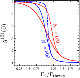
Figure 11: (Color online) Second order coherence function $g^{(2)}$ as we sweep through threshold. The solid red curve shows the results of a full numerical calculation of the probability distribution for $N=100$ while the red dashed curve shows the result of the calculation based on second order cumulants described in the text. The blue curves show similar results for $N=500$. The other parameters used are the same as those in Fig. 3 except we directly specify $\Gamma(-\delta)=1$GHz, $\Gamma(\delta)=50$MHz.

In Figure 11 we plot the value of $g^{(2)}$ calculated by solving the full master equation for both $N=100$ and $N=500$ and compare these with the results of the second moment calculation described above. For both calculations we see a crossover from $g^{(2)}=2$ to $g^{(2)}=1$ which becomes sharper as the number of molecules is increased. This is the same behaviour as is observed experimentally Schmitt et al. (2012).The two approaches match well above and at threshold, however, at small pumping strengths the crossover is not captured correctly by the second order cumulants. This is because below threshold the probability distribution of the system is far from Gaussian and so the approach based on truncating at second order breaks down.

As the number of molecules grows, the transition between $g^{(2)}=1$ and $g^{(2)}=2$ becomes increasingly sharp; this is seen by both the full probability distribution and the cumulant calculation. For $N=10^{9}$, the cumulant calculation predicts a very sharp transition at threshold. In comparing these results to the recent experiments Schmitt et al. (2014a) it should be noted that in this section we have considered a single-mode approximation; calculating the full non-equilibrium correlation function for a many mode system is a challenge for future work.

IV.2 Emission lineshape

To examine the temporal coherence of the emitted light source we can use a similar formalism to calculate the emission spectrum of the cavity Walls and Milburn (1994)

$$S_{\hat{a}^{\dagger}\hat{a}}(\omega)=2{\rm Re}\int_{0}^{\infty}dt\langle{\hat{a}^{\dagger}(t)\hat{a}(0)}\rangle{\rm e}^{i\omega t}.$$ (34)

From the quantum regression theorem Walls and Milburn (1994) we know that the equation of motion for this two-time correlation function is simply given by the evolution of $\hat{a}^{\dagger}(t)$ starting from the initial density matrix $\hat{\rho}(0)=\hat{a}\hat{\rho}_{ss}$ where $\hat{\rho}_{ss}$ is the stationary state. this means that we need to find the time evolution of

$$\langle{\hat{a}^{\dagger}(t)\hat{a}(0)}\rangle=\sum_{n,m}\sqrt{n}P^{1}_{n,m},$$ (35)

where $P^{1}_{n,m}$ represents the elements of the density matrix which are on the first off-diagonal in the photon number basis, and diagonal in number of excited molecules. These correspond to defining ${\hat{\rho}}=\sum_{n,m}P^{1}_{n,m}\ket{n-1}\bra{n}\otimes\rho_{m}$ in an analogous way to the definition of $P_{n,m}$ in the previous section. The equation for the evolution of this can be derived from the master equation in the same way as Eq. (27) and is given by

$$\dot{P}^{1}_{n,m}=\kappa[\sqrt{n(n+1)}P^{1}_{n+1,m}-(n-1/2)P_{n,m}^{1}]\\ +\Gamma_{\uparrow}[(N-m+1)P^{1}_{n,m-1}-(N-m)P^{1}_{n,m}]\\ +\Gamma_{\downarrow}[(m+1)P^{1}_{n,m+1}-mP^{1}_{n,m}]\\ +\Gamma(-\delta)\left[\sqrt{n(n+1)}(m+1)P^{1}_{n-1,m+1}-(n+1/2)mP^{1}_{n,m}\right]\\ +\Gamma(\delta)\left[\sqrt{n(n+1)}(N-m+1)P^{1}_{n+1,m-1}\right.\\ \left.\vphantom{\sqrt{n(n+1)}}-(n-1/2)(N-m)P^{1}_{n,m}\right].$$ (36)

Here we have ignored the Hamiltonian terms since these only shifts the origin of frequency in the power spectrum. The full problem then reduces to finding the time evolution of the above equation using the initial condition $P^{1}_{n,m}(0)=\sqrt{n}P_{n,m}^{\text{steady}}$. The same numerical techniques as before can be applied to this problem to find the emission spectrum.

In Figure 12 (a) and (b) we show the emission spectrum below and above threshold respectively, calculated numerically for $N=100$, along with Lorentzian fits to the data. We see that above threshold the lineshape is almost perfectly Lorentzian while below threshold there is some deviation at high frequencies, this is because below threshold there is a significant effect from the dynamics of the molecules on short timescales which causes the lineshape to deviate slightly. Above threshold, there is a significant separation of timescales, so that the slow exponential decay of correlations occurs on much longer timescales than the fast dynamics of the molecular state, and so the two can be clearly separated — note the frequency scales appearing in Fig. 12.

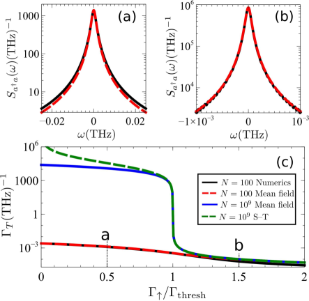
Figure 12: (Color online) The emission spectra below (a) and above (b) the transition point, calculated for $N=100$. The exact solution is shown as the solid (black) lines while the Lorentzian fits are shown as dashed (red) curves. Panel (c) shows the linewidth of the emission spectrum. In the small system size limit ($N=100$) we show the full numerics as the solid black line while the mean field approximation is given by the red dashed line. In the thermodynamic limit ($N=10^{9}$) we show the full mean field calculation as the blue solid line while the Schawlow–Townes result is the green dashed curve. The points marked a and b indicate the locations at which the spectra in the other panels were calculated. The other parameters used are the same as those in Fig. 3 except we directly specify $\Gamma(-\delta)=1$GHz, $\Gamma(\delta)=50$MHz.

As above, for large $N\simeq 10^{9}$, exact solution of Eq. (36) is no longer feasible. To find the linewidth in the thermodynamic limit we can however make a mean field approximation. This can be done by calculating an explicit expression for $\langle{\hat{a}^{\dagger}(t)\hat{a}(0)}\rangle$ from Eq. (35) and truncating the resulting evolution at the mean field level, i.e. assuming that $P^{1}_{n,m}\simeq P^{1}_{n}P_{m}$ can be factorized. We find for the correlation function

$$\frac{d}{dt}\langle{\hat{a}^{\dagger}(t)\hat{a}(0)}\rangle=-\left(\frac{\Gamma^{-}(t)}{2}-\frac{\Gamma^{+}(t)}{2}\right)\langle{\hat{a}^{\dagger}(t)\hat{a}(0)}\rangle.$$ (37)

where the rates are given by

$$\Gamma^{-}(t)=\kappa+\Gamma(\delta)(N-\langle{m}\rangle),$$ (38)

$$\Gamma^{+}(t)=\Gamma(-\delta)\langle{m}\rangle.$$ (39)

Here the coupling between the photonic and molecular degrees of freedom means that the rates which occur in this equation depend on the inversion of the molecules. This dependence encodes the short-time effects discussed above, whereby the state of the molecules is perturbed by the removal of one photon. It is therefore necessary to follow the evolution of $\langle{m(t)}\rangle$ from its initial steady state value, according to its equation of motion,

$$\dot{\langle{m}\rangle}={\Gamma}_{\uparrow}^{\rm tot}(t)(N-\langle{m}\rangle)-{\Gamma}_{\downarrow}^{\rm tot}(t)\langle{m}\rangle.$$ (40)

The rates in this expression depend on the current photon population:

$${\Gamma}_{\downarrow}^{\rm tot}=\Gamma_{\downarrow}+\Gamma(-\delta)(\langle{n}\rangle+1),$$ (41)

$${\Gamma}_{\uparrow}^{\rm tot}=\Gamma_{\uparrow}+\Gamma(\delta)\langle{n}\rangle,$$ (42)

and $\langle{n}\rangle$ evolves according to

$$\dot{\langle{n}\rangle}=-\Gamma^{-}(t)\langle{n}\rangle+\Gamma^{+}(t)(\langle{n}\rangle+1).$$ (43)

This then gives a closed set of equations for the evolution which can be used with the quantum regression theorem to calculate the correlation function.

As already noted earlier, above threshold there is a separation of timescales between the fast molecular dynamics and the slow decay of correlations. This means that for the purpose of finding an approximate expression for the lineshape above threshold, we may ignore the (fast) time dependence of the rates in Eq. (37) and simply using the steady state values. This gives rise to the Lorentzian spectrum

$$S_{\hat{a}^{\dagger}\hat{a}}(\omega)=\frac{2\langle{n}\rangle_{ss}\Gamma_{T}}{(\delta+\omega)^{2}+\Gamma_{T}^{2}},$$ (44)

where $\Gamma_{T}=[\Gamma^{-}(\infty)-\Gamma^{+}(\infty)]/2$ is the effective decay rate of the two-time correlation function evaluated in the steady state.

We can then use this calculation to look at the linewidth of the emission spectrum calculated using Eq. (34). An example of the way in which the width of the emission spectrum changes as the pump power is increased through the transition threshold is shown in Fig. 12 (c). For small particle numbers the full numerics agree very closely with the results of the mean field calculation with only a slight deviation above threshold where the variances become important. This then allows us to trust the results of the mean field calculation in the thermodynamic limit. For $N=10^{9}$ we see that below threshold the emission is very broad and weak. At the transition point the linewidth collapses and then saturates at a value which is controlled both by the losses from the cavity and the absolute value of the dye absorption and emission rates. The below threshold linewidth is controlled by the number of molecular exitations, in this limit there is no stimulated emission and the emission is broadened by the molecules.

Despite the excellent match to the linewidth, it is worth noting that the mean field model presented here cannot accurately calculate the full spectrum above threshold. In this limit the dynamics goes through a region where there are correlations between the photons and the molecules and hence the factorization of the cumulants is no longer valid, in this region the mean field model predicts unphysical negative spectral weight at some frequencies. Such considerations only effect the short time dynamics, and not the slow dynamics that determine the linewidth. The weight of the Lorentzian lineshape is however modified by this early time dynamics.

In the large photon number limit the linewidth given by $\Gamma_{T}$ ultimately takes the Schawlow–Townes Schawlow and Townes (1958); Scully and Zubairy (1997) form:

$$\Gamma_{T}=\frac{\kappa}{2}+\frac{N[\Gamma(\delta)\Gamma(-\delta)-\Gamma_{\uparrow}\Gamma(-\delta)+\Gamma_{\downarrow}\Gamma(\delta)]}{2n_{ss}[\Gamma(\delta)+\Gamma(-\delta)]}.$$ (45)

This is plotted alongside the mean field result in Fig. 12 as the dashed (green) line, we see good agreement in the condensed phase which breaks down, as expected, when the occupation of the photon mode is small.

V Conclusions

In this paper we have developed a quantum mechanical model capable of describing the thermalization of photons inside a dye-filled microcavity. We have shown how this model is able to predict the behavior of the recent experiments on photon Bose-Einstein condensation.

From our full quantum model we derived a rate equation capable of describing many features of the system. We were able to define a threshold condition which allows us to identify when the system transitions to a macroscopically occupied state. This was then used to investigate the breakdown of thermalization in the photon condensate. We showed how, by changing the length of the cavity, the low energy modes interact with the dye too weakly to thermalize and the Bose-Einstein description breaks down. We also looked at how, for extreme parameters of the dye, it is possible to make the system selectively thermalize only in certain frequency regimes. This led us to identify two possible criteria which can identify if the system is close to thermal equilibrium or not: the mode which gains a macroscopic occupation and the chemical potential of a Bose-Einstein distribution fit to the above threshold distribution. The phase diagrams of these criteria for thermalization as a function of temperature and parameters of the dye were then examined. We have investigated the way in which the system approaches a thermal equilibrium distribution by examining the dynamics as the pump is switched on.

We have also begun to explore the quantum correlations of such a system, going beyond the mean-field (i.e. rate equation) description. Using the full quantum model we have shown how one may calculate both the second order coherence of the emitted light and its linewidth.