We will describe the quantum statistical approach to parton distributions allowing to obtain simultaneously the unpolarized distributions and the helicity distributions. We will present some recent results, in particular related to the nucleon spin structure in QCD. Future measurements are challenging to check the validity of this novel physical framework.

Key words: Gluon polarization; Proton spin; Statistical distributions PACS numbers: PACS numbers: 12.40.Ee, 13.60.Hb, 13.88.+e, 14.70.Dj

1 Basic review on the statistical description

Let us first recall some of the basic components for building up the parton distribution functions (PDF) in the statistical approach, as oppose to the standard polynomial type parametrizations, based on Regge theory at low $x$ and counting rules at large $x$. The fermion distributions are given by the sum of two terms [1], the first one, a quasi Fermi-Dirac function and the second one, a flavor and helicity independent diffractive contribution equal for light quarks. So we have, at the input energy scale $Q_{0}^{2}$,

$$xq^{h}(x,Q^{2}_{0})=\frac{AX^{h}_{0q}x^{b}}{\exp[(x-X^{h}_{0q})/\bar{x}]+1}+\frac{\tilde{A}x^{\tilde{b}}}{\exp(x/\bar{x})+1}~{},$$ (1)

$$x\bar{q}^{h}(x,Q^{2}_{0})=\frac{{\bar{A}}(X^{-h}_{0q})^{-1}x^{\bar{b}}}{\exp[(x+X^{-h}_{0q})/\bar{x}]+1}+\frac{\tilde{A}x^{\tilde{b}}}{\exp(x/\bar{x})+1}~{}.$$ (2)

It is important to remark that $x$ is indeed the natural variable, and not the energy like in statistical mechanics, since all sum rules we will use are expressed in terms of $x$. Notice the change of sign of the potentials and helicity for the antiquarks. The parameter $\bar{x}$ plays the role of a universal temperature and $X^{\pm}_{0q}$ are the two thermodynamical potentials of the quark $q$, with helicity $h=\pm$. We would like to stress that the diffractive contribution occurs only in the unpolarized distributions $q(x)=q_{+}(x)+q_{-}(x)$ and it is absent in the valence $q_{v}(x)=q(x)-\bar{q}(x)$ and in the helicity distributions $\Delta q(x)=q_{+}(x)-q_{-}(x)$ (similarly for antiquarks). The nine free parameters to describe the light quark sector ($u$ and $d$), namely $X_{u}^{\pm}$, $X_{d}^{\pm}$, $b$, $\bar{b}$, $\tilde{b}$, $\tilde{A}$ and $\bar{x}$ in the above expressions, were determined at the input scale from the comparison with a selected set of very precise unpolarized and polarized Deep Inelastic Scattering (DIS) data [1]. The additional factors $X_{q}^{\pm}$ and $(X_{q}^{\pm})^{-1}$ come from the transverse momentum dependence (TMD), as explained in Refs. [2,3] (See below). For the gluons we consider the black-body inspired expression

$$xG(x,Q^{2}_{0})=\frac{A_{G}x^{b_{G}}}{\exp(x/\bar{x})-1}~{},$$ (3)

a quasi Bose-Einstein function, with $b_{G}$, the only free parameter, since $A_{G}$ is determined by the momentum sum rule. We also assume a similar expression for the polarized gluon distribution $x\Delta G(x,Q^{2}_{0})={\tilde{A}}_{G}x^{{\tilde{b}}_{G}}/[\exp(x/\bar{x})-1]$. For the strange quark distributions, the simple choice made in Ref. [1] was greatly improved in Ref. [4]. Our procedure allows to construct simultaneously the unpolarized quark distributions and the helicity distributions. This is worth noting because it is a very unique situation. Following our first paper in 2002, new tests against experimental (unpolarized and polarized) data turned out to be very satisfactory, in particular in hadronic collisions, as reported in Refs. [5,6].

2 Some selected recent preliminary results

Since 2002 a lot of new DIS data have been published and although our early determination of the PDF has been rather successful, which reflects the fact this physical approach lies on solid grounds, we felt that it was timely to revisit it.
We have slightly increased the number of free parameters, in particular to describe the strange quark distributions, and these parameters were determined from a next-to leading order (NLO) fit of a large set of accurate DIS data, (the unpolarized structure functions $F_{2}^{p,n,d}(x,Q^{2})$, the polarized structure functions $g_{1}^{p,n,d}(x,Q^{2})$, the structure function $xF_{3}^{\nu N}(x,Q^{2})$ in $\nu N$ DIS, etc…) a total of 2140 experimental points. Although the full details of these new results in their final form will be presented in a forthcoming paper [7], we just want to make a general remark. By comparing with the results of 2002 [1], we have observed, so far, a remarquable stability of some important parameters, the light quarks potentials $X_{0u}^{\pm}$ and $X_{0d}^{\pm}$, whose numerical values are almost unchanged. The new temperature is slightly lower. As a result the main features of the new light quark and antiquark distributions are only hardly modified, which is not surprizing, since our 2002 PDF set has proven to have a rather good predictive power.

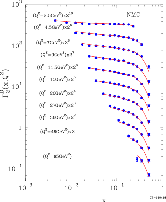
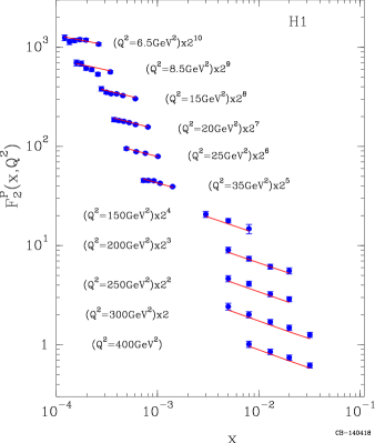
Figure 1: Left : Comparison of the data on $F_{2}^{D}(x,Q^{2})$ from NMC [8], with the predictions of the statistical model (solid curves). Right : Comparison of some selected data on $F_{2}^{p}(x,Q^{2})$ from H1 [9], with the predictions of the statistical model (solid curves).

First we present some selected experimental tests for the unpolarized PDF by considering $\mu N$ and $eN$ DIS, for which several experiments have yielded a large number of data points on the structure functions $F_{2}^{N}(x,Q^{2})$, $N$ stands for either a proton or a deuterium target. We have used fixed target measurements which cover a rather limited kinematic region in $Q^{2}$ and $x$ and also HERA data which cover a very large $Q^{2}$ range and probe the very low $x$ region, dominated by a fast rising behavior, consistent with our diffractive term (See Eq. (1)).
For illustration of the quality of our fit and, as an example, we show in Fig. 1, our results for $F_{2}^{D}(x,Q^{2})$ with NMC data on a deuterium target and for $F_{2}^{p}(x,Q^{2})$ with H1 data on a proton target. We note that the analysis of the scaling violations leads to a gluon distribution $xG(x,Q^{2})$, in fairly good agreement with our simple parametrization (See Eq. (3)).

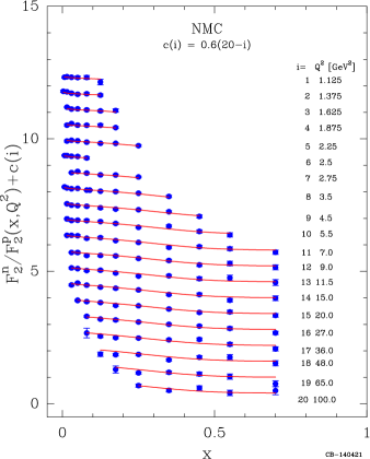
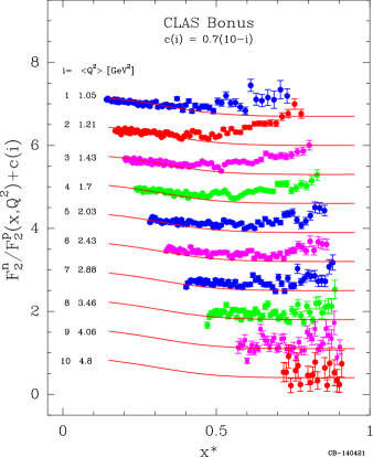
Figure 2: Left : Comparison of the data on $F_{2}^{n}/F_{2}^{p}(x,Q^{2})$ from NMC [10], with the predictions of the statistical model (solid curves). Right : Comparison of the data on $F_{2}^{n}/F_{2}^{p}(x,Q^{2})$ from CLAS [11], with the predictions of the statistical model (solid curves).

Another rather interesting physical quantity is the neutron $F_{2}^{n}$ structure function and in particular the ratio $F_{2}^{n}/F_{2}^{p}(x,Q^{2})$ which provides strong contraints on the PDF of the nucleon. For example the behavior of this ratio at large $x$ is directly related to the ratio of the $d$ to $u$ quarks in the limit $x\to 1$, a long standing-problem for the proton structure. We show in Fig. 2 the results of two experiments, NMC (Left) which is very accurate and covers a reasonnable $Q^{2}$ range up to $x=0.7$ and CLAS (Right) which covers a smaller $Q^{2}$ range up to larger $x$ values, both are fairly well described by the statistical approach. Several comments are in order. In the small $x$ region this ratio, for both cases, tends to 1 because the structure functions are dominated by sea quarks driven by our universal diffractive term. In the high $x$ region dominated by valence quarks, the NMC data suggest that this ratio goes to a value of the order of 0.4 for $x$ near 1, which corresponds to the value 0.16 for $d(x)/u(x)$ when $x\to 1$, as found in the statistical approach [6]. The CLAS data at large $x$ cover the resonance region of the cross section and an important question is whether Bloom-Gilman duality holds as well for the neutron as it does for the proton. We notice that the predictions of the statistical approach suggest an approximate validity of this duality, except for some low $Q^{2}$ values. A better precision and the extension of this experiment with the 12GeV Jefferson Lab will certainly provide even stronger constraints on PDFs up to $x\simeq 0.8$.

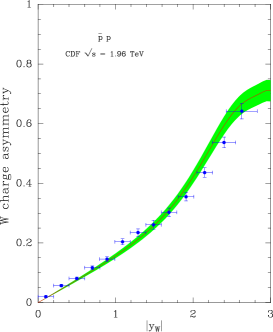
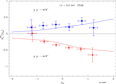
Figure 3: Left : The measured W production charge asymmetry from CDF [12] versus the W rapidity $y_{W}$ and the prediction from the statistical approach (solid line). The shaded band represents the uncertainties with a CL of 68%. Right : The measured parity-violating helicity asymmetries $A_{L}^{PV}$ for charged-lepton production at RHIC-BNL from STAR [13], through production and decay of $W^{\pm}$ versus $y_{e}$, the charged-lepton rapidity. The solid curves are the predictions from the statistical approach.

Let us now turn to the very interesting process of $W^{\pm}$ production in hadronic collisions. We recall that the differential cross section in $pp$ collision $\sigma^{W^{\pm}}(y)$, where $y$ is the rapidity of the $W^{\pm}$, can be computed directly from the Drell-Yan process dominated by quark-antiquark fusion, $u\bar{d}\to W^{+}$ and $\bar{u}d\to W^{-}$.

The charge asymmetry defined as

$$A(y)=[\sigma^{W^{+}}(y)-\sigma^{W^{-}}(y)]/[\sigma^{W^{+}}(y)+\sigma^{W^{-}}(y)]~{},$$ (4)

contains valuable information on the light quarks distributions inside the proton and in particular on the ratio down-to-up quark. A direct measurement of this asymmetry has been achieved by CDF at FNAL-Tevatron [12] and the results are shown in Fig. 3 (Left). The agreement with the predictions of the statistical approach is good and we note that in the high-$y$ region, $A(y)$ tends to flatten out, following the behavior of the predicted $d(x)/u(x)$ in the high-$x$ region.
Next we consider the process $\overrightarrow{p}p\to W^{\pm}+X\to e^{\pm}+X$, where the arrow denotes a longitudinally polarized proton and the outgoing $e^{\pm}$ have been produced by the leptonic decay of the $W^{\pm}$ boson. The helicity asymmetry is defined as

$$A_{L}^{PV}=\frac{d\sigma_{+}-d\sigma_{-}}{d\sigma_{+}+d\sigma_{-}}~{}.$$ (5)

Here $\sigma_{h}$ denotes the cross section where the initial proton has helicity $h$. It was measured recently at RHIC-BNL [13] and the results are shown in Fig. 3 (Right). As explained in Ref. [14], the $W^{-}$ asymmetry is very sensitive to the sign and magnitude of $\Delta\bar{u}$, so this is another successful result of the statistical approach.

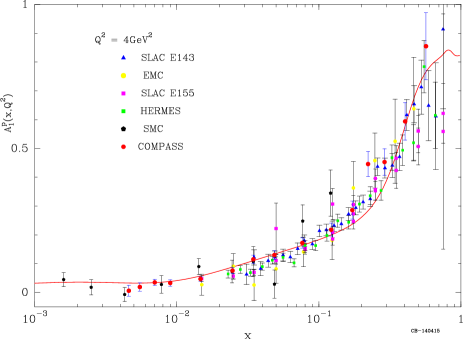
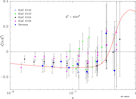
Figure 4: Top : Comparison of the world data on $A_{1}^{p}(x,Q^{2})$ at $Q^{2}=4\mbox{GeV}^{2}$, with the result of the statistical approach. Bottom : Comparison of the world data on $A_{1}^{n}(x,Q^{2})$ at $Q^{2}=4\mbox{GeV}^{2}$, with the result of the statistical approach.

Finally we turn to the important issue concerning the asymmetries $A_{1}^{p,d,n}(x,Q^{2})$, measured in polarized DIS. We recall the definition of the asymmetry $A_{1}(x,Q^{2})$, namely

$$A_{1}(x,Q^{2})=\frac{(g_{1}(x,Q^{2})-\gamma^{2}(x,Q^{2})g_{2}(x,Q^{2}))2x[1+R(x,Q^{2})]}{[1+\gamma^{2}(x,Q^{2})]F_{2}(x,Q^{2})}~{},$$ (6)

where $g_{1,2}(x,Q^{2})$ are the polarized structure functions, $\gamma^{2}(x,Q^{2})=4M^{2}x^{2}/Q^{2}$ and $R(x,Q^{2})$ is the ratio between the longitudinal and transverse photoabsorption cross sections. We display in Fig. 4 the world data on $A_{1}^{p,n}(x,Q^{2})$ at $Q^{2}=4\mbox{GeV}^{2}$, with the results of the statistical approach.

Note that these asymmetries do NOT reach 1 when $x\to 1$ as required by the counting rules prescription, which we don’t impose.
Finally one important outcome of this new analysis of DIS data in the framework of the statistical approach, is the discovery of a large gluon helicity distribution. When this talk was delivered, we had obtained a preliminary determination of $x\Delta G(x,Q^{2})$ which has been improved very recently and for more details we refer the reader to Ref. [15].

3 Transverse momentum dependence of the parton distributions

The parton distributions $p_{i}(x,k^{2}_{T})$ of momentum $k_{T}$, must obey the momentum sum rule $\sum_{i}\int_{0}^{1}dx\int xp_{i}(x,k^{2}_{T})dk^{2}_{T}=1$. In addition it must also obey the transverse energy sum rule $\sum_{i}\int_{0}^{1}dx\int p_{i}(x,k^{2}_{T})\frac{k^{2}_{T}}{x}dk^{2}_{T}=M^{2}$. From the general method of statistical thermodynamics we are led to put $p_{i}(x,k^{2}_{T})$ in correspondance with the following expression $\exp({\frac{-x}{\bar{x}}}+{\frac{-k^{2}_{T}}{x\mu^{2}}})$ , where $\mu^{2}$ is a parameter interpreted as the transverse temperature. So we have now the main elements for the extension to the TMD of the statistical PDF. We obtain in a natural way the Gaussian shape with no $x,k_{T}$ factorization, because the quantum statistical distributions for quarks and antiquarks read in this case

$$xq^{h}(x,k_{T}^{2})=\frac{F(x)}{\exp(x-X^{h}_{0q})/\bar{x}+1}\frac{1}{\exp(k^{2}_{T}/x\mu^{2}-Y^{h}_{0q})+1}~{},$$ (7)

$$x\bar{q}^{h}(x,k_{T}^{2})=\frac{{\bar{F}}(x)}{\exp(x+X^{-h}_{0q})/{\bar{x}}+1}\frac{1}{\exp(k^{2}_{T}/x\mu^{2}+Y^{-h}_{0q})+1}~{}.$$ (8)

Here $F(x)=\frac{Ax^{b-1}X^{h}_{0q}}{\ln{(1+\exp{Y^{h}_{0q}})}\mu^{2}}=\frac{Ax^{b-1}}{k\mu^{2}}$, where $Y^{h}_{0q}$ are the thermodynamical potentials chosen such that $\ln{(1+\exp{Y^{h}_{0q}})}=kX^{h}_{0q}$, in order to recover the factors $X^{h}_{0q}$ and $(X^{h}_{0q})^{-1}$, introduced earlier.
Similarly for $\bar{q}$ we have $\bar{F}(x)=\bar{A}x^{2b-1}/k\mu^{2}$. The determination of the 4 potentials $Y^{h}_{0q}$ can be achieved with the choice $k=3.05$. Finally $\mu^{2}$ will be obtained from the transverse energy sum rule and one finds $\mu^{2}=0.198\mbox{GeV}^{2}$. Detailed results are shown in Refs. [2,3]. Before closing we would like to mention an important point. So far in all our quark or antiquark TMD distributions, the label ”‘$h$”’ stands for the helicity along the longitudinal momentum and not along the direction of the momentum, as normally defined for a genuine helicity. The basic effect of a transverse momentum $k_{T}\neq 0$ is the Melosh-Wigner rotation, which mixes the components $q^{\pm}$ in the following way $q^{+MW}=\cos^{2}\theta~{}q^{+}+\sin^{2}\theta~{}q^{-}~{}~{}~{}\mbox{and}~{}~{}~{}q^{-MW}=\cos^{2}\theta~{}q^{-}+\sin^{2}\theta~{}q^{+}$, where for massless partons, $\theta=\arctan{(\frac{k_{T}}{p_{0}+p_{z}})}$, with $p_{0}=\sqrt{k_{T}^{2}+p_{z}^{2}}$. It vanishes when either $k_{T}=0$ or $p_{z}$, the quark longitudinal momentum, goes to infinity. Consequently $q=q^{+}+q^{-}$ remains unchanged since $q^{MW}=q$, whereas we have $\Delta q^{MW}=(\mbox{cos}^{2}\theta-\mbox{sin}^{2}\theta)\Delta q$.

References

- [1] C. Bourrely, F. Buccella and J. Soffer, Eur. Phys. J. C23, 487 (2002).
- [2] C. Bourrely, F. Buccella and J. Soffer, Phys. Rev. D83, 074008 (2011).
- [3] C. Bourrely, F. Buccella and J. Soffer, Int. J. of Modern Physics A28, 1350026 (2013).
- [4] C. Bourrely, F. Buccella and J. Soffer, Phys. Lett. B648, 39 (2007).
- [5] C. Bourrely, F. Buccella and J. Soffer, Mod. Phys. Lett. A18, 771 (2003).
- [6] C. Bourrely, F. Buccella and J. Soffer, Eur. Phys. J. C41, 327 (2005).
- [7] C. Bourrely, F. Buccella and J. Soffer, in preparation.
- [8] NMC Collaboration, M. Arneodo et al., Nucl. Phys. 483, 3 (1997).
- [9] H1 Collaboration, C. Adloff et al., Nucl. Phys. 497, 3 (1997); Eur. Phys. J. C13, 609 (2000); Eur. Phys. J. C21, 33 (2001)
- [10] NMC Collaboration, P. Amaudruz et al., Phys. Rev. Lett. 66, 2712 (1991).
- [11] CLAS Collaboration, N. Baillie et al., Phys. Rev. Lett. 108, 142001 (2012), Erratum-ibid, 108, 199902 (2012).
- [12] CDF Collaboration, T. Aaltonen et al., Phys. Rev. Lett. 102, 181801 (2009).
- [13] STAR Collaboration, L. Adamczyk et al., Phys. Rev. Lett. 113, 072301 (2014).
- [14] C. Bourrely, F. Buccella and J. Soffer, Phys. Lett. B726, 296 (2013).
- [15] C. Bourrely and J. Soffer, arXiv:1408.7057 [hep-ph], submitted for publication in Physics Letters B.