The Near-Ultraviolet Luminosity Function of Young, Early M-Type Dwarf Stars

Abstract

Planets orbiting within the close-in habitable zones of M dwarf stars will be exposed to elevated high-energy radiation driven by strong magneto-hydrodynamic dynamos during stellar youth. Near-ultraviolet (NUV) irradiation can erode and alter the chemistry of planetary atmospheres, and a quantitative description of the evolution of NUV emission from M dwarfs is needed when modeling these effects. We investigated the NUV luminosity evolution of early M-type dwarfs by cross-correlating the Lépine & Gaidos (2011) catalog of bright M dwarfs with the GALEX catalog of NUV (1771–2831Å) sources. Of the 4805 sources with GALEX counterparts, 797 have NUV emission significantly ($>2.5\sigma$) in excess of an empirical basal level. We inspected these candidate active stars using visible-wavelength spectra, high-resolution adaptive optics imaging, time-series photometry, and literature searches to identify cases where the elevated NUV emission is due to unresolved background sources or stellar companions; we estimated the overall occurrence of these “false positives” as $\sim$16%. We constructed a NUV luminosity function that accounted for false positives, detection biases of the source catalogs, and GALEX upper limits. We found the NUV luminosity function to be inconsistent with predictions from a constant star-formation rate and simplified age-activity relation defined by a two-parameter power law.

myfnsymbols††‡‡

1. INTRODUCTION

The characteristics of M dwarf stars make them favorable targets in the search for Earth-like planets. Their “habitable zones” (i.e., the range of orbital semi-major axes at which liquid water is stable on an Earth-like planet) are more compact than those of solar-type stars due to their comparatively low luminosities. These closer orbits make Earth-like planets possible to detect with radial velocity and transit methods (Tarter et al., 2007; Scalo et al., 2007; Gaidos et al., 2007).

However, planets in the close-in habitable zones of M dwarfs may be exposed to elevated levels of high-energy radiation. The photospheres of M dwarfs emit negligibly at short wavelengths due to low effective temperatures and absorption by neutral iron (Fe I). Yet these stars can emit ultraviolet (UV) and X-ray radiation from their upper chromospheres, coronae, and active regions due to heating from their strong magnetic-hydrodynamic dynamos.

UV radiation may play opposing roles in planet habitability and the origins of life. Elevated UV radiation can irreparably damage organisms on planetary surfaces as well as erode planetary atmospheres by injecting heat that drives escape of hydrogen and other volatiles required for life (e.g., Tian, 2009; Erkaev et al., 2013; Miguel et al., 2014). On the other hand, atmospheric UV photochemistry is a potential source of prebiotic molecules (Ehrenfreund et al., 2002) and UV radiation can induce mutations upon which natural selection can act (e.g., Rotchschild, 1999). Buccino et al. 2006 defined the “UV habitable zone” as the distance at which a planet is close enough to receive sufficient UV radiation to enable biogenesis processes, but also far enough to avoid irreparable damage to DNA by exposure to heightened levels of UV flux. Buccino et al. 2007 derived the UV habitable zones for three planet-hosting M dwarfs (GJ 581, GJ 849, GJ 876) with UV spectra from the International Ultraviolet Explorer (IUE). They found that for all three systems the liquid-water and UV habitable zones did not overlap, and suggested that an alternative source of UV emission, such as stellar flares, might be needed to enable prebiotic chemistry on planets orbiting in the liquid-water habitable zones around M dwarfs.

The UV emission of M dwarfs is known to evolve with age. Young M dwarfs ($\lesssim 100$ Myr) exhibit rapid rotation with strong magneto-hydrodynamic dynamos that result in enhanced UV (as well as X-ray) emission. As stars age, angular momentum is gradually lost through stellar winds, causing stars to spin down and become less active with time. Single early-M dwarfs (M0-M3) remain rapidly rotating and active for $\sim$1 Gyr, while many late-M dwarfs (M5-M9) stay in this state for up to $\sim$8 Gyr (West et al., 2008; Rebassa-Mansergas et al., 2013). This dichotomous behavior may result from the appearance of fully convective interiors and low Rossby numbers near the M4 spectral subtype (Reiners 2012; Gastine et al. 2013; see also Reiners & Mohanty 2012 for an alternative explanation for this dichotomy). Due to survey biases, the vast majority of known planet-hosting M dwarfs have early spectral subtypes. A quantitative description of the evolution of UV emission from early-M dwarfs is therefore important for accurately modeling the effects of UV irradiation on planets orbiting these stars (e.g., Miguel et al., 2014). Moreover, future exoplanet surveys—such as K2, the Transiting Exoplanet Survey Satellite (TESS; Ricker, 2014), and the Next Generation Transit Survey (NGTS; Wheatley et al., 2013)—will continue to monitor early-M dwarfs. These surveys will generate substantial data on the variability and rotation of these stars, which can then be compared to their UV emission.

Much of the UV emission from astronomical objects must be observed from space due to absorption by the Earth’s atmosphere at these short wavelengths. The Galaxy Evolution Explorer (GALEX; Martin et al. 2005) is a recently decommissioned space-based telescope that performed all-sky imaging in both near-UV (NUV; 1771–2831Å) and far-UV (FUV; 1344–1768Å) bandpasses (Figure 1). Several recent studies have used GALEX data to identify active and/or young M dwarfs (Browne et al., 2009; Rodriguez et al., 2011; Shkolnik et al., 2011; Rodriguez et al., 2013; Stelzer et al., 2013). Most notably, Stelzer et al. (2013) studied a volume-limited sample of 159 field M dwarfs within 10 pc, which they identified by cross-correlating the Lépine & Gaidos 2011 (hereafter LG11) catalog of bright M dwarfs with the GALEX sixth data release (GR6). They compared their sample to members of the TW Hydra young moving group (YMG), which has a known age of $\sim$10 Myr, to derive a power-law age-activity relation. They found that the UV luminosities of early-M dwarfs decline by roughly three orders of magnitude from $\sim$10 Myr to a few Gyr of age.

However, the Stelzer et al. (2013) sample was too small to quantitatively describe a UV luminosity function, particularly at higher UV luminosities where there are fewer stars. Furthermore, M dwarfs can appear UV luminous for reasons other than stellar youth. Such reasons include: unrelated background UV sources confused in the $\sim$5 arcsec beam of GALEX; companion white dwarfs or late-M dwarfs with persistent UV emission; or tidally locked binaries in which spin-orbit synchronization induces ongoing activity. These “false positives” (FPs) must be identified and removed, at least in a statistical sense, in order to estimate a UV luminosity function.

In this work we utilize the entire LG11 catalog of bright M dwarfs, cross-correlating it with the final version of the GALEX all-sky UV source catalog (GR7), to derive a NUV luminosity function (NUVLF) for early-M dwarfs (M0-M3). We describe our sample selection in Section 2 and detail our follow-up observations in Section 3. In Section 4 we describe our methods for identifying FPs and then estimate the overall FP rate in our sample using a maximum likelihood method. We construct the NUVLF in Section 5 by accounting for FPs, the detection biases of the source catalogs, and GALEX upper limits. In Section 6, we compare the NUVLF to simple models of star formation and M dwarf activity evolution as well as describe the implications and caveats of our findings.

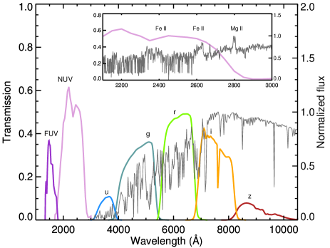
Figure 1.— GALEX FUV and NUV bandpasses compared to SDSS optical filters ($ugriz$). A PHOENIX model spectrum of an M dwarf with $T_{eff}=3700$ K and solar metallicity is plotted for reference (gray curve). The inset shows the NUV spectrum of an active, planet-hosting M dwarf (GJ 876; France et al., 2013) with the GALEX NUV bandpass (not to same scale) and activity-related emission lines shown for reference.

2. SAMPLE

2.1. Identifying M Dwarfs in the GALEX Catalog

We cross-correlated the LG11 catalog of 8889 nearby (${\rm d}\lesssim 60$ pc), bright ($J<10$), K7–M5 stars with the final GALEX data release (GR7). We searched the GALEX All-sky Imaging Survey (AIS), which contains both NUV and FUV sources, but kept only NUV matches as GALEX was much more sensitive in this bandpass (e.g., a preliminary cross-correlation by LG11 found five times more matches to NUV than FUV sources).

Our cross-correlation included a correction for stellar proper motion between the J2000 epoch of LG11 and the epochs of the individual GALEX AIS observations. We used the GalexView online tool to perform a preliminary cross-correlation between the LG11 and GALEX AIS catalogs with a 1 arcmin match radius. This search radius accounted for the resolution of GALEX ($\sim$5 arcsec) plus the maximum proper motion of any LG11 star over 10 years (roughly the time between the J2000 epoch and the last GALEX AIS observation). This preliminary search returned multiple GALEX AIS source matches for most LG11 stars, as expected from the large search radius. For each LG11 star we calculated its expected position on the sky at the observation date of each of its GALEX AIS matches. We then re-performed the cross-correlation using the adjusted LG11 positions and a reduced matching criterion of 5 arcsec (the resolution of GALEX) to identify the final source matches.

There were 1251 LG11 stars with multiple matches to the GALEX AIS catalog, even after correcting for proper motion and applying the stricter 5 arcsec search radius. For these we simply took the closest match. This was justified because almost all of these multiple matches were due to repeated GALEX AIS observations of a given area of sky: the matches had different GALEX AIS tile numbers and/or different exposure times, and thus are likely the same star. However there were 49 multiple matches that had the same GALEX tile number and exposure time, therefore representing the case when two objects are close enough on the sky to be confused by GALEX. The NUV magnitude differences for these 49 multiple matches were only $\sim$0.30 on average, and just 8 of these sources were ultimately used in the NUVLF. Thus the choice of which source to match should not significantly affect our derived NUVLF. Figure 2 compares the cross-correlation results before and after proper motion correction: the proper motion correction significantly improved the cross-correlation results, adding $\sim$300 new matches compared to the number of matches prior to proper motion correction, and significantly decreasing the residual angular separations of the matches, as illustrated by the histogram shift toward smaller offsets.

This cross-correlation process identified 5267 LG11 stars with NUV counterparts in the GALEX AIS catalog. Figure 3 plots $m_{\rm NUV}-K_{\rm S}$, a distant-independent measure of NUV luminosity, vs. $V-J$, a proxy for stellar effective temperature, for this sample. $m_{\rm NUV}$ is from the GALEX AIS catalog, $J$ and $K_{\rm S}$ are from the Two Micron All Sky Survey (2MASS; Skrutskie et al., 2006), and $V$ is from the AAVSO Photometric All-Sky Survey (APASS; Henden et al., 2012), the Tycho-2 and Hipparcos catalogs (Perryman & ESA, 1997), or generated from USNO-B magnitudes (Lépine & Shara, 2005).

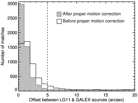
Figure 2.— Improved cross-correlation between LG11 and GALEX AIS catalogs after proper motion correction. The dashed line shows our match criteria of $\lesssim$ 5 arcsec separation (corresponding to the angular resolution of GALEX). After proper motion correction, the number of matches increased by $\sim$300 and the residual angular separations significantly decreased, as shown by the shift toward smaller offsets.

2.2. Determining the Basal NUV Locus

Most sources in Figure 3 fall along a locus (designated by gray points according to the criterion described below), which we interpret as the basal level of NUV emission for early-M dwarfs. To describe this basal NUV emission as a function of stellar effective temperature, we fit a line to median values of $m_{\rm NUV}-K_{\rm S}$ vs. $V-J$ using only stars with errors <10% in all bands and $V-J$ colors $<3.5$. We iteratively removed outlier stars and re-performed the fit until the remaining stars were Gaussian-distributed in $m_{\rm NUV}-K_{S}$ about the median-fit line. This gave a best-fit (designated by the black dashed line in Figure 3) with the following parameters:

$$m_{\rm NUV}-K_{\rm S}=7.72+1.66(V-J)$$ (1)

This basal NUV locus is presumably an extension of the locus of inactive solar-type stars, which reaches $m_{\rm NUV}-K_{\rm S}\sim 10$ at $V-J\sim 2$ (see Figure 2 in Findeisen et al., 2011). However, our basal locus is much bluer than predicted by PHOENIX model spectra (Allard et al., 2013; Rajpurohit et al., 2013) using solar abundances (Caffau et al., 2011) and log $g=5.0$. Thus this locus likely does not exclusively represent photospheric NUV emission. It also cannot be an artifact of a constant GALEX flux limit, as the lower right-hand region of Figure 3 is populated while the lower left-hand region is not. Instead, this locus likely indicates persistent NUV line emission from a higher-temperature upper chromosphere. Stelzer et al. (2013) previously noted that all M dwarfs appear to exhibit NUV emission in excess of their expected photospheric value from stellar atmosphere models.

2.3. Selecting the NUV-Luminous Stars

The distribution in Figure 3 also features a smaller population of stars with NUV emission significantly in excess of the empirically determined basal value. We interpret these NUV-luminous sources as being mostly young stars exhibiting heightened activity, but also including “false positives” that appear active for reasons other than stellar youth. We identified the 1210 NUV-luminous stars from the 5267 NUV-detected stars as those with $m_{\rm NUV}-K_{\rm S}$ colors at least $2.5\sigma$ ($\sim$1.12 magnitudes) bluer than their expected basal value given by Equation 1. We identify these stars as blue points in Figure 3.

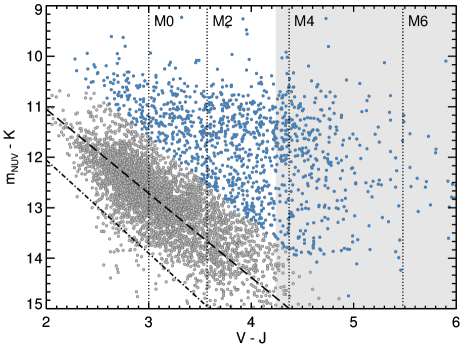
Figure 3.— LG11 stars with NUV counterparts in the GALEX AIS catalog. The $y$-axis is a measure of NUV luminosity and the $x$-axis is a proxy for stellar effective temperature that correlates to spectral subtype. The dominant locus (gray points) likely represents older M dwarfs, while the distinct population toward higher NUV luminosities (blue points) presumably represents young/active stars. Approximate spectral subtypes are shown for reference; stars later than M3 (indicated by the shaded region) were ultimately removed from our sample (see Section 2.4). The black dashed-dotted line shows the predicted photospheric level of NUV emission from PHOENIX model spectra. The dominant locus of older stars exhibits higher NUV emission than the predicted photospheric values, suggesting that all M dwarfs exhibit a basal level of NUV emission from their chromospheres. The median fit to this basal emission level is shown by the black dashed line and given in Equation 1.

2.4. Removing Late-M Dwarfs

We only consider early-M dwarfs (M0-M3) in the remainder of this work. This is because we identify our sample of young M dwarfs by their heightened UV luminosity (see Section 2.3), a property that has been observed to evolve significantly with stellar age for early-M dwarfs and at a much slower rate for late-M dwarfs (M5-M9). Namely, observations indicate that early-M dwarfs are rapidly rotating and active for only $\sim$1 Gyr, while late-M dwarfs remain in this state for up to $\sim$8 Gyr (West et al., 2008; Rebassa-Mansergas et al., 2013). This difference may be due to the transition to fully convective interiors around the M4 spectral subtype (Reiners, 2012; Gastine et al., 2013). We therefore removed stars with spectral subtypes later than M3 as a first step to ensuring our measured NUV excess is due to stellar youth rather than a longer duration of stellar activity.

To identify late-M dwarfs we used the empirical relation between $V-J$ color and spectral subtype derived in LG11 and then revised in Lépine et al. (2013) (see their Equation 12). These color-based assignments provide only rough estimates ($\pm$ 1 spectral subtype), however they also provide a uniform method of spectral classification, which is important for statistical studies such as this. Moreover, a rough estimate is sufficient because we are using these spectral subtypes to identify late-M dwarfs and the spectral subtype boundary between early- and late-M dwarfs is not well defined (i.e., somewhere between M3 and M5).

Removing the late-M dwarfs from our original sample of NUV-detected M dwarfs (see Section 2.1) resulted in a final sample of 4805 NUV-detected early-M dwarfs of which 797 were identified as NUV-luminous (see Section 2.3). All references hereafter to our “sample” are to this final selection that includes only early-M dwarfs, unless explicitly stated otherwise. Parameters of the NUV-luminous sources are presented in Table 4.

2.5. Characterizing the Basal NUV Locus

Figure 3 suggests that the locus of stars exhibiting basal NUV emission (gray points; see Section 2.1) has an intrinsic width. We estimated this intrinsic width by first taking the standard deviation of distances in $m_{\rm NUV}-K_{\rm S}$ from the locus median (black dashed line) to all stars in the locus with errors <10% in all bands. We accounted for measurement errors by subtracting in quadrature the median measurement errors for each band: the $m_{\rm NUV}$ errors were taken from the GALEX AIS catalog, the $V$-band errors were taken from the respective catalogs (see Section 2.1), and the $K_{\rm S}$- and $J$-band errors were considered negligible at <1%. Errors in $V-J$ were translated to $m_{\rm NUV}-K_{\rm S}$ using the slope of our median fit to the locus (see Equation 1) before subtracting in quadrature. We found that the locus of stars exhibiting basal NUV emission in Figure 3 has an intrinsic width of $\sim$0.50 magnitudes in $m_{\rm NUV}-K_{\rm S}$, after accounting for measurement errors.

The locus width could be the product of several factors, in particular stellar variability, interstellar extinction, unresolved binaries, and metallicity variations. We first investigated stellar variability using the 1202 LG11 stars in our sample with multiple matches to the GALEX AIS catalog that were likely repeated observations of the same star at different epochs rather than source confusion (see Section 2.1). We found the maximum difference in NUV magnitude for each multiple match, then took the standard deviation as an estimate of the error introduced by stellar variability. We then subtracted this value ($\sim$$0.24$) in quadrature along with the measurement errors (see above), which reduced the estimated intrinsic locus width by only $\sim$0.07 magnitudes. This shows that stellar variability is not a significant contributor to the locus width.

We also confirmed that the locus width was not due to interstellar extinction, $A(V)$. UV sources are subject to significant interstellar extinction, as evident by the significant drop in GALEX detections near the Galactic plane (see Figure 1 in Bianchi et al., 2011). However, interstellar extinction should be negligible for our sample as most LG11 stars reside within 60 pc and are therefore contained within a low-density ($\sim$0.005 atoms cm^-3) region known as the “Local Bubble” (Cox & Reynolds, 1987). Nevertheless, we tested whether interstellar extinction could account for the locus scatter by searching for a minimum locus width as a function of assumed extinction per parsec, as described below. We found distances to each star using the $J$-band photometric distance, where M_J was obtained from $V-J$ color (although LG11 computes photometric distances, we re-compute them here using an updated color magnitude relation given by Equation 22 in Lépine et al. 2013). We used extinction coefficients from Yuan et al. (2013), which produced reddening corrections of E${}_{(NUV-K)}=2.24\times A(V)$ and E${}_{(V-J)}=0.77\times A(V)$. We tested $A(V)$ values ranging from 0 to 0.001 mag pc^-1 at a cadence of $1.5\times 10^{-6}$ mag pc^-1. This encompassed values well beyond the expected interstellar extinction within 60 pc; assuming $A(V)\sim 1$ mag kpc^-1 along the Galactic plane, and conservatively assuming a Local Bubble that is 10% the typical density of the interstellar medium, the expected interstellar extinction within 60 pc is $A(V)\sim 0.0001$ mag pc^-1. We applied reddening corrections to each star based on their individual distances, then re-measured the locus width for each $A(V)$ test value. We found no local minimum in the locus scatter. Rather, attempting to correct for extinction only increased the scatter of the locus.

We therefore concluded that stellar variability and interstellar extinction do not contribute significantly to the locus width. However, the locus width may be due to unresolved binaries, metallicity-dependent stellar colors, and continued variation of the basal NUV emission level with age. Unfortunately our dataset did not allow us to investigate these possibilities in detail.

2.6. Comparing FUV & X-ray Emission

We checked for FUV and X-ray counterparts to our sample. To obtain FUV counterparts we simply took the FUV sources associated with our NUV matches to the GALEX AIS catalog. To identify stars with X-ray counterparts, we cross-correlated our sample with the ROSAT All-Sky Survey Bright Source Catalog (Voges et al., 1999) and Faint Source Catalog (Voges et al., 2000). We used a 25 arcsec search radius around the LG11 coordinates, corresponding to the 2$\sigma$ ROSAT positional uncertainty determined by Voges et al. (1999). We converted the PSPC detector count rate into an X-ray flux, F_X, using the conversion factor from Schmitt et al. (1995): ${\rm CF}=(5.30{\rm HR}+8.31)10^{-12}$ ergs cm^-2 count^-1 where HR is the first hardness ratio from the ROSAT catalog. We did not correct for proper motion for this cross-correlation due to the large positional uncertainty of ROSAT compared to GALEX. However we checked for mismatches with background galaxies and quasars by plotting F_X/F${}_{K_{\rm S}}$ as a function of $J-K_{\rm S}$, but found no significant outliers, i.e sources with F_X/F${}_{K_{\rm S}}\geq 0.1$ (Kouzuma & Yamaoka, 2010).

Only $\sim$$8\%$ of our sample (387 of 4805 sources) had detectable flux in all three wavelength bands (NUV, FUV, and X-ray). However $\sim$$85\%$ of this multi-wavelength subsample (328 of 387 sources) was also selected as NUV-luminous in Section 2.3, which means $\sim$$40\%$ of our NUV-luminous subsample (328 of 797 sources) was detected in all three bands. Figure 4 shows F${}_{\rm FUV}/$F_NUV vs. F${}_{\rm X}/$F_NUV for the 387 multi-wavelength sources. Sources with “hard” spectra are located in the upper right while those with “soft” spectra are located in the lower left. Sources with high FUV but low X-ray emission could be M dwarfs with white dwarf companions (MD+WD pairs), as white dwarfs emit strongly in the FUV due to their hot photospheres but lack coronae from which X-ray emission typically originates. Figure 4 highlights a known WD+MD pair and several MD+WD candidates identified by their high F${}_{\rm NUV}/$F_J ratios (e.g., see Figure 3 in Shkolnik et al., 2011).

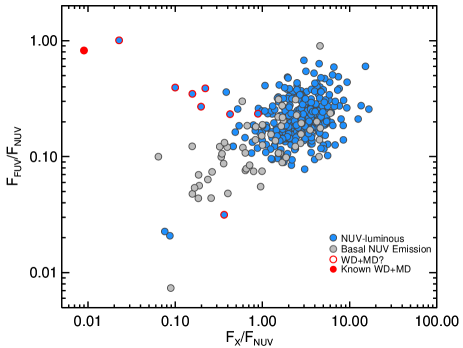
Figure 4.— The 387 NUV-detected early-M dwarfs in our sample that were also detected in GALEX FUV and ROSAT X-ray bands. Blue points correspond to NUV-luminous stars while gray points represent stars with basal NUV emission, as in Figure 3. Candidate and known WD+MD systems are shown by open and filled red circles, respectively.

3. FOLLOW-UP OBSERVATIONS

3.1. Medium-resolution Optical Spectra

We obtained medium-resolution ($\lambda/\Delta\lambda\sim 1000$) optical spectra for 2128 out of the 4805 M dwarfs in our sample. The majority of these (1307 spectra) were acquired using the Super-Nova Integral Field Spectrograph, SNIFS (Aldering et al. 2002; Lantz et al. 2004), mounted on the University of Hawaii 2.2-m telescope atop Maunakea. SNIFS uses a dichroic mirror to separate incoming light into blue (3200–5200Å) and red (5100–9700Å) spectrograph channels. We only used spectra from the red channel as M dwarfs have very low signal in the blue channel. All spectra had signal-to-noise ratios (${\rm SNR}$) $\gtrsim 80$ per resolution element in the red channel while avoiding the non-linear regime of the detector. Details of our SNIFS data reduction method can be found in Mann et al. (2012) and Lépine et al. (2013). SNIFS is an integral field spectrograph and therefore also provides limited spatial information in the form of image cubes. A SNIFS image cube covers 6 arcsec $\times$ 6 arcsec at 0.4 arcsec per pixel.

The remaining 821 spectra were obtained using four instruments on three different telescopes: the Mark III spectrograph and the Boller & Chivens CCD spectrograph (CCDS) on the 1.3-m McGraw-Hill telescope at the MDM Observatory on Kitt Peak (564 spectra); the RC spectrograph on the 1.9-m Radcliffe telescope at the South African Astronomical Observatory (SAAO) in South Africa (67 spectra); and the REOSC spectrograph on the 2.15-m Jorge Sahade telescope at the Complejo Astronómico El Leoncito Observatory (CASLEO) in Argentina (190 spectra). Details of the data reduction methods for these spectra are in Gaidos et al. (2014b).

3.2. Robo-AO High-resolution Imaging

We observed 193 M dwarfs in our sample with the Robo-AO laser adaptive optics and imaging system (Baranec et al. 2013; Baranec et al. 2014) mounted on the Palomar Observatory 1.5-m telescope. These observations were taken from 13 August 2013 to 25 May 2014 (UT). Robo-AO has a field of view of 44 arcsec $\times$ 44 arcsec at 43.10 mas per pixel. Typical PSF widths achieved at red-visible wavelengths are in the range of 0.12 to 0.15 arcsec and companions down to 6 magnitudes fainter than the primary can be detected (Law et al., 2014). We used a Sloan i’-band filter (York et al., 2000) for stars with $V<13$ and a long-pass filter cutting on at 600 nm (hereafter LP600) for fainter stars. Observations consisted of a sequence of full-frame-transfer detector readouts of the electron-multiplying CCD camera at the maximum rate of 8.6 Hz for a total of 90 sec of integration time. The individual images were corrected for detector bias and flat-fielding effects before being combined through post-facto shift-and-add processing that used the target as the tip-tilt reference star with 100% frame selection.

4. FALSE POSITIVES

The NUV-luminous M dwarfs in our sample (i.e., blue points in Figure 3 with spectral subtypes $\leq{\rm M3}$; see Sections 2.3 & 2.4) are presumably active due to their youth. However, early-M dwarfs can appear NUV-luminous for reasons other than stellar youth. These “false positive” (FP) systems include: single early-M dwarfs with unresolved background NUV sources within the $\sim$5 arcsec beam of GALEX; unresolved older binaries where one component is an early-M dwarf and the other component has persistent NUV emission (e.g., white dwarf or late-M dwarf); and short-period (${\rm P}<10$ days) tidally interacting binaries that induce ongoing activity in each other through spin-orbit synchronization.

We identified these FPs in our NUV-luminous sample using two approaches. First, we used literature searches (i.e., SIMBAD queries followed with checks in the literature) to identify known FPs (Section 4.1). Second, we identified new FP systems using four detection methods (described in Section 4.2 and summarized in Table 1) for which we also determined observational completenesses ($C$). We used the results of the second approach in a maximum likelihood scheme to estimate the overall FP rate in our NUV-luminous sample (Section 4.3). This allowed us to clean our sample of all identified FPs and then statistically correct the remaining sample for FPs when constructing the NUVLF (Section 5).

Table 1Methods for Detecting False Positives

Method	No. Obs.a	No. FPs b	Comp. (%)c
Robo-AO	193	26	94
H$\alpha$ Emission	562	37	100
H$\alpha$ Centroids	242	25	96
SuperWASP	312	15	83

4.1. SIMBAD Searches

We queried SIMBAD for our entire sample of NUV-luminous stars in order to identify any known FPs. We first searched for tight binaries including spectroscopic binaries (SBs), eclipsing binaries (EBs), and RS Canum Venaticorum (RS CVn) binaries. We followed up these candidates in the literature to confirm that they had orbital periods $<10$ days, at which point tidal interactions between companions likely result in synchronized orbits and therefore enhanced, persistent NUV emission beyond stellar youth (e.g., see Meibom et al. 2006 and references therein). We then searched for close binaries with separations $<5$ arcsec (i.e., unresolved by GALEX) and white dwarf or late-M secondary components, which also emit persistent NUV emission at older ages. We did not remove systems containing secondary M dwarf components with unknown spectral subtypes. We also searched for sources in our sample with background NUV objects within 5 arcsec, then inspected each of them individually to confirm that they were not double entries in the SIMBAD database.

We found 7 EBs, 7 RS CVn systems, and 8 SBs in our sample. We also found 18 close binaries with late-M or white dwarf components within 5 arcsec. There were 9 systems with background sources that were the probable source of NUV emission, rather than the M dwarf. These background FPs included a variety of sources: one contact EB, two SBs, one RS CVn star, two late-M dwarfs, one white dwarf, and two flare stars.

4.2. Detecting New False Positives

4.2.1 Robo-AO: Late-M Companions

We searched our 193 Robo-AO images (see Section 3.2) for close binaries whose secondary components may be causing FP NUV emission. We first searched for binaries using a principal component analysis (to flag elongated sources) and a Gaussian source finder (to flag multiple sources). We followed up these candidate binaries with manual (by-eye) checks to confirm the existence of clearly resolved binaries. We then developed a method that utilizes binary contrast ratios to identify systems where the secondary component is likely to be a late-M dwarf with elevated NUV emission (see Section 2.4).

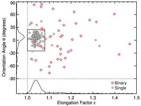
Figure 5.— Confirmed binaries (red diamonds) and single stars (gray circles) from our Robo-AO binary search. We used a principal component analysis to flag elongated sources outside the black box, and a Gaussian source finder to flag multiple sources inside the black box. These two methods were required to identify candidate binary systems due to the preferential elongation ($\varepsilon\sim 1.05$) and positive tilt ($\theta\sim 10^{\circ}$) seen in our dataset, as illustrated by the histograms. All candidate binaries were followed up with by-eye checks to confirm those as clearly resolved binaries for further analysis.

For the principal component analysis we calculated for each star an elongation factor, $\varepsilon$ (the ratio between the longer principal axis and the shorter principal axis), and an orientation angle, $\theta$ (the angle between the longer principal axis and the vertical image axis; the vertical axis of Robo-AO images is 23.9^∘ right of North). Only sources that were $>10\sigma$ above the noise were considered, and the noise was calculated using an outlier-resistant estimate of the dispersion in an area of empty sky around the source. In theory, single stars should have uniformly distributed $\theta$ with $\varepsilon=1$, while binary stars should also have uniformly distributed $\theta$ but $\varepsilon>1$ due to a companion skewing the otherwise symmetric distribution. However, Figure 5 illustrates that point sources in our dataset tend to have slight elongation ($\varepsilon\sim 1.05$) and positive tilt ($\theta\sim 10^{\circ}$). To account for this in the principal component analysis we ignored sources with these systematic effects (i.e., all stars inside the black box in Figure 5) and flagged all other sources as potential binaries due to their significant elongation. The Gaussian source finder was used to search the remaining parameter space (i.e., inside the black box in Figure 5) by looking for positive brightness perturbations that were $>3\sigma$ above the noise. We flagged all images with multiple positive brightness perturbations as potential binaries. We then used by-eye checks on all candidate binaries to identify only the clearly resolved systems for further analysis. These binaries and their calculated separations are listed in Table 2.

Despite the high resolution of Robo-AO, even the closest binaries resolved by this instrument are too far apart (i.e., several AU) to be tidally locked. However, Robo-AO can easily resolve binaries with separations $<5$ arcsec and thus unresolved with GALEX. Therefore contrast ratios derived from Robo-AO images can be used to identify the binaries in our sample with late-M secondary components likely causing FP activity. To identify such systems, we utilized the empirical relation between absolute Sloan i-band magnitude (M_i) and spectral subtype derived in Hawley et al. (2002). By calculating the difference between M_i at M3.5 and M_i at all other spectral subtypes, we derived the maximum allowable contrast ratio ($\Delta$m_lim) as a function of primary spectral subtype such that both components are early-M dwarfs. We confirmed that $\Delta$m_lim was applicable to images taken through either Robo-AO filter (Sloan i-band or LP600) by measuring the contrast ratios of a binary in our sample that was imaged in both bands; the difference in the measured contrast ratios was only $\sim$0.1 mags.

Table 2Robo-AO Binaries

Star	$\rho$ (arcsec)	$\sigma_{\rho}$ (arcsec)a	Contrast (mag)
PM_I00234+2418	2.20	0.01	3.13
PM_I00235+0947S	3.68	0.01	0.27
PM_I00235+2014	1.69	0.01	1.11
PM_I00505+2449S	1.00	0.01	0.81
PM_I00531+4829	1.26	0.01	1.59
PM_I00574+3736	4.58	0.02	5.36
PM_I01133+5855	2.07	0.01	3.44
PM_I01146+2057	1.42	0.01	2.12
PM_I01376+1835	1.69	0.01	0.09
PM_I01410+5308E	4.01	0.01	1.21
PM_I01480+4652	1.13	0.01	1.53
PM_I01491+0624	0.68	0.01	0.99
PM_I02024+1034	0.88	0.01	0.36
PM_I02208+3320	1.46	0.01	1.88
PM_I02347+1251	1.20	0.01	1.37
PM_I02408+4452	6.03	0.02	5.04
PM_I02560+1220	0.90	0.01	0.75
PM_I03053+2131	0.62	0.01	0.57
PM_I04284+1741	1.68	0.01	1.82
PM_I04310+3647	0.80	0.01	0.19
PM_I04333+2359	0.74	0.01	0.61
PM_I04453+1334	5.58	0.02	4.09
PM_I04499+2341E	2.39	0.01	0.83
PM_I04540+2200	3.85	0.02	3.81
PM_I05228+2016	3.61	0.01	1.78
PM_I05341+4732	2.47	0.01	1.01
PM_I06088+4257	1.25	0.01	0.75
PM_I06212+4414	1.37	0.02	3.18
PM_I06268+4202	0.85	0.01	1.25
PM_I11505+2903S	0.49	0.01	0.61
PM_I17038+3211	1.32	0.02	1.84
PM_I20514+3104	1.41	0.01	1.17
PM_I21010+2615	0.44	0.01	0.18
PM_I21221+2255	5.20	0.02	4.81
PM_I21410+3504	4.60	0.01	0.30
PM_I22006+2715	5.43	0.03	5.14
PM_I22234+3227	1.34	0.01	0.51
PM_I23045+4014	0.83	0.01	0.62
PM_I23063+1236	0.42	0.01	0.36
PM_I23300+1643	0.94	0.01	0.22
PM_I23318+1956W	5.40	0.01	1.75
PM_I23450+1458	1.17	0.01	0.27
PM_I23535+1206S	5.72	0.01	0.80
PM_I23578+3837	0.52	0.01	1.65

For each Robo-AO binary, we measured the contrast ratio by performing aperture photometry on each companion using the IRAF phot routine and a 20-pixel circular aperture. This aperture size was based on when the curve of growth for a typical single star reached an asymptotic value. Closer binaries required smaller aperture radii (5–15 pixels) to avoid contamination from companions. For sky subtraction we used median-combined, manually sampled patches of nearby empty sky around each system to ensure proper sky measurements. Figure 6 shows measured contrast ratios for all our Robo-AO binaries with separations $\lesssim 5$ arcsec. The black dashed line indicates our calculated $\Delta$m_lim as a function of primary spectral subtype. We found 26 binaries with primary spectral subtypes $\leq{\rm M3}$ but secondary components likely to be $>{\rm M3}$, making them potential FPs.

The observational completeness of our Robo-AO FP search was limited by two factors: (i) the maximum contrast ratio that Robo-AO can detect and (ii) the probability that a late-M companion was unresolved because its projected distance from the primary at the time of observation was too small. To estimate the completeness due to (i), we used the Cruz et al. (2007) $J$-band luminosity function, $n$(M_J), to calculate the number of M dwarf companions expected to have spectral subtypes $\geq{\rm M3.5}$ but earlier than the limit imposed by the maximum contrast ratio that Robo-AO can detect, $\Delta$m_max. We then compared that number to the total number of M dwarf companions expected to have spectral subtypes $\geq{\rm M3.5}$:

$$C=\frac{\sum_{i=1}^{binaries}\int_{\rm M_{\it J,3.5}}^{\rm M_{\it J,SpT_{i}}+\Delta m_{{\rm max},{\it i}}}n(\rm M_{\it J})dM_{\it J}}{\sum_{i=1}^{binaries}\int_{\rm M_{\it J,3.5}}^{M_{J,9.0}}n(\rm M_{\it J})dM_{\it J}}.$$ (2)

We adopted $\Delta$m${}_{\rm max}=6.0$, which is the maximum contrast ratio that Robo-AO can achieve at high “contrast-performance” (i.e., PSF sizes $>0.15$ arcsec) for separations $>1.0$ arcsec in the Sloan i-band (see Figure 5 in Law et al., 2014). The median PSF size and separation for the binaries in our Robo-AO sample were $\sim$0.17 arcsec and $\sim$1.41 arcsec, respectively, justifying this choice of $\Delta$m_max. We used relations from Hawley et al. (2002) to obtain $i-J$ color as a function of M_J, which allowed us to translate our Robo-AO contrast ratios from $i$- to $J$-band for use in Equation 2. We calculated each primary’s M_J using its $V-J$ color according to Equation 22 from Lépine et al. (2013). Evaluating Equation 2 gave a completeness factor of $\sim$0.97.

To estimate completeness due to (ii), we compared the median PSF size in our Robo-AO images ($\sim$0.17 arcsec) to the GALEX PSF size ($\sim$5.0 arcsec) and assumed a uniform source distribution on the sky (equivalent to an isotropic, uniform distribution of orbits with a log orbital period; Duquennoy & Mayor, 1991). This gave a $\sim$$3\%$ probability of an unresolved companion and thus a $\sim$0.97 completeness factor. The product the completenesses from (i) and (ii) gave a final observational completeness of $C\sim 0.94$ for our Robo-AO FP search.

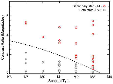
Figure 6.— Contrast ratios for systems identified by Robo-AO as having secondary components within 5 arcsec. The dashed line shows the maximum contrast ratio as a function of primary spectral subtype for systems where both stars are early-M dwarfs. Systems above the dashed line are predicted to have companions with spectral subtypes later than M3.

4.2.2 Optical Spectra: Missing H$\alpha$ Emission

Emission in the Balmer $\alpha$ line of hydrogen (H$\alpha$; $\lambda\approx 6563$Å) is another indicator of stellar activity and is strongly correlated with NUV emission (e.g., Lépine et al., 2013). FPs resulting from GALEX source confusion can therefore potentially be identified by the absence of H$\alpha$ emission despite significant amounts of NUV emission (i.e., NUV emission at least $2.5\sigma$ above the basal level; see Section 2.3). This is because sources that are unresolved by GALEX’s $\sim$5 arcsec beam can be resolved by spectroscopy with $\sim$1 arcsec resolution. We therefore computed H$\alpha$ equivalent widths (EW_Hα) for the 2128 stars in our sample with medium-resolution optical spectra (see Section 3.1).

To calculate EW_Hα we first shifted each spectrum to its rest frame by applying wavelength offsets found by matching our observed spectra to PHOENIX model atmospheres. We used the BT-SETTL version of the PHOENIX atmospheric model code (Allard et al. 2013; Rajpurohit et al. 2013) with the CIFIST grid and Caffau et al. (2011) abundances for the Sun. Following Lépine et al. (2013), we measured the flux within a 14Å-wide spectral region (6557.61–6571.61Å, in air) relative to pseudo-continuum regions (6500–6550Å and 6575–6625Å, in air). Errors were calculated using a Monte Carlo method that assumed Gaussian-distributed noise and random wavelength calibration errors of 0.5Å. As noted by Lépine et al. (2013), this choice of continuum region systematically underestimates EW_Hα values due to differences between our pseudo-continuum and the true spectral continuum. We therefore applied a small offset (0.3Å) so that stars with basal NUV emission had a mean EW${}_{\rm H\alpha}\approx 0$. This did not affect our FP analysis as the offset was applied to the entire population.

Figure 7 shows our measured EW_Hα values as a function of our selection cutoff for NUV-luminous stars (see Section 2.3). As expected, the stars with basal NUV emission (gray points, corresponding to those in Figure 3) are located in a band with negligible EW_Hα. The NUV-luminous stars (blue points, corresponding to those in Figure 3) form a distinct locus where increasing NUV emission corresponds to increasing EW_Hα values. However, a subset of NUV-luminous stars have lower-than-expected EW_Hα values (i.e., they lie significantly below the NUV-luminous locus) and are presumably FPs due to GALEX source confusion. We fit a line to median values of EW_Hα vs. relative NUV emission for the NUV-luminous population (black dashed line in Figure 7) to determine the expected EW_Hα value for a young M dwarf with a given NUV emission level. We identified 37 stars with EW_Hα values more than $3\sigma$ below the expected value, making them likely FPs.

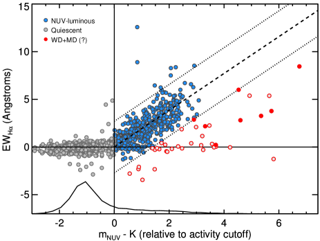
Figure 7.— EW_Hα as a function of our selection cutoff for NUV-luminous stars (see Section 2.3). Blue and gray points are the same as in Figure 3. The dashed black line is the median fit to the NUV-luminous population, representing the expected EW_Hα of a young M dwarf with a given NUV emission level; 3$\sigma$ boundaries are shown by dotted black lines. Suspect FPs, outlined in red, reside at least 3$\sigma$ below their expected EW_Hα value. Filled red circles indicate known or candidate WD+MD systems (see Section 2.6).

Interestingly, all known WD+MD binaries in our sample as well as the new candidate WD+MD systems identified in this work (see Section 2.6) were flagged as FPs using this detection method. As shown in Figure 7, these WD+MD pairs have anomalously high NUV emission relative to their EW_Hα values, as expected (see Section 2.6). It is also important to note the distinct lack of stars with high EW_Hα values but basal NUV emission levels (upper left quadrant in Figure 7); because the NUV and H$\alpha$ measurements were taken at different epochs, this may illustrate consistent levels of activity for the vast majority of stars in our sample. This would suggest that our sample contains very few flare stars and thus a low probability of misidentified FPs due to stellar variability. Of course the same reasoning could be applied to the significant population of sources with high NUV emission but low EW_Hα values to argue for evidence of flaring; however, as discussed above, this population also contains FPs, which complicates the interpretation.

We estimated the observational completeness for this FP detection method using an injection and recovery method. We replaced the region of H$\alpha$ emission in each star’s spectrum with the median of the surrounding continuum flux, then injected a synthetic H$\alpha$ signal with an equivalent width equal to the expected value for that star’s NUV emission level (using the black dashed line in Figure 7 as a guide). We also added random Gaussian noise scaled to the noise in the surrounding continuum regions. We re-measured the EW_Hα values using the same method as above, repeating 100 times and taking the average of the resulting equivalent widths for each star. We then checked whether this EW_Hα value was within 3$\sigma$ of the expected value. In all cases the signal was recovered, implying $C\sim 1.0$ for our EW_Hα FP detection method.

4.2.3 SNIFS Integral Field Spectra: H$\alpha$-emitting Companions

SNIFS image cubes provide both spatial and wavelength dimensions that can be used in conjunction to search for FPs. In particular, they can be used to find binary systems appearing young due to unresolved late-M companions with persistent activity despite being old. In such cases, the early-M primary exhibits basal NUV emission but dominates the continuum signal (making the system appear as a single early-M dwarf), while the unresolved late-M companion is the source of the stronger H$\alpha$ emission and presumably also the NUV flux. This configuration is detectable as a shift between the centroid of a white-light image versus the centroid of an H$\alpha$ image. We used this method of detecting FPs in addition to our Robo-AO image analysis (Section 4.2.1) because H$\alpha$ traces activity and we have more SNIFS image cubes than Robo-AO images.

We performed this analysis on the 242 stars in our NUV-luminous sample with SNIFS image cubes. To create the white-light image we summed the SNIFS image cube over all wavelengths covered by the spectrum. We identified the source centroid location by employing a principal component analysis using only points that were $>10\sigma$ above the noise. The noise was calculated using an outlier-resistant estimate of the dispersion around the outer edge of the image; we used the outer edge due to the small size of SNIFS images (14 pixels$\times$14 pixels). To create the H$\alpha$ image we summed the SNIFS image cube across only wavelengths covering the H$\alpha$ spectral line (see Section 4.2.2 for our H$\alpha$ line parameters), then subtracted the continuum and divided by the noise. The continuum was estimated using the median value of surrounding wavelength regions multiplied by the number of wavelength elements covered by the spectral line, and the noise was found by taking the standard deviation of the continuum regions. To identify the H$\alpha$ centroid location, we again used a principal component analysis but first applied a mask to consider only pixels that were also used to calculate the white-light centroid. We discarded systems lacking any significant H$\alpha$ emission.

Figure 8 shows the distribution of offsets between the white-light and H$\alpha$ centroids. We fit a Rayleigh function to the distribution using the IDL routine mpfit (Markwardt, 2009), which returned a mean offset of $\mu\approx 0.37$ pixels and a dispersion of $\sigma\approx 0.20$ pixels. We flagged systems with centroid offsets $>3\sigma$ above the mean as potential FPs, then used by-eye checks to confirm 25 systems with clear shifts in their image centroids. We estimated the observational completeness as the ratio of the area over which false positives could be detected (i.e. the area of the annulus from $r=3\sigma$ to $r=r_{max}$, where $r_{max}$ is the maximum centroid offset in our sample) to the total survey area (i.e., the area of a circle with $r=r_{max}$). This resulted in an observational completeness of $C\sim 0.96$ for our centroid offset detection method.

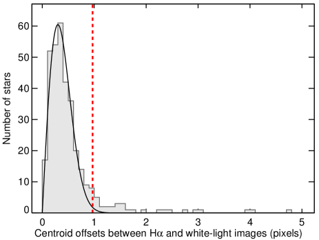
Figure 8.— Centroid offsets between white-light and H$\alpha$ images for the 242 NUV-luminous sources in our sample with SNIFS image cubes. A Rayleigh fit to the distribution (black solid line) produced a mean of $\mu=0.37$ and error of $\sigma=0.20$. Systems with offsets $>3\sigma$ above the mean (red dashed line) were flagged as potential FPs then followed up with by-eye checks to confirm the likely existence of an unresolved late-M companion.

4.2.4 SuperWASP Light Curves: Tidally-Locked Binaries

Time-series photometry from the SuperWASP exoplanet survey (Pollacco et al., 2006) can be repurposed to identify very short-period, interacting stellar binaries (e.g., Norton et al., 2011). These systems of tidally-locked, synchronously rotating stars remain magnetically active and rapidly rotating due to the transfer of angular momentum from their orbits to their spins. They exhibit photometric variability because of transits and/or fixed patterns of spots established by the interacting magnetic fields of the companions. Even though a young, single M dwarf can also have a surplus of star spots due to elevated activity, these spots tend to be uniformly distributed across the surface, which likely dampens any induced light curve variability (see Barnes et al., 2011, and references therein). Moreover spots on single stars tend to migrate, causing the phases of their light curve signals to change over time.

We therefore cross-referenced our NUV-luminous sample with the SuperWASP database, which is available online. We used a 3 arcsec search radius and only considered light curves with more than 1,000 data points due to the limited photometric precision of SuperWASP. This resulted in a sample of 312 NUV-luminous sources with SuperWASP light curves. We inspected each of these light curves for stellar variability by computing their Lomb-Scargle periodogram (Scargle, 1987), which estimates a frequency spectrum based on a least-squares fit to sinusoids. We only considered signals with a false-alarm probability of $<0.1$%. We ignored periods within 2% of one day and fractions thereof (1/4, 1/3, 1/5, etc.) as those are likely artifacts due to observing schedules (Gaidos et al., 2014a). We used a stricter 10% filter around periods with stronger systematics (0.5, 1.0, 1.5, and 2.0 days).

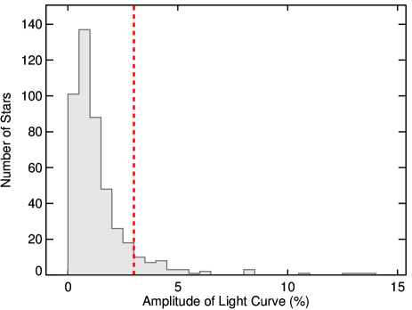
Figure 9.— Amplitudes of all SuperWASP light curves available for our NUV-luminous sources. The dashed line shows the amplitude cutoff above which sources were considered candidate tidally interacting binaries (if they also fulfilled our period criteria; see Section 4.2.4).

To identify candidate tidally interacting binaries we selected light curves that featured large amplitude variations ($>2.6$%) at short periods ($<10$ days) with phases that appeared perfectly Keplerian (i.e., stable over many cycles). The period criterion was based on the orbital period at which tidal interactions between companions begin to synchronize orbits and therefore enhance stellar activity (see Meibom et al., 2006, and references therein). The amplitude criterion was obtained from running the Lomb-Scargle periodogram on all known eclipsing binaries in LG11 with SuperWASP light curves, then taking the minimum amplitude recovered as our lower limit.

Figure 9 shows this limit in the context of all SuperWASP light curve amplitudes derived from our sample. From the preliminary list of candidate FPs generated by applying the above criteria, we used by-eye checks to identify 15 light curves with clear sinusoidal signals consistent with those of known tidally locked binaries. We then divided each of these light curves into halves and re-ran the analysis on both sections to check that the period remain unchanged, indicating variability due to regular eclipses rather than varying star spot patterns.

We estimated observational completeness using a method of injection and recovery of artificial sinusoidal signals. We randomly selected 100 SuperWASP light curves from our sample and randomized the fluxes of the data points. We then injected signals with randomly selected periods of 0.1–10 days (i.e., our FP period search criteria) and amplitudes of 2.6–6.7% (i.e., our FP amplitude search criteria limited by the maximum amplitude found in our sample). We then re-performed our Lomb-Scargle periodogram search, using the same period filters and false-alarm probability as before, to test whether we would have recovered the injected signals as candidate FPs. This produced an observational completeness of $C\sim 0.83$ for our SuperWASP FP detection method.

4.3. Derivation of an Overall False Positive Rate

Construction of an accurate NUVLF requires the identification and consideration of FPs, i.e. systems that appear NUV-luminous for reasons other than stellar youth. Our approach was to (i) estimate the overall FP rate among our NUV-luminous sample based on FP detection methods for which we could determine observational completenesses (Section 4.2); (ii) remove FPs identified using these FP detection methods as well as known FPs from the literature (Section 4.1); and then (iii) use our derived overall FP rate to statistically correct the remaining NUV-luminous stars in our sample not yet flagged as FPs (Section 5.2). The last step was necessary to account for the fact that not all NUV-luminous sources were observed with all FP detection methods, and also because our FP detection methods cannot each detect all possible types of FPs (e.g., the Robo-AO method cannot resolve tidally locked binaries).

We used a maximum likelihood approach to estimate the overall FP rate in our NUV-luminous sample. When screening a source with our FP detection methods in Section 4.2, the source is either identified as a FP or it is not. We can describe the likelihood of these two possible outcomes, $f(p)$ and $g(p$), respectively, in terms of the overall FP rate ($p$) and the completenesses of the different FP detection methods that were applied to the source ($C_{j}$):

$$g(p)=(1-p)+p\prod_{j}^{missed}(1-C_{j})$$ (3)

and

$$f(p)=p\big{[}1-\prod_{j}^{missed}(1-C_{j})\big{]}.$$ (4)

Equation 3 is the probability that a source was not identified as a FP: the first term is the probability that the source was not a FP, while the second term is the probability that the source was a FP but that it was missed by all the FP detection methods that were applied to it. Equation 4 is the probability that a source was identified as a FP: the term in the brackets is the probability that the source was identified as a FP by the detection methods that were applied to it, and this term is then multiplied by the actual false-positive rate. This approach assumes that there are no “false negatives” (i.e., it assumes that our FP detect methods cannot wrongly classify a source as a FP). It also assumes that a source is a FP if just one of our methods detected it as a FP. We found the value of $p$ that maximizes the likelihood:

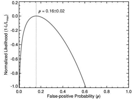
Figure 10.— The maximum likelihood (see Equation 5) used to determine the most probable value of the overall FP rate, $p$, in our NUV-luminous sample of early-M dwarfs.

$$\ln\mathscr{L}=N_{\rm FP}\ln p+\sum_{k}^{\rm NFP}\ln\big{[}1-p\big{(}1-\prod_{m}(1-C_{m})\big{)}\big{]},$$ (5)

where $N_{\rm FP}$ is the total number of FPs found using our FP detection methods, and $C_{m}$ is the observational completeness of each FP detection method applied to a given star that was not found to be a FP (NFP). Solutions to Equation 5 for all possible values of $p$ are shown in Figure 10, indicating a most likely FP rate of $p\sim 0.16\pm 0.02$. We estimated the errors by fitting an inverted parabola around the peak in the log likelihood, then using the uncertainty on the curvature of the fit (i.e., $\sigma_{x}=1/\sqrt{-2c}$ for a parabola described by $y=a+bx+cx^{2}$).

5. THE NUV LUMINOSITY FUNCTION

5.1. Fractional NUV Luminosity

We defined a fractional NUV luminosity to describe the distribution of NUV luminosities with respect to a basal value:

$$R^{\prime}_{\rm NUV}=\frac{\rm L_{\rm NUV}-\rm L_{\rm basal}}{\rm L_{bol}},$$ (6)

where L_NUV is the total NUV luminosity, L_basal is the basal NUV luminosity, and L_bol is the bolometric luminosity. To obtain these parameters from the observed quantities shown in Figure 3, we re-arranged the color relation $m_{\rm NUV}-K_{\rm S}=M_{\rm NUV}-{\rm M}_{K_{\rm S}}$ to obtain an expression for absolute NUV magnitude: ${\rm M}_{\rm NUV}={\rm M}_{K_{\rm S}}+(m_{\rm NUV}-K_{\rm S})$. We calculated M${}_{K_{\rm S}}$ by translating $V-J$ color into M_J using Equation 22 from Lépine et al. (2013) then converting M_J to M${}_{K_{\rm S}}$ using $J-K_{\rm S}=0.854$ ($J-K_{\rm S}$ color varies little for early-M dwarfs; here we used the median of our sample). To translate M_NUV into L_NUV we used the GALEX zero points to convert magnitude into flux density (ergs^-1 s^-1 cm^-2 Å^-1) then multiplied by the effective GALEX NUV bandwidth ($\Delta\lambda=732$ Å) to get the NUV flux, F_NUV. We then input F_NUV into L${}_{\rm NUV}=4\pi d^{2}\rm F_{\rm NUV}$ where $d=10$ pc (in accordance with the definition of absolute magnitude). We also applied this method to the median fit shown in Figure 3 (black dashed line) to obtain L_base as a function of $V-J$ color. To calculate L_bol we used the standard equation L${}_{\rm bol}={\rm L}_{\odot}\times 10^{-0.4({\rm M}_{bol}-{\rm M}_{bol,\odot})}$ where M${}_{bol,\odot}=4.7554$ magnitudes and L${}_{\odot}=3.8270\times 10^{33}$ ergs^-1 s^-1 (Mamajek, 2012). To obtain ${\rm M}_{\rm bol}$ we used the $K_{\rm S}$ bolometric correction from Leggett et al. (2001).

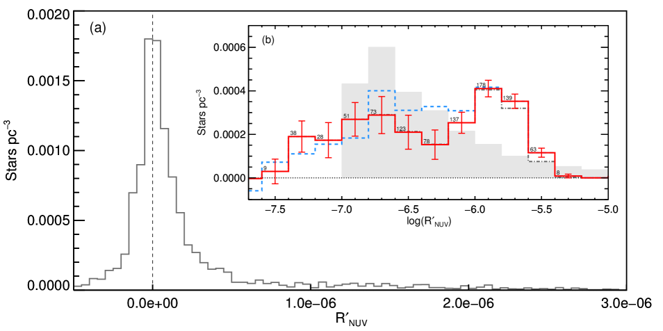
Figure 11.— (a) Our derived NUVLF for young, early-M dwarfs using the $1/V_{max}$ method described in Section 5.2. The peak centered on zero consists of stars exhibiting basal NUV emission and the extended tail (only partially shown here) consists of NUV-luminous stars that are presumably young/active. (b) The residual NUVLF, now shown in log space, representing only the young early-M dwarfs. The residual distribution in (b) was found by subtracting opposing sides of the distribution in (a). The red solid line shows the NUVLF when including upper limits (see Section 5.3), while the blue dashed line shows the NUVLF when ignoring upper limits (see Section 5.2). For the residual distribution that includes upper limits, the number of stars in each bin is shown for reference and error bars were found using bootstrap sampling. The gray dash-dotted line (mostly coincident with the red solid line except at the highest $R^{\prime}_{\rm NUV}$ values) shows the NUVLF derived using a varying FP rate (see Section 6.1). The light gray filled histogram is the best-fit model assuming a constant star-formation rate and an age-activity relation described by a two-parameter power law (see Section 6.2).

5.2. The $1/V_{\rm max}$ Method

The “$1/V_{\rm max}$” method (Schmidt, 1968) is used to construct luminosity functions by accounting for the bias of flux-limited surveys toward intrinsically bright sources. This is done by inversely weighting sources by the volume of space over which they could have been detected by the survey. Thus bright sources are assigned smaller weights to correct for being detectable to larger distances. The luminosity function is then calculated by summing the weights (rather than number of stars) in each luminosity bin, giving units of stars pc^-3.

To apply the $1/V_{\rm max}$ method to our sample, we calculated for each star the maximum distance at which it would have been included in LG11 and also detected by GALEX. Thus the limiting detection distance of each star was determined by one of three factors: (i) the $J$-band magnitude limit ($J<10$) of the LG11 catalog; (ii) the proper motion limit ($\gtrsim 40$ mas in the north, $\gtrsim 100$ mas in the south) of the LG11 catalog; and (iii) the GALEX sensitivity limit. Because GALEX sensitivity varies across the sky due to varying tile exposure times, we estimated the limiting NUV magnitude for each star in our sample (see Section 5.3) to create a map of limiting NUV magnitude across the sky. Then for each star we compared its two LG11 limiting detection distances to each GALEX limiting detection distance across the sky, recording the smallest value in each case. The average of the cube of these smallest detection distances was then used to calculate $V_{\rm max}$ for that star. The star’s contribution to the NUVLF was then determined by its weight, $1/V_{\rm max}$.

To account for FPs, we first removed all FPs found in the literature (Section 4.1) or with our FP detection methods (Section 4.2). We then statistically accounted for FPs in the remaining stars by multiplying their $1/V_{\rm max}$ weights by $1-p$ (i.e., the probability of not being a FP). For NUV-luminous stars we used $p=0.16$ (see Section 4.3) and for all other stars we used $p=0$. There were also 92 sources in our sample with limiting detection distances that were found to be smaller than their actual distance. This was mostly due to anomalies in survey sensitivities (e.g., 67 of these sources had declinations $<-20^{\circ}$ where LG11 proper motion limits can vary). We removed these sources from our sample before constructing the NUVLF, however only 9 of these sources were members of our NUV-luminous sample (these are flagged in Table 4).

The resulting NUVLF is shown in the main panel of Figure 11. By construction, the peak at $R^{\prime}_{\rm NUV}\approx 0$ consists of stars with basal levels of NUV emission (designated by gray points in Figure 3) while the extended tail toward higher $R^{\prime}_{\rm NUV}$ values consists of the NUV-luminous stars (designated by blue points in Figure 3). The negative values in the distribution result from the subtraction of a median-fit basal level when calculating $R^{\prime}_{\rm NUV}$ (see Equation 6). We applied a small offset ($R^{\prime}_{\rm NUV}\sim 1.5\times 10^{-8}$) to shift the distribution peak to zero. This was essentially a correction to our median basal fit (black dashed line in Figure 3), which was likely skewed to higher $R^{\prime}_{\rm NUV}$ values because (i) we were not considering upper limits and (ii) we were only considering stars with the lowest NUV flux errors, which typically have the highest NUV fluxes.

The shape of the peak in the main panel of Figure 11 is dictated by photometry errors and the intrinsic width of the basal NUV locus (see Section 2.5). We needed to extract the extended tail of NUV-luminous stars for our analysis of the NUVLF of young early-M dwarfs. We did this by reflecting the negative side of the distribution about the ordinate and subtracting it from the positive side of the distribution. This essentially removed the population of stars with basal NUV emission from the distribution. This assumes that the distribution of $R^{\prime}_{\rm NUV}$ values in the basal population is symmetric about zero, but does not assume any distribution in particular. The median GALEX counts for basal NUV sources ($\sim$50 counts) were sufficiently high that the distribution due to GALEX Poisson errors should be fairly symmetric.

This extraction process gave a residual distribution that represents the NUVLF of young early-M dwarfs, shown as the blue dashed line in the inset of Figure 11 and tabulated in Table 3. Errors were found using a standard bootstrap method. We sampled with replacement from the original set of $R^{\prime}_{\rm NUV}$ values until we obtained a bootstrap sample that contained the same number of data points as the original sample. We then re-constructed the NUVLF following the same steps as above, but instead using the bootstrap sample. We repeated this 100 times and used the standard deviation in each bin as an estimate of our errors.

5.3. Including Upper Limits

Most of the LG11 stars without matches in the GALEX AIS catalog (2226 out of 3622) are either late-M dwarfs (and therefore not considered in this study) or stars within 20 degrees of the Galactic plane (where GALEX AIS coverage is sparse; Bianchi et al. 2014). To determine which of the remaining 1396 LG11 stars were true non-detections (i.e., stars located in an area of sky observed by GALEX AIS but too faint to be detected), we searched for GALEX AIS tiles covering their coordinates using the aforementioned GalexView online tool (see Section 2.1). We only considered GALEX AIS tiles with centers less than 0.5 degrees from the LG11 coordinates of the candidate non-detections. This separation limit ensured that the stars would have actually been located on the tile, but not on the tile edge where photometry can be significantly degraded (Bianchi et al., 2014). This search resulted in the identification of 638 non-detections for which we estimated upper limits.

To calculate upper limits, we derived a relation between GALEX exposure time ($t_{\rm NUV}$) and limiting NUV magnitude ($m_{\rm lim}$) using the online GALEX Exposure Time Calculator. We queried the tool for exposure times given various $m_{\rm NUV}$ values and required ${\rm SNR}\sim 2$. We used a hypothetical star with ${\rm T_{\it eff}}=3500$ K and coordinates $\alpha=240^{\circ}$ and $\delta=-11^{\circ}$ (i.e., an early-M dwarf with median LG11 declination and located away from the Galactic plane). To check the relation, we plotted $m_{\rm NUV}$ vs. $t_{\rm NUV}$ for the 5267 GALEX-detected LG11 stars; as expected, the derived relation between $t_{\rm NUV}$ and $m_{\rm lim}$ corresponded to the lower (NUV-dim) bound of the NUV-detected population. We obtained $m_{\rm lim}$ values for the 638 non-detections by using the $t_{\rm NUV}$ values of their associated GALEX AIS tiles with our derived relation.

We considered these upper limits in our NUVLF using the method of Avni et al. (1980). This method employs a non-parametric, recursive approach to statistically account for upper limits when constructing a luminosity function (see Equation 6 in Avni et al., 1980). As before, we replaced the number of stars in each $R^{\prime}_{\rm NUV}$ bin with the sum of their $1/V_{\rm max}$ weights in order to account for survey biases toward brighter stars. However, because we were considering GALEX upper limits with this method, we relaxed any GALEX constraints on $V_{\rm max}$ by only considering the detection distance limits imposed by LG11 when calculating $V_{\rm max}$. We again had to apply a small offset ($R^{\prime}_{\rm NUV}\sim 6.5\times 10^{-9}$) to shift the distribution peak to zero; this correction was much smaller than before, most likely because we are now taking into account upper limits. The resulting NUVLF is shown as the red line in the insert of Figure 11 and tabulated in Table 3 with errors calculated using the same bootstrap method described in Section 5.2.

Table 3Near-Ultraviolet Luminosity Functions

$\log(R^{\prime})$	$\rho_{V_{max}}$a	$\rho_{\rm Avni}$b
	($10^{-5}$ stars pc-3 dex-1)	($10^{-5}$ stars pc-3 dex-1)
-7.50	36.1 $\pm$ 41.6	14.8 $\pm$ 28.4
-7.30	55.1 $\pm$ 52.0	94.9 $\pm$ 35.9
-7.10	77.3 $\pm$ 78.7	86.6 $\pm$ 40.3
-6.90	91.6 $\pm$ 74.9	134.6 $\pm$ 38.6
-6.70	200.1 $\pm$ 65.6	144.2 $\pm$ 42.6
-6.50	155.2 $\pm$ 58.8	104.9 $\pm$ 39.0
-6.30	163.9 $\pm$ 52.1	76.3 $\pm$ 33.7
-6.10	154.4 $\pm$ 37.5	126.6 $\pm$ 24.3
-5.90	208.3 $\pm$ 33.3	205.1 $\pm$ 19.1
-5.70	176.1 $\pm$ 27.5	176.1 $\pm$ 16.5
-5.50	57.9 $\pm$ 21.4	57.9 $\pm$ 10.3

6. DISCUSSION

6.1. Uncertainties and Sensitivities

The two principal uncertainties in our derivation of the NUVLF are: (i) the overall FP rate, $p$, which we used to statistically correct for FPs when constructing the NUVLF (Section  4.3); and (ii) the distances used to compute the limiting detection volumes, $V_{max}$, which we used to weight each star’s contribution to the NUVLF (Section  5.2). We address these two issues below.

Our derived overall FP rate of $p\sim 16$% is consistent with the $\sim$16% spectroscopic binary rate among nearby X-ray luminous M dwarfs found by Shkolnik et al. (2009). One might expect our FP rate to be higher as our definition of a FP encompasses additional, wider binaries. However Shkolnik et al. (2009) selected their sample based on X-ray fluxes from the ROSAT All Sky Survey, which was less sensitive to active stars than the GALEX AIS. Thus their sample was more biased toward the most active objects, which likely have higher FP rates (see below). Agreement between our FP rate and that of Shkolnik et al. (2009) may therefore simply be a coincidence resulting from several factors.

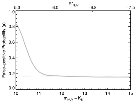
Figure 12.— Varying FP rate among our NUV-luminous sample as a function of $m_{\rm NUV}-K_{\rm S}$ and $R^{\prime}_{\rm NUV}$. The FP rate remains constant at $\sim$16% (i.e., the overall FP rate found in Section 4.3) until $m_{\rm NUV}-K_{\rm S}\sim 11$, then rises to $>80$% when considering only the most NUV-luminous M dwarfs.

The NUV luminosities in our sample span several dex (see Figure 11). Thus a single, overall FP rate may be insufficient to describe the entire population, as the most NUV-luminous sources may have significantly higher FP rates. We tested this by progressively removing the dimmest NUV sources from our sample, then repeating the maximum likelihood estimation in Section 4.3 to re-derive $p$ based on the cropped sample. Results are given in Figure 12, which shows a constant FP rate of $p\sim 16$% (i.e., our overall FP rate) until $m_{\rm NUV}-K_{\rm S}\sim 11$. At higher NUV luminosities, the FP rate steadily increases, reaching $p\sim 80$% by $m_{\rm NUV}-K_{\rm S}\sim 10$. To test the implications of this result, we re-derived our NUVLF using this varying FP rate (instead of the constant $p\sim 16$% value) when multiplying the $1/V_{\rm max}$ weights by $1-p$ to statistically account for FPs (see Section 5.2). We did not expect significant changes to the NUVLF, as there are few stars in our sample with high enough NUV luminosities to require FP rates that are significantly larger than the overall FP rate. The results are compared to the original NUVLF in the inset of Figure 11. The consistency between the two NUVLFs suggests that our derivation is not particularly sensitive to this varying FP rate. Still, our use of a single FP rate is a gross simplification of reality where there are multiple, sometimes unrelated sources of FPs, each of which cannot be detected by all our methods applied in Section 4.2. A more rigorous approach would use a modified version of Equation 5 to estimate multiple $p$ values, one for each FP source, and also account for the completenesses of each method for each FP source. However the outcome of the sensitivity analysis described above suggests that our results would not change significantly.

Another source of uncertainty in our derivation of the NUVLF is our estimation of stellar distances, which we used to calculate $V_{max}$ and thus the weighted contribution of each star to the NUVLF. For most sources we used a $J$-band photometric distance, where M_J was estimated from $V-J$ color using Equation 22 in Lépine et al. (2013). However we substituted more accurate parallax distances for the 561 stars in our sample that also had trigonometric parallax measurement with errors $<10$%. We used the average difference between these photometric and parallax distances to estimate fractional errors as a function of stellar distance. These ranged from $\sim$50% for distances of $\sim$3 pc (the minimum distance in our sample) to $\sim$10% for distances of $\sim$40 pc (the distance containing 95% of our sample). We then tested how these distance uncertainties impacted our derived NUVLF using a Monte Carlo approach. We perturbed each distance by a random Gaussian deviate scaled to our estimated fractional errors, then re-ran our derivation of the NUVLF. We repeated this 100 times and took the standard deviation in each luminosity bin as an estimate of the impact of our distance uncertainties on our NUVLF. The impact appeared to be negligible: the variation was only $\sim$14% of the original NUVLF in each bin, well within the errors estimated by bootstrap sampling (see Section 5.2).

6.2. NUV Age-Activity Relation

Relations between stellar age and emission at high-energy wavelengths are typically expressed as two-parameter power laws of the form F${}_{\lambda}=\alpha t^{\beta}$ (c.f., Ribas et al., 2005) where $t$ is the age of the star and the two parameters, $\alpha$ and $\beta$, are the zero point and slope of the power law, respectively. Stelzer et al. (2013) derived an age-activity relation for early-M dwarfs by combing their sample of 159 nearby field M dwarfs (assuming an age of $\sim$3 Gyr) with an additional sample of young ($\sim$1 Myr) M dwarfs from the TW Hya association. They found that $\beta=-0.84\pm 0.08$ at GALEX NUV wavelengths.

Because stellar ages for our sample are mostly unknown, we first attempted to infer an age-activity relation by fitting our observed NUVLF to model NUVLFs constructed from assumed power-law age-activity relations. To create model populations, we assumed a constant star-formation rate (and thus a uniform age distribution) with a maximum age of $\sim$10 Gyr (i.e., the approximate age of the Galactic disk at the present solar radius; Bergemann et al., 2014). We then used a two-parameter power law, described above, to assign $R^{\prime}_{\rm NUV}$ values to each synthetic star based on its model age. We created the model NUVLF by binning the synthetic population according to the same $R^{\prime}_{\rm NUV}$ bins as in the inset of Figure 11, then normalizing the model distribution such that the integral under the model function equaled that of the real function. We searched for best-fit parameters by minimizing reduced $\chi^{2}$. We calculated reduced $\chi^{2}$ by taking the difference between the model and observed NUVLFs at each $R^{\prime}_{\rm NUV}$ bin, applying the errors shown in the inset of Figure 11 to the observations, and dividing by the number of bins minus the number of power-law parameters. We found best-fit parameters of $\beta\approx-1.29$ and $\alpha\approx 2.4\times 10^{-6}$ with reduced $\chi^{2}\approx 6.3$. The best-fit model is compared to the observed NUVLF in the inset of Figure 11. Clearly this simplified model is unable to account for the observed NUVLF, likely due to our two key assumptions: (i) our neglect of a constant (i.e., saturated) level of NUV emission at very young ages and/or (ii) our assumption of a constant star-formation rate. We discuss (i) below and (ii) in Section 6.3.

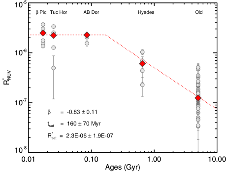
Figure 13.— Photosphere-subtracted fractional NUV luminosity, $R^{*}_{\rm NUV}$, as a function of age for the 20 YMG members in our sample as well as 28 old field stars identified by their high space motions. Red diamonds are median $R^{*}_{\rm NUV}$ values for each age group. The best-fit broken power law, shown by the dotted red line with parameters printed for reference, was found using $\chi^{2}$ minimization and bootstrap sampling (see text for details).

Saturated (i.e., constant) NUV emission in young early-M dwarfs was recently reported by Shkolnik & Barman (2014). They used early-M members of nearby young moving groups (YMGs) to derive a NUV age-activity relation that showed NUV emission remaining constant for $\approx 300$ Myr then declining as a power law with $\beta=-0.84\pm 0.09$. This power law index agrees with the previous findings of Stelzer et al. (2013), who did not consider saturated NUV emission due to the lack of stars younger than a few hundred Myr in their sample. We therefore used the YMG members in our sample to empirically derive a power-law age-activity relation that included a saturation component. We first searched the literature to identify 32 candidate YMG members in our sample. We then required high ($\geq 95$%) membership probabilities, which we obtained using the BANYAN (Bayesian Analysis for Nearby Young AssociatioNs; Malo et al., 2013) online tool. For the Hyades, which is not included in BANYAN, we used the approach of Shkolnik & Barman (2014) by requiring a kinematic link to the YMG. We also removed any FPs identified in Section 4. This resulted in a final set of 20 YMG members, which are flagged in Table 4.

In order to extend our age-activity relation to older field stars, as well as make our derived age-activity relation comparable to previous works, we re-defined our fractional NUV luminosity ($R^{\prime}_{\rm NUV}$; see Equation 6). Instead of subtracting the observed basal NUV luminosity (L_basal) we subtracted the photospheric NUV luminosity predicted by PHOENIX models (L_phot) to obtain $R^{*}_{\rm NUV}$ (the predicted values of L_phot as a function of $V-J$ are shown by the dash-dotted line in Figure 3). The $R^{*}_{\rm NUV}$ values for our 20 YMG members are plotted as a function of their age in Figure 13. Also shown are 28 older field stars from our sample, which were identified by having space motions $>1\sigma$ from the mean of active/young stars in at least two spatial dimensions (space motion information was obtained from Lépine et al., 2013). Similar to the findings of Shkolnik & Barman (2014), we observed a saturated level of NUV emission lasting a couple Myr, followed by a power-law decline.

To derive our age-activity relation, we fit a broken power law to the median $R^{*}_{\rm NUV}$ values of each age group. To obtain the best-fit parameters and associated errors, we constructed 100 bootstrap samples from our data, found the model parameters associated with the minimum reduced $\chi^{2}$ for each bootstrap sample, then took the mean and standard deviation. The results are shown in Figure 13, indicating a saturated NUV emission level at $R^{*}_{\rm NUV}=2.3\pm 0.19\times 10^{-6}$ until $160\pm 70$ Myr of age, after which NUV emission declines as a power law with slope $\beta=-0.83\pm 0.11$. Our $\beta$ value agrees well with those found by Stelzer et al. (2013) and Shkolnik & Barman (2014). Our saturation timescale is also consistent with that of Shkolnik & Barman (2014), although their value of 300 Myr is slightly higher, possibly due to our lack of data points between 100 and 600 Myr.

6.3. Inferred Age Distribution of Early M Dwarfs

We investigated possible star-formation rate histories by deriving an age distribution for our sample using a Monte Carlo approach. For each star we perturbed its $R^{*}_{\rm NUV}$ value by a random Gaussian deviate scaled to its error on $R^{*}_{\rm NUV}$. We also perturbed each parameter of the age-activity relation derived in Section 6.2 in an analogous manner. We used these perturbed values to estimate an age for each star and then constructed an age distribution by summing the $1/V_{\rm max}$ weights of the stars in each age bin. We repeated this 100 times then summed the normalized distributions to create the final age distribution shown in Figure 14. We found that at young ages our derived age distribution varied greatly depending on the input parameters, resulting in large errors and thus an uncertain distribution at young ages.

There has been much discussion on the star-formation rate history of the Solar neighborhood. Gizis et al. (2002) used a spectroscopic survey of 676 nearby M dwarfs to infer a constant star-formation rate over the last 4 Gyrs. However, there have been several studies (which do not utilize M dwarfs) that indicate elevated star-formation rates in recent history. Hernandez et al. (2000) used Hipparcos data to claim rapidly fluctuation star-formation rates with frequencies of $\sim$0.5 Gyrs, however our data does not have sufficient time resolution to be compared to their work. Bonatto & Bica (2011) used a sample of 442 star clusters within 1 kpc to show a recent (220-600 Myrs) local burst in star formation that is twice the average star-formation rate. Tremblay et al. (2014) used the luminosity function of white dwarfs within 20 pc to show enhanced star-formation rates within the last 5 Gyrs compared to that of $5-10$ Gyrs. The latter two studies appear to be most consistent with our Figure 14, if the slope in our age distribution can be considered significant.

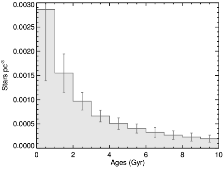
Figure 14.— The age distribution for our sample, constructed by applying our derived age-activity relation found in Section 6.2. The large error bars at young ages reflect the sensitivity of the age distribution to the input parameters when they are varied according to their uncertainties.

6.4. Implications for Habitability

Our analysis indicates an era of saturated NUV emission for young M dwarfs lasting $\sim$100–200 Myr (although possibly up to $\sim$$300$ Myr; see Shkolnik & Barman 2014). Roughly 120 stars in our sample have sufficiently high NUV luminosities ($R^{*}_{\rm NUV}\gtrsim 2.3\times 10^{-6}$ or $m_{\rm NUV}-K_{\rm S}\lesssim 10.9$) to place them in this saturation age interval. Correcting for a FP rate of $\sim$$25\%$ (see Figure 12) reduces this saturated sample to $\sim$90 stars or $\sim$$2\%$ of our sample. Any planets in the habitable zones of these young M dwarfs will be exposed to persistent, elevated NUV irradiation. Because the dissociation energies of several key atmospheric molecules are in the NUV (e.g., H₂O at 2398Å, CO₂ at 2247Å, CH₄ at 2722Å), the atmospheres of these planets can be significantly altered by photodissociation. Although detailed studies of these processes are just beginning, recent results suggest the implications may be significant (e.g., see Miguel et al. 2014 for the effects of Lyman $\alpha$ radiation on the atmosphere of mini-Neptune GJ 436b, which orbits an M3 star).

The saturation timescale of a few hundred Myr also roughly corresponds to the final “giant impact” phase predicted by terrestrial planet formation models. This interval scales with orbital period, which is proportionally shorter for planets in the compact habitable zones of M dwarfs (Morbidelli et al., 2012). This coincidence implies that the early atmospheres of planets around young M dwarfs are subject to erosion via heat injection from impactors in addition to NUV irradation by their host stars.

We also find that the vast majority of stars in our saturated sample ($\sim$70% after FP correction) have F_FUV/F${}_{\rm NUV}\geq 0.1$, which is at least two orders of magnitude above the solar value of $\sim$0.001 (see also France et al. 2013). This raises the potential for high rates of abiotic atmospheric O₂ and O₃ (produced from CO₂)—two molecules that have been proposed as biosignatures on Earth-like planets (see Tian et al., 2014, and references therein). Moreover, even some of the older M dwarfs in our sample, which exhibit basal levels of NUV emission above model-predicted photospheric values (see Figure 3), have F_FUV/F${}_{\rm NUV}\geq 0.1$. Thus very blue light may remain an important consideration for habitable-zone planets around these very red stars.

7. SUMMARY

We have constructed a NUV luminosity function for young, early-M dwarf stars. We cross-correlated the Lépine & Gaidos (2011) catalog of bright M dwarfs with the GALEX all-sky catalog of NUV sources to identify a sample of 4805 NUV-detected early-M dwarfs (M0-M3). Of these, 797 had NUV emission significantly ($>2.5\sigma$) in excess of an observed basal emission level; parameters of these candidate young stars are summarized in Table 4. When constructing the NUV luminosity function from this sample, we corrected for false positives (i.e., systems appearing NUV-luminous for reasons other than stellar youth; Section 4), the biases of the source catalogs toward intrinsically brighter sources (Section 5.2), and GALEX upper limits (Section 5.3). Key findings from our analysis are:

• Plotting $V-J$ (a proxy for stellar effective temperature) vs. $m_{\rm NUV}-K_{\rm S}$ (a measure of NUV luminosity) for our sample of 4805 NUV-detected early-M dwarfs shows two distinct populations. The majority of sources fall along a locus, but about 20% of the sample appears NUV luminous with $m_{\rm NUV}-K_{\rm S}$ colors at least 2.5$\sigma$ ($\sim$1.12 magnitudes) bluer than the main locus.

• All sources in our sample appear to exhibit a basal level of NUV emission above the expected photospheric value predicted by atmospheric models. This basal level of NUV emission for all M dwarfs regardless of age was first noted by Stelzer et al. (2013). Our empirical fit to this basal level of NUV emission as a function of $V-J$ color is $m_{\rm NUV}-K_{\rm S}=7.72+1.66(V-J)$.

• We conducted an extensive search for false positives (i.e., systems appearing NUV-luminous for reasons other than stellar youth) using medium-resolution optical spectra, high-resolution adaptive optics imaging, time-series photometry, and literature searches. We applied a maximum likelihood scheme to estimate the overall occurrence of false positives in our NUV-luminous sample to be $\sim$16%. However, we also found that this false-positive rate is significantly higher for the most NUV-luminous sources, reaching $\sim$80% by $m_{\rm NUV}-K_{\rm S}\sim 10$.

• We derived a NUV luminosity function for young, early-M dwarfs that was corrected for false positives, the biases of the source catalogs toward intrinsically brighter sources, and GALEX upper limits. Our derived NUV luminosity function is inconsistent with predictions from a constant star-formation rate and age-activity relation described by a two-parameter power law.

• We derived a NUV age-activity relation using the 20 YMG members in our sample with known ages as well as 28 older field stars identified by their high space motions. Results indicate a saturated NUV emission level for young, early-M dwarfs until $160\pm 70$ Myr of age, after which NUV emission declines with a power-law slope of $-0.83\pm 0.11$ (consistent with Shkolnik & Barman 2014 and Stelzer et al. 2013). However, because even the oldest stars in our sample exhibit basal levels of NUV emission above predicted photospheric values, this power-law decline in NUV emission is likely only applicable to a few Gyr of age.

8. ACKNOWLEDGEMENTS

MA and EG acknowledge support from NASA grants NNX10AQ36G (Astrobiology: Exobiology & Evolutionary Biology) and NNX11AC33G (Origins of Solar Sytem). This research utilized the NASA Astrophysics Data System, SIMBAD database, and Vizier catalogue access tool. It also made use of the AAVSO Photometric All-Sky Survey, funded by the Robert Martin Ayers Sciences Fund. We thank the dedicated staff of the UH88, MDM, SAAO, and CASLEO observatories from which many spectra were obtained for this work. We especially thank Greg Aldering for years of assistance with SNIFS on the UH88. We also thank Evgenya Shkolnik for her very useful comments regarding GALEX. This paper used observations taken with the Robo-AO system. The Robo-AO system is supported by collaborating partner institutions, the California Institute of Technology and the Inter-University Centre for Astronomy and Astrophysics, by the National Science Foundation under Grant Nos. AST-0906060, AST-0960343, and AST-1207891, by a grant from the Mt. Cuba Astronomical Foundation and by a gift from Samuel Oschin. C. B. acknowledges support from the Alfred P. Sloan Foundation.

Table 4Parameters of UV-luminous Early-M Dwarfs

Star	$V$	$J$	$m_{\rm NUV}-K_{\rm S}$	$F_{\rm NUV}$ ($\mu$Jy)	$F_{\rm FUV}$ ($\mu$Jy)	$F_{\rm X}$ (ergs cm-2 s-1)	EWHα (Å)	$\log(R^{\prime}_{\rm NUV})$	Robo-AOa	Low H$\alpha$b	Shifted H$\alpha$c	SuperWASPd	FP?e
PM_I00001+6943	13.52	9.70	10.95	44.04	99.99	2.95E-13	99.99	-5.67	—	—	—	—	N
PM_I00024-4601	12.43	9.18	11.98	27.05	5.78	99.99	99.99	-6.22	—	—	—	No	N
PM_I00059+4129	12.96	9.40	11.56	33.08	10.22	99.99	1.14	-7.48	No	No	No	Yes	D
PM_I00072-1036	11.85	8.83	11.29	70.18	11.78	4.48E-13	0.80	-5.89	—	No	No	—	N
PM_I00107-2039	13.39	9.48	11.18	43.77	10.82	9.27E-13	99.99	-5.77	—	—	—	—	N
PM_I00117-1139	12.67	9.85	11.05	34.89	99.99	99.99	-0.04	-5.83	—	No	—	—	N
PM_I00118-5521	13.34	9.32	11.50	36.21	18.78	99.99	3.18	-5.86	—	No	—	—	N
PM_I00162+1951W	11.79	7.88	11.64	117.08	22.29	2.39E-12	6.16	-5.90	—	No	—	—	N
PM_I00166+3000	12.79	9.11	12.42	20.21	3.56	1.02E-13	99.99	-6.38	—	—	—	—	N
PM_I00197-2233	13.77	9.88	12.44	9.59	99.99	99.99	99.99	-6.33	—	—	—	—	N
PM_I00206-5340	13.80	9.68	13.30	5.18	99.99	99.99	99.99	-6.71	—	—	—	—	N
PM_I00211+4456	13.62	9.60	10.89	52.93	99.99	1.07E-12	5.20	-5.67	No	No	No	—	N
PM_I00216-4605	12.21	8.32	11.14	133.11	28.10	7.46E-12	1.94	-5.76	—	No	—	No	N
PM_I00234+2418	13.03	9.75	11.01	40.74	99.99	99.99	-0.31	-7.48	Yes	No	—	No	D
PM_I00235+0947S	12.75	9.79	10.59	56.81	10.92	99.99	-0.77	-7.48	No	No	Yes	—	D
PM_I00235+2014	11.00	8.14	10.84	193.75	99.99	1.35E-12	0.30	-7.48	No	No	Yes	No	D
PM_I00241-6211	11.33	8.38	11.00	144.75	32.66	1.04E-12	0.94	-7.48	—	No	—	—	L
PM_I00245-2522	13.62	9.84	11.29	29.08	5.05	3.07E-13	2.68	-5.84	—	No	No	No	N
PM_I00250-3646	12.46	8.64	12.00	42.38	12.20	9.64E-13	1.12	-7.48	—	No	—	No	L

^aYes = found as FP by Robo-AO FP detection technique (Section 4.2.1); No = not found as FP by Robo-AO FP detection technique; – = not observed by Robo-AO.
^bSame as (a) but for missing H$\alpha$ FP detection technique (Section 4.2.2).
^cSame as (a) but for shifted H$\alpha$ FP detection technique (Section 4.2.3).
^dSame as (a) but for SuperWASP FP detection technique (Section 4.3.4).
^eL = found as FP in literature (Section 4.1); D = found as FP using detection techniques (Section 4.2); N = not found as FP in literature or by FP detection techniques; R = removed from NUVLF (Section 5.2); Y = YMG member used in age-activity relation derivation (Section 6.2).
Table 4 is published in its entirety in the electronic edition of The Astrophysical Journal. A portion is shown here for guidance regarding its form and content.

References

- Aldering et al. (2002) Aldering, G., et al. 2002, in Society of Photo-Optical Instrumentation Engineers (SPIE) Conference Series, Vol. 4836, Survey and Other Telescope Technologies and Discoveries, ed. J. A. Tyson & S. Wolff, 61–72
- Allard et al. (2013) Allard, F., Homeier, D., Freytag, B., Schaffenberger, , W., & Rajpurohit, A. S. 2013, Memorie della Societa Astronomica Italiana Supplementi, 24, 128
- Avni et al. (1980) Avni, Y., Soltan, A., Tananbaum, H., & Zamorani, G. 1980, ApJ, 238, 800
- Baranec et al. (2014) Baranec, C., et al. 2014, The Astrophysical Journal Letters, 790, L8
- Baranec et al. (2013) Baranec, C., et al. 2013, Journal of Visualized Experiements, 72, e50021
- Barnes et al. (2011) Barnes, J. R., Jeffers, S. V., & Jones, H. R. A. 2011, MNRAS, 412, 1599
- Bergemann et al. (2014) Bergemann, M., et al. 2014, A&A, 565, A89
- Bianchi et al. (2014) Bianchi, L., Conti, A., & Shiao, B. 2014, Advances in Space Research, 53, 900
- Bianchi et al. (2011) Bianchi, L., Efremova, B., Herald, J., Girardi, L., Zabot, A., Marigo, P., & Martin, C. 2011, MNRAS, 411, 2770
- Bonatto & Bica (2011) Bonatto, C., & Bica, E. 2011, MNRAS, 415, 2827
- Browne et al. (2009) Browne, S. E., Welsh, B. Y., & Wheatley, J. 2009, PASP, 121, 450
- Caffau et al. (2011) Caffau, E., Ludwig, H.-G., Steffen, M., Freytag, B., & Bonifacio, P. 2011, Sol. Phys., 268, 255
- Cox & Reynolds (1987) Cox, D. P., & Reynolds, R. J. 1987, ARA&A, 25, 303
- Cruz et al. (2007) Cruz, K. L., et al. 2007, AJ, 133, 439
- Duquennoy & Mayor (1991) Duquennoy, A., & Mayor, M. 1991, A&A, 248, 485
- Ehrenfreund et al. (2002) Ehrenfreund, P., et al. 2002, in ESA Special Publication, Vol. 518, Exo-Astrobiology, ed. H. Lacoste, 9–14
- Erkaev et al. (2013) Erkaev, N. V., et al. 2013, Astrobiology, 13, 1011
- Findeisen et al. (2011) Findeisen, K., Hillenbrand, L., & Soderblom, D. 2011, AJ, 142, 23
- France et al. (2013) France, K., et al. 2013, ApJ, 763, 149
- Gaidos et al. (2014a) Gaidos, E., et al. 2014a, MNRAS, 437, 3133
- Gaidos et al. (2007) Gaidos, E., Haghighipour, N., Agol, E., Latham, D., Raymond, S., & Rayner, J. 2007, Science, 318, 210
- Gaidos et al. (2014b) Gaidos, E., et al. 2014b, MNRAS, 443, 2561
- Gastine et al. (2013) Gastine, T., Morin, J., Duarte, L., Reiners, A., Christensen, U. R., & Wicht, J. 2013, A&A, 549, L5
- Gizis et al. (2002) Gizis, J. E., Reid, I. N., & Hawley, S. L. 2002, AJ, 123, 3356
- Hawley et al. (2002) Hawley, S. L., et al. 2002, AJ, 123, 3409
- Henden et al. (2012) Henden, A. A., Levine, S. E., Terrell, D., Smith, T. C., & Welch, D. 2012, Journal of the American Association of Variable Star Observers (JAAVSO), 40, 430
- Hernandez et al. (2000) Hernandez, X., Valls-Gabaud, D., & Gilmore, G. 2000, MNRAS, 316, 605
- Kouzuma & Yamaoka (2010) Kouzuma, S., & Yamaoka, H. 2010, MNRAS, 405, 2062
- Lantz et al. (2004) Lantz, B., et al. 2004, in Society of Photo-Optical Instrumentation Engineers (SPIE) Conference Series, Vol. 5249, Optical Design and Engineering, ed. L. Mazuray, P. J. Rogers, & R. Wartmann, 146–155
- Law et al. (2014) Law, N. M., et al. 2014, ApJ, 791, 35
- Leggett et al. (2001) Leggett, S. K., Allard, F., Geballe, T. R., Hauschildt, P. H., & Schweitzer, A. 2001, ApJ, 548, 908
- Lépine & Gaidos (2011) Lépine, S., & Gaidos, E. 2011, AJ, 142, 138
- Lépine et al. (2013) Lépine, S., Hilton, E. J., Mann, A. W., Wilde, M., Rojas-Ayala, B., Cruz, K. L., & Gaidos, E. 2013, AJ, 145, 102
- Lépine & Shara (2005) Lépine, S., & Shara, M. M. 2005, AJ, 129, 1483
- Malo et al. (2013) Malo, L., Doyon, R., Lafrenière, D., Artigau, É., Gagné, J., Baron, F., & Riedel, A. 2013, ApJ, 762, 88
- Mamajek (2012) Mamajek, E. E. 2012, ApJ, 754, L20
- Mann et al. (2012) Mann, A. W., Gaidos, E., Lépine, S., & Hilton, E. J. 2012, ApJ, 753, 90
- Markwardt (2009) Markwardt, C. B. 2009, in Astronomical Society of the Pacific Conference Series, Vol. 411, Astronomical Data Analysis Software and Systems XVIII, ed. D. A. Bohlender, D. Durand, & P. Dowler, 251
- Martin et al. (2005) Martin, D. C., et al. 2005, ApJ Letters, 619, L1
- Meibom et al. (2006) Meibom, S., Mathieu, R. D., & Stassun, K. G. 2006, ApJ, 653, 621
- Miguel et al. (2014) Miguel, Y., Kaltenegger, L., Linsky, J. L., & Rugheimer, S. 2014, ArXiv e-prints
- Morbidelli et al. (2012) Morbidelli, A., Lunine, J. I., O’Brien, D. P., Raymond, S. N., & Walsh, K. J. 2012, Annual Review of Earth and Planetary Sciences, 40, 251
- Norton et al. (2011) Norton, A. J., et al. 2011, A&A, 528, A90
- Perryman & ESA (1997) Perryman, M. A. C., & ESA, eds. 1997, ESA Special Publication, Vol. 1200, The HIPPARCOS and TYCHO catalogues. Astrometric and photometric star catalogues derived from the ESA HIPPARCOS Space Astrometry Mission
- Pollacco et al. (2006) Pollacco, D. L., et al. 2006, pasp, 118, 1407
- Rajpurohit et al. (2013) Rajpurohit, A. S., Reylé, C., Allard, F., Homeier, D., Schultheis, M., Bessell, M. S., & Robin, A. C. 2013, A&A, 556, A15
- Rebassa-Mansergas et al. (2013) Rebassa-Mansergas, A., Schreiber, M. R., & Gänsicke, B. T. 2013, MNRAS, 429, 3570
- Reiners (2012) Reiners, A. 2012, Living Reviews in Solar Physics, 9
- Reiners & Mohanty (2012) Reiners, A., & Mohanty, S. 2012, ApJ, 746, 43
- Ribas et al. (2005) Ribas, I., Guinan, E. F., Güdel, M., & Audard, M. 2005, ApJ, 622, 680
- Ricker (2014) Ricker, G. R. 2014, in Search for Life Beyond the Solar System. Exoplanets, Biosignatures, and Instruments, ed. D. Apai & P. Gabor, 3
- Rodriguez et al. (2011) Rodriguez, D. R., Bessell, M. S., Zuckerman, B., & Kastner, J. H. 2011, ApJ, 727, 62
- Rodriguez et al. (2013) Rodriguez, D. R., Zuckerman, B., Kastner, J. H., Bessell, M. S., Faherty, J. K., & Murphy, S. J. 2013, ApJ, 774, 101
- Rotchschild (1999) Rotchschild, L. J. 1999, Journal of Eukaryotic Microbiology, 46, 548
- Scalo et al. (2007) Scalo, J., et al. 2007, Astrobiology, 7, 85
- Scargle (1987) Scargle, J. 1987, in Bulletin of the American Astronomical Society, Vol. 19, Bulletin of the American Astronomical Society, 829
- Schmidt (1968) Schmidt, M. 1968, ApJ, 151, 393
- Schmitt et al. (1995) Schmitt, J. H. M. M., Fleming, T. A., & Giampapa, M. S. 1995, ApJ, 450, 392
- Shkolnik et al. (2009) Shkolnik, E., Liu, M. C., & Reid, I. N. 2009, ApJ, 699, 649
- Shkolnik & Barman (2014) Shkolnik, E. L., & Barman, T. S. 2014, AJ, 148, 64
- Shkolnik et al. (2011) Shkolnik, E. L., Liu, M. C., Reid, I. N., Dupuy, T., & Weinberger, A. J. 2011, ApJ, 727, 6
- Skrutskie et al. (2006) Skrutskie, M. F., et al. 2006, AJ, 131, 1163
- Stelzer et al. (2013) Stelzer, B., Marino, A., Micela, G., López-Santiago, J., & Liefke, C. 2013, MNRAS, 431, 2063
- Tarter et al. (2007) Tarter, J. C., et al. 2007, Astrobiology, 7, 30
- Tian (2009) Tian, F. 2009, ApJ, 703, 905
- Tian et al. (2014) Tian, F., France, K., Linsky, J. L., Mauas, P. J. D., & Vieytes, M. C. 2014, Earth and Planetary Science Letters, 385, 22
- Tremblay et al. (2014) Tremblay, P.-E., Kalirai, J. S., Soderblom, D. R., Cignoni, M., & Cummings, J. 2014, ApJ, 791, 92
- Voges et al. (1999) Voges, W., et al. 1999, A&A, 349, 389
- Voges et al. (2000) —. 2000, IAU Circ., 7432, 3
- West et al. (2008) West, A. A., Hawley, S. L., Bochanski, J. J., Covey, K. R., Reid, I. N., Dhital, S., Hilton, E. J., & Masuda, M. 2008, AJ, 135, 785
- Wheatley et al. (2013) Wheatley, P. J., et al. 2013, in European Physical Journal Web of Conferences, Vol. 47, European Physical Journal Web of Conferences, 13002
- York et al. (2000) York, D. G., et al. 2000, AJ, 120, 1579
- Yuan et al. (2013) Yuan, H. B., Liu, X. W., & Xiang, M. S. 2013, MNRAS, 430, 2188