Testing volume independence of SU(N) pure gauge theories at large N

Abstract

In this paper we present our results concerning the dependence of Wilson loop expectation values on the size of the lattice and the rank of the SU(N) gauge group. This allows to test the claims about volume independence in the large N limit, and the crucial dependence on boundary conditions. Our highly precise results provide strong support for the validity of the twisted reduction mechanism and the TEK model, provided the fluxes are chosen within the appropriate domain.

1 Introduction

Gauge theories lie at the basis of our understanding of Particle Physics. They are also beautiful mathematical models which are full of rich phenomena, both perturbative and non-perturbative. The pure gluon version of the theory has no free parameters and its dynamics underlies many of the fascinating properties of the interaction of quarks, such as Confinement and chiral symmetry breaking. Despite having no scale in its formulation, the theory is not conformal invariant because a scale $\Lambda$ is generated by the mechanism of dimensional transmutation CW. All physical properties of the theory can then be expressed, depending on its dimensions, in the appropriate units given by powers of $\Lambda$. Observable quantities which involve large energy scales (with respect to $\Lambda$) can be calculated by perturbative methods, thanks to the property of asymptotic freedom politzer-GW. On the contrary, if some low energy phenomena is involved, perturbation theory fails dramatically and one has to use non-perturbative techniques. Fortunately a very powerful formulation was introduced by K. Wilson wilson, allowing the development of several non-perturbative methods of computation. Lattice gauge theories define the quantum field theory as the limit of an statistical mechanical system at critically. One can then employ numerical methods which were originally devised to handle statistical mechanical systems. Unfortunately, for the study of the critical behaviour only numerical Monte Carlo methods seem useful. Nonetheless, progress in computer technology and in numerical algorithms have made possible the calculation of several observables of Yang-Mills and the more demanding theories with dynamical fermions (for recent results see Ref. latticeconf).

In the 70’s G. ‘t Hooft LN suggested the use of a new expansion parameter: $1/N$, the inverse of the rank of the group. Asymptotic freedom, Confinement, dimensional transmutation and a massive spectrum are still present at the lowest order approximation: the large N limit. Furthermore, it is known that several aspects of the theory are simpler in that limit: planar graphs, stable spectrum, factorisation migdal, etc. It seems clear that a more profound understanding of the large N limit would precede that of finite N. The large N limit also plays a crucial simplificatory role in the new ideas and methods that have emerged under the heading of AdS/CFT ads.

One of the obvious questions is then whether the large N limit also introduces a simplification in combination with the lattice gauge theory formulation. At first, it seems just the opposite. Numerical methods are devised to work with finite N values. Results at the large N limit then follow from extrapolating those obtained at finite $N$. But, the numerical effort grows with the number of degrees of freedom (hence, at least, as $N^{2}$). Nevertheless, following this procedure might be worth the effort, in order to produce predictions that can be matched with those of other approaches. A large literature has been generated following this line which can be consulted in Ref. LP.

There is, however, one potentially simplificatory phenomenon which was discovered when combining large $N$ with the lattice approach: reduction or volume independence. The idea emerged from a crucial observation made by Eguchi and Kawai(EK) EK when looking at the loop equations migdalmakeenko obeyed by Wilson loops on the lattice. Assuming invariance under $Z^{4}(N)$ centre symmetry and factorisation, they concluded that these equations are independent of the lattice volume.

Thus, if the phenomenon is correct, one can reduce the study of the large N limit to a simple matrix model with only $d$ matrices ($d$ is the space-time dimension). This is, no doubt, a very powerful simplification, at least at the conceptual level. The first question is then whether the idea is indeed correct. However, there are other secondary questions which could be crucial for applications. In particular, one might inquire about the size and nature of the corrections. What are the leading corrections that one has at large but finite N? These are the central issues which our paper tries to address.

The history of the subject is long. The initial stages took place soon after the EK paper. It was shown that the EK model, obtained by reducing to a one-point lattice with periodic boundary conditions, violates the centre-symmetry condition for reduction at weak coupling bhanot. Indeed, the one point lattice had been studied before the EK paper in Ref. gajka, and the weak coupling path integral was shown to be dominated by symmetry breaking configurations. Fortunately, the authors of Ref. bhanot proposed a modification under the name Quenched Eguchi-Kawai model (QEK) devised to restore the symmetry and, hence, the validity of reduction. On the other hand, the studies of Ref. gajka suggested that boundary conditions have a very strong influence on the weak coupling behaviour at finite volume. Thus, the present authorsTEK1-TEK2 presented a new version of reduction based upon twisted boundary conditions and aimed at respecting a sufficiently large subgroup of the centre symmetry group. The new model, called Twisted Eguchi-Kawai model (TEK), follows by imposing twisted boundary conditions and subsequently reducing the model to one point. At large volumes the boundary conditions do not influence the dynamics of the model, but at small volumes they are crucial.

Both the QEK and the TEK model passed all tests of absence of centre symmetry breaking done at the time of their proposal, and looked as valid implementations of the reduction idea. Unfortunately, attempts to solve these models explicitly failed. With an increasing interest in large N gauge theories the situation was re-examined in recent times, and signals of symmetry breaking were observed in both cases. By construction the QEK model is invariant under a certain subgroup of the $Z^{4}(N)$ group. However, there are possible subgroups associated with the action on several directions simultaneously that can be violated and were observed to do so in Ref. sharpe. In the case of the TEK model, although the remnant symmetry cannot be broken at infinite weak coupling, it can still be broken at intermediate values. The first observations of breaking were obtained by one of the present authors and collaborator TIMO. Later on, several other authors TV-Az confirmed the breaking and showed how this problem affects crucially the possibility of reduction in the continuum limit.

During these years there have been other attempts to recover the validity of the reduction idea and its simplificatory character. Some authors argued that other large N gauge theories might be free from the symmetry breaking problems that invalidated the reduction of the EK model. In particular, theories with several flavours of fermions in the adjoint representation KUY are good candidates. This has triggered several efforts to obtain information about these theoretically interesting theories, by benefiting from the computational advantage of their reduced versions AHUY; BS2; BKS; HN1; HN2; AGAMOAdj1; AGAMOAdj2; AGAMOAdj3. Although this is certainly very interesting, here we will not consider these theories any further since our interest in this paper is centred upon pure gauge theories.

Another approach was proposed by Narayanan and Neuberger NN, lately referred as partial reduction. The idea is to combine space and group degrees of freedom in an efficient way. Their study shows that at any value of the coupling there is a range of values of $L$ ($L$ being the linear size of the lattice box) for which the symmetry is respected at large $N$. More precisely, there is a minimum box size $L_{c}(b)$, which grows as the coupling gets weaker. Infinite volume large $N$ results can be approached by tuning $L$ and $N$ appropriately. Although this idea was mostly developed with periodic boundary conditions, it is also possible to combine it with twisted boundary conditions GANN. This is a possibility that we will analyse further in the present paper.

Reasons for the failure of the TEK model were given in Ref. TIMO-TV. Starting from these studies, the present authors proposed a simple modification of the original procedure which could restore the symmetry and recover the validity of reduction TEK3. The idea is to tune the fluxes appropriately when taking the large $N$ limit. Indeed, the twisted boundary conditions are not unique; they depend upon the choice of discrete fluxes through each plane. In Ref. TEK2 we determined the range of fluxes that guarantee the preservation of the symmetry at very weak coupling. However, it is now clear that the actual choice of fluxes within this range has an influence at intermediate values of the coupling. In Ref. TEK3 we argued that, with a suitable choice, the problems can be avoided at all values of the coupling.

In the last few years we have set up a program to study this problem. As explained earlier, the question is two-fold: Is reduction correct? Is it useful? The second aspect might be crucial for its ultimate interest as a valid simplification. Trying to answer the second question directly, we set ourselves the goal of computing an observable of the large $N$ continuum infinite volume theory using the TEK model. For simplicity we focused on the behaviour of large Wilson loops and the string tension. In parallel with the use of the reduced model, we also used the traditional extrapolation methodology to obtain the same quantity. Our comparison was presented in Ref. TEK4-TEK5, and showed that the extrapolation of the finite $N$ string tension agreed within the percent level with the quantity obtained from the reduced model. The result also matched reasonably well with other determinations of the large N string tension ATT-lohmayer.

Obtention of the continuum string tension is an elaborate procedure involving noise reduction techniques on the raw data, extrapolation to large size Wilson loops and then to the continuum limit. All of these steps, as well as the traditional methodology, involve extrapolations. This is always a dangerous arena, although it could hardly be a coincidence that the results match so well. Our initial focus on continuum results is understandable, since after all the lattice is primarily a method to obtain properties of the continuum formulated Yang-Mills theory. However, the reduction idea should be also valid for the lattice model itself, even away from criticality. In this paper we want precisely to look into that. We will focus upon simple observables of the lattice theory. Some are robust, highly precise, and devoid of any technical issues which might shade the validity of the result. Thus, rather than testing reduction by checking the preservation of the symmetry needed to validate the original proof, we will produce a direct test by comparing the volume independence of the corresponding observables. Furthermore, this is a quantitative comparison which can put limits on the errors committed. Ultimately, these errors are crucial for a precision determination of observables.

What do we know about the finite $N$ corrections to reduction? Perturbation theory gives some information in this respect. The propagators of the TEK model turn out to be identical to those of a lattice of size $(\sqrt{N})^{4}$ TEK2. This is reasonable since we are essentially mimicking the space-time degrees of freedom by those of the group. This seems more efficient than the equivalent counting for the QEK model, which suggests an effective volume of $(N^{1/4})^{4}$. Furthermore, if we opt for partial reduction in the twisted case, the effective length of the box is given by $L\sqrt{N}$. In addition to the effect on the propagators, the Feynman rules for the vertices also adopt a peculiar form. The structure constants turn into complex phases which depend on the “effective momentum” degrees of freedom. It is precisely this structure which suppresses the non-planar diagrams of the theory. The choice of flux enters the explicit form of the phase factors through a particular rational number in the exponent. Since all the factors cancel out for planar diagrams we were guided into thinking that the choice of fluxes was irrelevant. Now we know that this choice might be crucial in guaranteeing the preservation of centre symmetry. Recently GPGAO1; GPGAO2; GPGAO3; GPGAO4 we examined the problem with more detail for the simpler case of the 2+1 dimensional gauge theory. Physical observables seem to depend smoothly on the rational factor. This suggests a stronger form of volume independence valid at finite $N$. According to the previous considerations, as long as we preserve the effective spatial size ($LN$ in 2 dimensions) and the rational factor in the exponent of the vertices, we can trade spatial degrees of freedom by group degrees of freedom after a suitable tuning of the fluxes. It would be interesting to examine the situation for the 3+1 dimensional theory.

An important new ingredient appeared on the scene after the scientific community generated interest into quantum field theories in non-commutative space-times (for a review see Ref. nekrasov). It turns out that the afore-mentioned Feynman rules of reduced models are a discretized version of those appearing in those type of theories, where the rational number mentioned earlier is just proportional to the non-commutativity parameter. Indeed, the continuous version of the rules were actually anticipated by a generalisation of the reduced model obtained by one of us AGAKA, and which captures the non-commutativity in its formulation. All these new connections suggest that the results obtained at finite $N$ might have an interpretation and a usefulness in their own right.

In the previous paragraphs we have set up the situation that acts as background of the present paper. In the next section we will present all the methodological details leading to our results. This includes the description of the models and the parameters involved in them, the observables that we are going to study and the details about the simulations. The following section contains the analysis of our results for Wilson loops. The paper ends with a short concluding section.

2 Pure gauge theory on a finite lattice

2.1 The Models

As mentioned in the introduction we will focus upon pure gauge lattice theory at finite volume. The dynamical variables of our theory are the link variables $U_{\mu}(n)$ which are elements of the SU(N) group. The index $\mu$ ranges over the 4 directions of space-time $0,1,2,3$, while $n$ runs through all points of an $L^{4}$ hypercubic lattice $\mathcal{L}$. The partition function of the model is given by

$$Z=\prod_{n\in\mathcal{L}}\prod_{\mu=0}^{3}\left(\int dU_{\mu}(n)\right)e^{-S(U_{\mu})}$$ (1)

where the link variables are integrated with the Haar measure of the SU(N) group, and $S$ is action of the model. In this paper we will choose the simplest version of the action, proposed by Wilson,

$$S_{W}(U_{\mu})=-bN\sum_{n\in\mathcal{L}}\sum_{\mu\neq\nu}\mathrm{Tr}(U_{\mu\nu}(n))$$ (2)

where $U_{\mu\nu}(n)$ is the unitary matrix corresponding to an elementary plaquette starting at point $n$ and living in the $\mu-\nu$ plane. Its expression in terms of the link variables is

$$U_{\mu\nu}(n)=U_{\mu}(n)U_{\nu}(n+\hat{\mu})U^{\dagger}_{\mu}(n+\hat{\nu})U^{\dagger}_{\nu}(n)$$ (3)

where $\hat{\mu}$ is the unit vector in the $\mu$ direction. The lattice coupling $b$ is the lattice counterpart of the inverse of ‘t Hooft coupling $\lambda=g^{2}N$. Thus, the large $N$ limit has to be taken keeping $b$ fixed. In the previous formulas, we assumed periodic boundary conditions for the variables: $U_{\mu}(n+Lm)=U_{\mu}(n)$, for any integer vector $m$. Thus, the lattice is rather a toroidal one.

Wilson action is invariant under gauge transformations of the link variables:

$$U_{\mu}(n)\longrightarrow\Omega(n)U_{\mu}(n)\Omega^{\dagger}(n+\hat{\mu})$$ (4)

where $\Omega(n)$ are arbitrary SU(N) matrices. All physical observables are required to be gauge invariant. This property allows to relax the periodicity condition to

$$U_{\mu}(n+Lm)=\Omega(n,m)U_{\mu}(n)\Omega^{\dagger}(n+\hat{\mu},m)$$ (5)

To make this formula well-defined, the same gauge transformation has to result from two different ways to reach the same replica point. Since matrices do not necessarily commute, this implies consistency conditions to be satisfied by the gauge transformation matrices $\Omega(n,m)$. In particular, one can consider $n$ being the origin and $m=\hat{\mu}+\hat{\nu}$, and construct the gauge transformation in terms of the gauge transformations for $m=\hat{\mu}$ and $m=\hat{\nu}$. The consistency condition reads:

$$\Omega(L\hat{\mu},\hat{\nu})\Omega(0,\hat{\mu})=z_{\mu\nu}\Omega(L\hat{\nu},\hat{\mu})\Omega(0,\hat{\nu})$$ (6)

with $z_{\mu\nu}=\exp\{2\pi in_{\mu\nu}/N\}$ an element of the centre of the SU(N) group. Notice that if $n_{\mu\nu}=0$ for all planes, one can choose all $\Omega(n,\hat{\mu})$ to be the identity and we recover periodic boundary conditions. On the other hand, if some $n_{\mu\nu}\neq 0$ we get the so-called twisted boundary conditions introduced by ‘t Hooft TB. The integer $n_{\mu\nu}=-n_{\nu\mu}$ can be interpreted as a discrete flux modulo $N$ through the $\mu-\nu$ plane.

Now one can perform a change of variables to new link variables which are periodic at the expense of introducing a phase factor at certain plaquettes. The Wilson action now adopts the form

$$S_{W}(U_{\mu})=-bN\sum_{n\in\mathcal{L}}\sum_{\mu\neq\nu}z_{\mu\nu}(n)\mathrm{Tr}(U_{\mu\nu}(n))$$ (7)

The $z_{\mu\nu}(n)$ factors can be moved around depending on the change of variables, but their product over each plane cannot be changed. One possibility is to make all factors equal to one except for a single plaquette sitting at the corner of each plane. It is quite clear that for large volumes this has little influence in the local dynamics, but at small volumes it has an important effect.

An extreme situation occurs in reduced models. The lattice consists of a single point $L=1$. One can drop the $n$ dependence of links and plaquettes and one is left with a system involving only $d$ SU(N) matrices $U_{\mu}$. If one takes periodic boundary conditions one has the EK model. If, on the contrary, one chooses twisted boundary conditions, one has the TEK model. The latter has more freedom because one can take different values for the fluxes $n_{\mu\nu}$ having different properties. For a class of values there exist configurations having zero-action. Thus, in these cases, there exist matrices $U_{\mu}=\Gamma_{\mu}$ such that they satisfy

$$\Gamma_{\mu}\Gamma_{\nu}=z_{\nu\mu}\Gamma_{\nu}\Gamma_{\mu}$$ (8)

These are the twist-eaters gjka-AF. We will also impose the condition that the $\Gamma_{\mu}$ matrices generate an irreducible algebra. The interested reader can consult the literature to see the conditions imposed on the values of $n_{\mu\nu}$ to achieve this goal (see for example Ref. AGA). Rather than working with the most general case we will concentrate on a rather simple situation which tries to preserve as much symmetry as possible among the different directions: the symmetric twist. The situation occurs whenever $N$ is the square of an integer $N=\hat{L}^{2}$. Since, our goal is the large N limit, this restriction is not problematic. Furthermore, we will usually take $\hat{L}$ to be a prime number to avoid $Z(\hat{L})$ from having proper subgroups. In summary, for the symmetric twist case the twist factors for each plane are:

$$z_{\mu\nu}=e^{2\pi ik/\hat{L}}\quad\mathrm{for}\ \mu<\nu$$ (9)

where $\hat{L}=\sqrt{N}$ and $k$ is an integer defined modulo $\hat{L}$. Choosing $k=0$ we recover the case of periodic boundary conditions.

For completeness let us specify the form of the $\Gamma_{\mu}$ matrices for a symmetric twist with arbitrary $k\neq 0$. To do so, we first introduce two $\hat{L}\times\hat{L}$ matrices $P_{\hat{L}}$ and $Q_{\hat{L}}$ whose non-zero matrix elements are given by

$$P_{\hat{L}}(\ell,\ell+1)=1\ \ (\mathrm{for}\ 1\leq\ell\leq\hat{L}-1),\ \ P_{\hat{L}}(\hat{L},1)=1$$ (10)

$$Q_{\hat{L}}(\ell,\ell)=\exp{\pi ik\left[{1-\hat{L}\over\hat{L}}+{2(\ell-1)\over\hat{L}}\right]}\ \ (\mathrm{for}\ 1\leq\ell\leq\hat{L})$$ (11)

They are SU($\hat{L}$) matrices satisfying

$$P_{\hat{L}}Q_{\hat{L}}=\exp{\left({2\pi ik\over\hat{L}}\right)}Q_{\hat{L}}P_{\hat{L}}$$ (12)

The four $N\times N$ matrices $\Gamma_{\mu}$ with $N=\hat{L}^{2}$, are then given by the direct product of $P_{\hat{L}}$ and $Q_{\hat{L}}$ as follows

$$\Gamma_{0} = Q_{\hat{L}}\otimes Q_{\hat{L}}$$

$$\Gamma_{1} = Q_{\hat{L}}\otimes P_{\hat{L}}Q_{\hat{L}}$$

$$\Gamma_{2} = Q_{\hat{L}}\otimes P_{\hat{L}}$$ (13)

$$\Gamma_{3} = P_{\hat{L}}\otimes I_{\hat{L}}$$

with $I_{\hat{L}}$ the $\hat{L}\times\hat{L}$ unit matrix.

2.2 Observables

Now let us consider the main observables. The most natural gauge invariant observables are Wilson loops. A path on the lattice is a finite sequence of oriented links, such that the endpoint of one element in the sequence coincides with the origin of the next element. For each path we can construct a unitary matrix as a product of the associated link variables following, left to right, the order of the sequence. The reverse path is associated with the inverse matrix. A closed path is a path such that the endpoint of the last element in the sequence coincides with the origin of the first element. The trace of the corresponding unitary matrix is just the corresponding Wilson loop , which is gauge invariant.

It is clear that the simplest non-trivial closed path is an elementary plaquette $P_{\mu\nu}(n)$. The associated unitary matrix $U_{\mu\nu}(n)\equiv U(P_{\mu\nu}(n))$ has the expression given earlier (Eq. 3). The corresponding expectation value $E$ is the most precise lattice observable

$$E=\frac{1}{N}\langle\mathrm{Tr}(U_{\mu\nu}(n))\rangle$$ (14)

where the averaging is over positions, orientations and configurations. In pure gauge theories with Wilson action, the quantity is connected with the mean value of the action as follows

$$E=\frac{1}{Vd(d-1)bN^{2}}\langle S_{W}\rangle$$ (15)

where $V$ is the lattice volume and $d$ the space-time dimension.

For the case of twisted boundary conditions the change of variables into periodic link variables transforms the plaquette observable as follows:

$$U_{\mu\nu}(n)\longrightarrow z_{\mu\nu}(n)U_{\mu\nu}(n)$$ (16)

where the centre element $z_{\mu\nu}(n)$ is the same one appearing in the action. The above replacement in the formula for $E$ gives the correct expression with twisted boundary conditions.

A priori, $E$ is a function of the different parameters entering the simulation $E(b,N,L,n_{\mu\nu})$. Given its local character this quantity is expected to have a well-defined infinite volume limit which is independent of the boundary conditions: $E(b,N)$. On general grounds one expects it to have also a well-defined large $N$ limit $E_{\infty}(b)$, with corrections that go as powers of $1/N^{2}$.

Apart from the plaquette, one can consider other Wilson loops. Here we will focus on those associated to a rectangular path of size $R\times T$. The corresponding expectation value will be named $W(R,T)$. Once more, the quantity has to be modified in the standard variables for twisted boundary conditions. The modification is just to multiply the expression by the product of all $z_{\mu\nu}(n)$ factors for the plaquettes contained in the rectangle.

Just as for the plaquette, the expectation value will depend on $b$, $N$, $L$ and $n_{\mu\nu}$, but also depends on $R$ and $T$. One expects a well-defined thermodynamic limit as $L$ goes to $\infty$ at fixed $R$ and $T$. For obvious reasons, the finite volume corrections should be larger as $R$ and $T$ get closer to $L$. These corrections should depend on the boundary conditions. An extreme situation occurs for the reduced model. In that case, the loop extends beyond the size of the box:

$$W(R,T)=\frac{1}{N}z_{\mu\nu}^{RT}\langle\mathrm{Tr}(U_{\mu}^{R}U_{\nu}^{T}U_{\mu}^{-R}U_{\nu}^{-T})\rangle$$ (17)

Nevertheless, the statement of volume independence at large $N$ implies that even loops that extend beyond the size of the box should behave as those obtained at infinite volume.

2.3 Methodology

The numerical results presented in this paper were obtained using a heat-bath Monte Carlo simulation. For the Wilson action case, each link variable $U_{\mu}(n)$ has a distribution determined by the part of the action containing it, which has the form

$${\rm ReTr}\{U_{\mu}(n)V_{\mu}(n)\}$$ (18)

where $V_{\mu}(n)$ is constructed in terms of the neighbouring links. Thus, at each local update one should generate a new link according to the previous distribution. However, the constraint that $U_{\mu}(n)$ belongs to SU(N) complicates this task. As has been demonstrated in MO, a SU(N) link variable can be updated by successive multiplication of SU(2) sub-matrices. However, the standard Creutz’ s heat bath-algorithm has a very low acceptance rate for SU(N) gauge theories with N larger than 8. To avoid this, we have used a heat-bath algorithm proposed by Fabricius and Haan FH that significantly improves the acceptance rate for larger values of N.

Apart from this, there are two technical points which significantly speed up the SU(2) heat bath manipulations.

1. Suppose $A$ is an SU(2) sub-matrix, and we want to change the link variable as follows $U_{\mu}(n)^{\prime}=AU_{\mu}(n)$. During the updating step, we should also store $W=U_{\mu}(n)V_{\mu}(n)$, namely $W^{\prime}=AW$, which only requires $O(N)$ arithmetic.

2. An SU(N) matrix has $N(N-1)/2$ SU(2) sub-matrices (i,j). For odd(even) N, there are $n_{1}=N$ ($N-1$) sets having $n_{2}=(N-1)/2$ ($N/2$) (i,j) pairs, which can be manipulated simultaneously. For example, for N=5, we have the following 5 sets of two pairs: $\{(1,2),(3,4)\}$, $\{(1,3),(2,5)\}$, $\{(1,4),(3,5)\}$, $\{(1,5),(2,4)\}$, $\{(2,3),(4,5)\}$. If the computer supports vector or multi-core coding, we should make full use of these $n_{2}$ independent manipulations.

For the case of the reduced model (having $L=1$), the previous methodology fails, because the distribution is not given by Eq. 18. The part of the action containing $U_{\mu}(n)$ depends quadratically rather than linearly on it. However, one can return to a linear dependence by introducing a Gaussian random matrix, which after integrating over it reproduces the original form FH. Thus, we can alternate the updating of the new random matrix with the previous heat-bath update.

Finally a link update is obtained by applying the SU(2) update for each of the $N(N-1)/2$ SU(2) subgroups in SU(N). A sweep is obtained by applying an update for all the links on the lattice, followed by 5 over-relaxation updates.

To reduce autocorrelations we typically measured configurations separated by 100 sweeps. In any case, the final errors were estimated by a jack-knife method with much larger separation among groups. Another important point concerns thermalization. Typically we discarded the initial 10% of our configurations. We monitored several quantities to ensure that we observed no transient effects in the resulting data. Related to this point there is the choice of initial configuration. For the TEK model we always initiated thermalization from the cold configuration that minimises the action at weak coupling $U_{\mu}=\Gamma_{\mu}$. We observed no sign of phase transition behaviour except for low values of $b$ and small $N$. Indeed, some of our results extend below the transition point between strong and weak coupling, which was estimated to be $b=0.3596(2)$ in Ref. campostrini. Results below this value of $b$ lie then in a metastable phase (at infinite $N$). Nonetheless, it seems that as $N$ grows the probability of tunnelling decreases considerably and there are no signs of phase flips even down to $b=0.35$. Whether the tests of volume independence are performed in a metastable region or not is of no particular concern, as was the case for the partial reduction studies of Ref. NN. The same applies for the other phases presented in the same reference. In all our simulations we have monitored the behaviour of open loops which are not invariant under the $Z(\sqrt{N})^{4}$ symmetry of the reduced model and found them to be compatible with zero within errors. As mentioned in the introduction, the choice of flux $k$ is obviously crucial for this result. Our results, therefore, provide a test that the criteria, presented in Ref. TEK3 to avoid symmetry breaking, works well.

Finally, a comment about the total statistics and computer resources employed in our results. The number of different simulation parameters involved in our work are in the hundreds, and have been accumulated over several years. Typically, the number of configurations used for our large volume (L=16,32) periodic boundary conditions results is the range 300-600, and have been generated with INSAM clusters at Hiroshima University. For the TEK model we have used typically 6000 configurations at each $b$ value at N=841, and 2000 configurations at N=1369. The most extensive and computer-wise demanding results were obtained with the Hitachi SR16000 supercomputers at KEK and YITP. Some small scale results were obtained with the clusters and servers at IFT.

3 Size and N dependence of small Wilson loops

3.1 General considerations about volume independence

Expectation values of the lattice observables depend on the conditions of the simulations, namely the values of $b$, $L$, $N$ and the twist tensor $n_{\mu\nu}$. Restricting ourselves to the symmetric twists we may write $O(b,N,L,k)$ for a generic observable $O$. In the thermodynamic or infinite volume limit, local observables should have a well defined value:

$$\lim_{L\longrightarrow\infty}O(b,N,L,k)=O(b,N)$$ (19)

Notice that in that limit the dependence on the boundary conditions drops out. In general, we expect the infinite volume observable to have a well defined large $N$ limit:

$$\lim_{N\longrightarrow\infty}O(b,N)=O_{\infty}(b)$$ (20)

The observable $O_{\infty}(b)$ is the large N quantity that we are interested in.

The question now poses itself about the commutativity of the order of both limits. What is the result if we take large N limit first, and then the infinite volume limit? The concept of volume independence EK gives a striking answer to this question. Taken at face value it predicts

$$\lim_{N\longrightarrow\infty}O(b,N,L,k)=O_{\infty}(b)$$ (21)

Even before it was formulated this hypothesis, as such, was known to be wrong. Its validity depends upon the value of $b$ and the dimensionality of space-time. While presumably correct in two dimensions it is certainly not true in higher dimensions and sufficiently large values of $b$. Still the hypothesis is correct for $b$ in the strong coupling region $b<b_{c}(N)$ EKAGAST. The point brought into the discussion by Ref. TEK3 is about the dependence of the statement upon the value of $k$. No doubt that the choice of $k$ has a crucial influence on the results for small $L$. The proposal of Ref. TEK2 of choosing $k$ coprime with $\sqrt{N}$ avoids the problems found for $k=0$ (periodic boundary conditions) at small enough couplings (large $b$).

A modified hypothesis for the periodic boundary condition ($k=0$) case, known as partial reduction, was introduced by Narayanan and Neuberger NN. In view of their results, they conjectured that volume independence remains true provided $L>L_{c}(b)$, with $L_{c}(b)$ a growing and asymptotically divergent function of $b$. This idea can be combined with the use of twisted boundary conditions. Not surprisingly, the effective value of $L_{c}(b)$, as obtained in finite $N$ studies, seems to depend also on $k$ GANN.

However, numerical studiesTIMO-TV disproved the initial hypothesis that it is enough to take $k$ coprime with $\sqrt{N}=\hat{L}$ to restore volume independence, as formulated in Eq. 21, at all values of the coupling. In view of this, a modified volume independence proposal was put forward in Ref. TEK3:

$$\lim_{\hat{L}\longrightarrow\infty}O(b,N=\hat{L}^{2},L,k_{\hat{L}})=O_{\infty}(b)$$ (22)

This implies that the flux has to be scaled as $\hat{L}$ is sent to infinity. According to the proposal, based on centre symmetry breaking arguments, the precise value of $k_{\hat{L}}$ is not relevant provided $k_{\hat{L}}/\hat{L}$ and $\bar{k}_{\hat{L}}/\hat{L}$ remain always larger than a certain threshold ($\sim 0.1$). Here $\bar{k}$ is an integer such that $k\bar{k}=1\bmod\hat{L}$. The restrictions of working with symmetric twists and values of $N$ that are the square of an integer are presumably not indispensable. They emerge from the simplicity of maintaining as much isotropy as possible among the different directions of space-time.

The validity of any volume independence hypothesis has always been tested indirectly by verifying the $Z^{4}(N)$ symmetry condition assumed in Eguchi and Kawai proof. Although this is valid road-map, nowadays it is possible to explore directly how a given particular observable behaves as a function of the different quantities involved. This has the advantage of informing us of the rate at which the asymptotic limits are attained, which is a crucial piece of information in rendering volume independence a useful tool in numerical studies. In what follows we will present the results of our analysis taking as observables the best measured lattice observables: the plaquette and other small Wilson loops. One of the good things of the reduction or volume-independence hypothesis is that it is valid for the lattice theory, not only the continuum limit. If reduction takes place in the scaling region, this will be inherited by the continuum limit.

3.2 Behaviour at very weak coupling

Although most of our interest has concentrated in the region of $b$ values from which scaling results are obtained, it is interesting to examine what happens to volume independence at very weak couplings (large values of $b$). In that region, perturbation theory is a good approximation to the behaviour of our lattice quantities. Typically one gets an expansion of the form

$$O(b,N,L,k)=\hat{O}_{0}(N,L,k)-\sum_{n=1}^{\infty}\hat{O}_{n}(N,L,k)\frac{1}{b^{n}}$$ (23)

For Wilson loops the leading term is $\hat{O}_{0}(N,L,k)=1$.

Let us start by focusing upon the plaquette $E(b,N,L,k)$. The infinite volume coefficients up to order $n=3$ have been computed by several authors dGR-Alles. The corresponding values in 4 dimensions are

$$\hat{E}_{1}(N) = \frac{1}{8}(1-\frac{1}{N^{2}})$$ (24)

$$\hat{E}_{2}(N) = \frac{1}{24}(1-\frac{1}{N^{2}})(0.12256631-\frac{3}{16N^{2}})$$ (25)

$$\hat{E}_{3}(N) = (1-\frac{1}{N^{2}})(0.000794223-0.002265487/N^{2}+0.0023152583/N^{4})$$ (26)

The finite volume corrections for periodic boundary conditions started to be studied long time ago. The main difficulty is the presence of infinitely many gauge inequivalent configurations with zero-action: the torons gajka. If one expands around the trivial classical vacuum $A_{\mu}=0$ (which dominates the path integral for d=4 and large $N$), one must separate the fluctuations into those with zero momentum and the rest. The non-zero momentum contributions to the plaquette were studied in Ref. CPT-HellerKarsch. They adopt the form:

$$\hat{E}^{(p\neq 0)}_{1}(N,L,k=0)=\frac{1}{8}(1-\frac{1}{N^{2}})(1-\frac{1}{L^{4}})$$ (27)

The corresponding contribution of the zero-momentum degrees of freedom was computed in Ref. Coste. In 4 dimensions it becomes:

$$\hat{E}^{(p=0)}_{1}(N,L,k=0)=\frac{1}{12}(1-\frac{1}{N^{2}})\frac{1}{L^{4}}$$ (28)

It is clear that the leading order finite volume corrections do not cancel each other and do not go to zero as $N$ goes to infinity:

$$\hat{E}_{1}(N,L,k=0)=\frac{1}{8}(1-\frac{1}{N^{2}})(1-\frac{1}{3L^{4}})$$ (29)

This kills the volume independence hypothesis for periodic boundary conditions at weak coupling, where the calculation is reliable.

For twisted boundary conditions the calculation is very different since the action has isolated minimum action solutions. In this case the result is given by gajkaCoste

$$\hat{E}_{1}(N,L,k\neq 0)=\frac{1}{8}(1-\frac{1}{N^{2}})$$ (30)

Hence, there is no volume dependence at this order. This result, as well as that of periodic boundary conditions, can be easily derived since the expectation value of the plaquette can be obtained by differentiating the partition function with respect to $b$. To this order what matters is just the counting of gaussian and quartic fluctuations.

In the same references the volume dependence of rectangular $R\times T$ Wilson loops to leading order in perturbation theory was also studied. The infinite volume coefficients up to order $\lambda^{2}$ were computed in Ref. WWW. For loop sizes much smaller than the lattice size, the leading finite volume correction from non-zero momentum is

$$\delta\hat{W}^{(p\neq 0)}_{1}(R,T,N,L,k=0)=\frac{1}{8}(1-\frac{1}{N^{2}})\frac{R^{2}T^{2}}{L^{4}}+\mathcal{O}(L^{-6})$$ (31)

while the zero momentum one is

$$\delta\hat{W}^{(p=0)}_{1}(R,T,N,L,k=0)=\frac{1}{12}(1-\frac{1}{N^{2}})\frac{R^{2}T^{2}}{L^{4}}$$ (32)

Again they do not cancel each other, leaving a finite volume correction at all $N$. On the contrary the result for twisted boundary conditions takes the form

$$\hat{W}_{1}(R,T,N,L,k\neq 0)=\hat{W}^{(p\neq 0)}_{1}(R,T,N=\infty,L\hat{L},k=0)-\frac{1}{N^{2}}\hat{W}^{(p\neq 0)}_{1}(R,T,N=\infty,L,k=0)$$ (33)

where $\hat{L}=\sqrt{N}$. The first term is just the result of periodic boundary conditions at $N=\infty$ and a lattice volume of $N^{2}L^{4}$. Thus as $N$ grows we approach the infinite volume result irrespective of the value of $L$. The second term goes like $1/N^{2}$ in the large $N$ limit, but plays an important role in reducing finite volume corrections. This comes because the leading $L^{-4}$ corrections cancel each other between the first and second terms, so that the leading finite volume dependence in the sum goes like $N^{-2}L^{-6}$. Notice that, due to the same reason, adding the $p=0$ contribution to the $k=0$ coefficients of the right-hand side does not alter the result. In summary, large N volume independence holds at this order.

In Ref. TEK2 the present authors studied the structure of the Feynman rules for the TEK model ($L=1$) and argued that volume independence should hold at all orders of perturbation theory. This result trivially extends to large $N$, $k\neq 0$ models for any $L$. The rules are essentially a lattice version of those of non-commutative field theory. The finite $N$ corrections appear in two ways. On one side the propagators are just the lattice propagators in a box of size $L\sqrt{N}$. This relates finite $N$ effects with finite volume effects. However, in addition the finite $N$ effect comes in as a non-planar diagram contribution, which is generically exponentially suppressed with $N$, but might induce also power-like suppressions. Furthermore, the coefficients depend on the choice of the flux $k$. To quantify finite $N$ and finite volume corrections, including the effect of $k$, a numerical analysis of the $\mathcal{O}(\lambda^{2})$ coefficients would be quite interesting. This study is currently under way MGPAGAMO.

In the absence of explicit perturbative calculations, we might use numerical simulations at small coupling in order to quantify the size of finite volume corrections at weak coupling (large values of $b$). In this work we used limited resources, by taking $L=1,2,4$ and $N=49$ for both periodic and twisted boundary conditions. A more precise study will be performed to test the higher order analytic calculations.

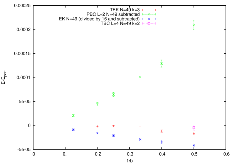
Figure 1: We plot the measured value of the plaquette $E$ minus the infinite volume perturbative result up to order $\lambda^{3}$ for $N=49$. The result for the TEK model (red points) is compatible with zero to within two sigma. For the periodic boundary conditions (L=1 blue and L=2 green) we subtracted the finite size corrections to order $\lambda$ and plotted the difference (divided by 16 for $L=1$).

Hence, we will compare our numerical results with the predictions of perturbation theory at infinite volume. The results for the plaquette expectation value at $b\geq 2$ and $k\neq 0$ are quite compatible with the perturbative formulas. For example, the perturbative prediction at infinite volume at $b=2$ and $N=49$ is $0.936152$, while the measured value for $L=4$ and a symmetric twist with $k=2$ is $0.936147(5)$. The difference is compatible with zero within errors, which are smaller than the $1/N^{2}$ corrections, since the perturbative value at $N=\infty$ gives $0.936123$. For the TEK model ($L=1$) one gets $0.936134(4)$, $0.936140(4)$, $0.936135(4)$ for $k=1,2,3$ respectively, which is in agreement with the $L=4$ result and within acceptable $1/b^{4}$ corrections of the perturbative value. We emphasise that the agreement is sensitive to the $\mathcal{O}(\lambda^{2})$ and higher perturbative coefficients. To see this, we fitted a cubic polynomial in $1/b$ to the plaquette results fixing the constant and linear coefficients to the perturbative infinite volume values. The best fit (having chi square per degree of freedom less than 1) gives a value $0.00511(3)$ for the coefficient in $1/b^{2}$, while the infinite volume coefficient is $0.005102$. The $1/b^{3}$ coefficient fits to a value of $0.00091(8)$ which is not far from the infinite volume result $0.000793$. The panorama is summarised in Fig. 1. In it we show the difference between the measured and three-loop (order $1/b^{3}$) infinite volume perturbative value of the plaquette for the TEK model ($L=1$) $N=49$ and $k=3$. Thus, within the precision of the numerical data we conclude that the plaquette of the Twisted Eguchi-Kawai model in the perturbative region is compatible with infinite volume perturbation theory already for $N=49$.

The previous result is in strong contrast with the result for periodic boundary conditions. We already found that there are sizeable finite volume corrections of order $\lambda=1/b$. However, even if we subtract out this contribution finite size effects are still considerably larger than for TEK. In Fig. 1 we show the case of $L=2$ $k=0$, and also the $L=1$ $k=0$, which has been divided by 16 to fit it into the same plot.

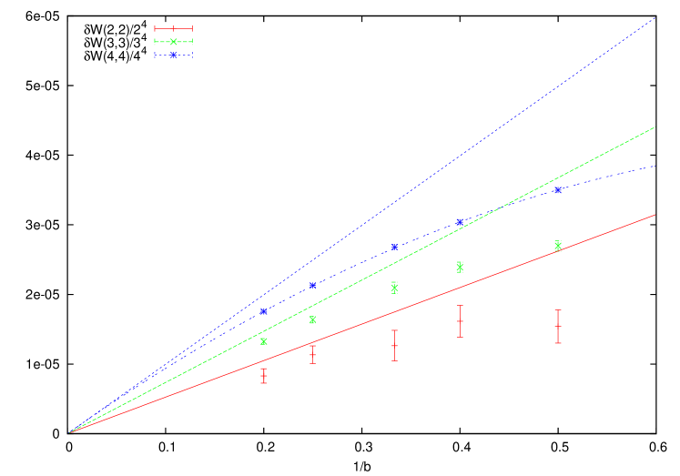
Figure 2: For the TEK model at $N=49$ and $k=3$ we plot $\delta W(R,R)$, the difference between the measured expectation values of Wilson loops and the next-to-leading perturbative formula at infinite volume. The result is divided by $R^{4}$ and compared with the analytic prediction at leading order (straight line in the same colour) and a second-degree polynomial fit for $R=4$.

It is also very interesting to look at what happens for larger loops. In contrast with the case of the plaquette, the result at lowest order has a non-vanishing finite size correction which, as we saw earlier, is of order $1/N^{2}$. The question is whether there is numerical evidence that higher orders violate this rule and produce large corrections. Again we have looked at the TEK model at $N=49$ and various $b\geq 2$ values. We measured the mean values of the Wilson loops and subtracted from it the perturbative formula for the infinite volume Wilson loop, up and including order $\lambda^{2}$. Hence, the difference $\delta W(R,T)$ measures the leading corrections to volume independence. Asymptotically this must be dominated by the term linear in $1/b$ which can be computed analytically, and which for very large $N$ and $R,T\ll\sqrt{N}$ is given by

$$-\frac{\lambda}{N^{2}}(\hat{W}_{1}(R,T,N=\infty)-\frac{R^{2}T^{2}}{8})+\mathcal{O}(\frac{1}{N^{3}})$$ (34)

Thus, the correction for $R=T$ grows with the fourth power of $(R/\sqrt{N})$. As expected $\sqrt{N}$ acts as the effective size of the box. Thus, in Fig.2 we plot our result for $\delta W(R,R)/R^{4}$ at $N=49$ with twisted boundary conditions and $k=3$. The straight lines are the leading order perturbative contribution. Since, $R=T=3,4$ are not much smaller than $\hat{L}=7$ the slopes for the various $R$ change by a factor of 2. The actual data lie always below the corresponding straight line, implying that higher powers of $1/b$ produce a dependence of the opposite sign. Indeed, one can easily describe the data points by simply adding a $1/b^{2}$ correction with a coefficient determined by a fit. The corresponding line is also plotted as the blue curve for $R=T=4$.

3.3 N-dependence of Plaquette at $b=0.36$

In what follows we move to the other edge of the weak coupling phase of the large N model. We choose a particular value of the coupling $b=0.36$, right above the strong to weak phase transition point. At this point we carried a large number of simulations to determine the expectation value of the plaquette for various values of $N$, $L$ and the flux $k$. As mentioned earlier, we expect that when $L$ is large enough, the result should be independent of the boundary conditions and given by $E(0.36,N)$. We estimate that at $L=16$ one gets a good measure of this quantity within the errors of order $0.00001$. In particular, for $N=8$, $L=16$ and $k=0$ (periodic boundary conditions) one gets $E(0.36,8,16,k=0)=0.572022(19)$, which is compatible with the value obtained at $N=8$, $L=32$ and $k=0$ given by $E(0.36,8,32,k=0)=0.572019(5)\sim E(0.36,8)$.

To test the volume independence hypothesis, we performed a series of simulations in a lattice of size $L^{4}=16^{4}$ with periodic boundary conditions, for $b=0.36$ and all values of $N$ in the range $N\in[8,16]$. The mean plaquette value results are displayed in Fig. LABEL:plaquette036a as a function of $1/N^{2}$. The dependence on $N$ is clearly visible, being much larger than the individual errors, which are too small to be seen in the plot. A good fit is obtained by a second degree polynomial in $1/N^{2}$. The $\chi^{2}$ per degree of freedom is 0.248, for 9 points and 3 parameters. The coefficient of the linear term is $0.960(3)$. The constant coefficient in the fit provides the extrapolated value of the plaquette at $N=\infty$, and its value is $E_{\infty}(0.36)=0.558012(12)$. To test the $L$ dependence we repeated the analysis in an $8^{4}$ and $4^{4}$ periodic box. The results of the $8^{4}$ box are numerically close to those of $16^{4}$, but the difference is much larger than the errors and clearly seen in the plot. For $N=8$ the difference is $3.41(70)\,10^{-4}$ and for $N=16$ it is $2.42(50)\,10^{-4}$. A similar three parameter fit describes the data very well and gives an extrapolation of $0.558114(67)$. Indeed, even fixing the extrapolated value to be equal to the $L=16$ one, we get a fit with a chi square per degree of freedom which is smaller than 1. Thus, our results are consistent with the basic claim that the volume dependence drops to zero in the large $N$ limit.

In contrast we also show the results of the $L=4$ periodic lattice. For this smaller volume we have explored values of $N=8,10,12,14,16,25,49,81$. A good polynomial fit can be obtained which undoubtedly extrapolates to a very different value in the large $N$ limit. Thus, volume independence fails in this case. This is precisely what we expected on the basis of the results of Narayanan and Neuberger NN. At $b=0.36$ volume independence should only work for $L\geq L_{c}(0.36)\sim 8$.