Chaos in high-dimensional dynamical systems

Abstract

For general dissipative dynamical systems we study what fraction of solutions exhibit chaotic behavior depending on the dimensionality $d$ of the phase space. We find that a system of $d$ globally coupled ODE’s with quadratic and cubic non-linearities with random coefficients and initial conditions, the probability of a trajectory to be chaotic increases universally from $\sim 10^{-5}-10^{-4}$ for $d=3$ to essentially one for $d\sim 50$. In the limit of large $d$, the invariant measure of the dynamical systems exhibits universal scaling that depends on the degree of non-linearity but does not depend on the choice of coefficients, and the largest Lyapunov exponent converges to a universal scaling limit. Using statistical arguments, we provide analytical explanations for the observed scaling and for the probability of chaos.

In many standard texts, a transition from classical concepts to statistical mechanics is justified by the prevalence of chaotic and ergodic behavior as more degrees of freedom are considered. However, quantitative details of such transitions from integrability to chaos apparently remain elusive. In this paper we consider the fundamental question of the likelihood of chaos in general dissipative dynamical systems in continuous time as a function of the dimension of phase space. We note that existing results about the probability of chaos vs. dimensions in discrete maps kaneko1984; kaneko1989; sprott2006 as well as in a Hamiltonian system of locally-coupled oscillators mulansky2011 cannot be applied to dissipative dynamical systems in continuous time with an arbitrary degree of non-linearity and global coupling. In the following we show that the probability that the solution of a generic $d$-dimensional system of ODEs with quadratic and cubic non-linearities (1,2,3) is chaotic universally increases from $\sim 10^{-4}-10^{-5}$ for $d=3$ to essentially $1$ for large $d$. The results of our numerical investigations are then explained analytically, using a combination of scaling and statistical methods. These results are an extension and generalization of an investigation of the prevalence of chaos in the dynamics of high-dimensional phenotypes under frequency-dependent natural selection id14. However, the applicability and significance of our results is not limited to biological evolution, and in principle extends to dynamical systems in statistical and nonlinear physics, hydrodynamics, plasma physics, control theory, and social and economic studies.

To investigate the statistics of trajectories, we numerically solve the following systems of equations which contain second- and third-order nonlinear terms of a general form,

$$\frac{dx_{i}}{dt}=\sum_{j=1}^{d}b_{ij}x_{j}+\sum_{j,k=1}^{d}a_{ijk}x_{j}x_{k}-x_{i}^{3},\;i=1,\ldots,d,$$ (1)

$$\frac{dx_{i}}{dt}=\sum_{j=1}^{d}b_{ij}x_{j}+\sum_{j,k=1}^{d}a_{ijk}x_{j}x_{k}+$$ (2)

$$+\sum_{j,k,l=1}^{d}c_{ijkl}x_{j}x_{k}x_{l}-x_{i}^{5},\;i=1,\ldots,d,$$

$$\frac{dx_{i}}{dt}=\sum_{j=1}^{d}b_{ij}x_{j}+\sum_{j,k=1}^{d}a_{ijk}x_{j}x_{k}+$$ (3)

$$+\sum_{j,k,l=1}^{d}c_{ijkl}x_{j}x_{k}x_{l}-x_{i}^{3}|x_{i}|,\;i=1,\ldots,d.$$

The coefficients $\{a\},\{b\},$ and $\{c\}$ were randomly and independently drawn from Gaussian distributions with zero mean and unit variance. The last highest-order terms, $-x_{i}^{3},\;-x_{i}^{5}$, and $-x_{i}^{3}|x_{i}|$ were introduced to ensure confinement of all trajectories to a finite volume of phase space, thus excluding divergent scenarios. In id14, we integrated system (1) for each dimension $d$ using a 4th-order Runge-Kutta method for 50 sets of the coefficients $b_{ij}$ and $a_{ijk}$, each with 4 sets of random initial conditions. This procedure was repeated for the current work. For (2) and (3), the numerical simulations are significantly more complex and computationally extensive. We therefore integrated systems (2) and (3) using a 5th-order Runge-Kutta adaptive step method for 50 - 100 sets of the coefficients $b_{ij}$, $a_{ijk}$ and $c_{ijkl}$ each with only a single set of random initial conditions. For each trajectory we determined the Largest Lyapunov Exponent (LLE) by perturbing the trajectory by a small magnitude $\delta x_{0}$ in a random direction, integrating both trajectories in parallel for time $\tau$, measuring the distance between trajectories $\delta x_{\tau}$, rescaling the separation between trajectories back to $\delta x_{0}$, and continuing this for the course of the simulation. The LLE was calculated as

$$\lambda=\frac{1}{\tau}\ln\left(\frac{\|\delta x_{\tau}\|}{\|\delta x_{0}\|}\right),$$ (4)

and subsequently averaged over the trajectory. The time of integration was chosen such that the average LLE saturated to a constant value and it was usually not less than $\sim 10^{4}/d^{\beta}$ with $\beta=2,\;3,\;9/2$ for Eqs.(1,2,3). We explain this scaling below. In cases when a trajectory converged to a stable fixed point and the LLE was persistently negative, the integration was stopped. By visually inspecting remaining trajectories we derived a fairly robust criterium, observing that trajectories with $\lambda\sim d^{\beta}$ (with the proportionality coefficient being of order of 0.1) are chaotic, while the trajectories with $\lambda\sim 1$ are “quasiperiodic”, i.e. converging to a limit cycle. Rather infrequent intermediate cases where inspected and classified individually. For Eq. (1) where simulations were less computationally-expensive, we were able to implement more refined method of estimating $l$, first allowing considerable time for the system to settle on the attractor and only then starting averaging $\lambda$. In this case we concluded that trajectories with average LLE $\lambda\geq 0.1$ can be considered chaotic, while trajectories with the $|\lambda|\leq 0.1$ are quasiperiodic. The precise distinction between the quasiperiodic and chaotic trajectories is unimportant to the main conclusion of our paper as the fraction of quasiperiodic trajectories never exceeds 25% and vanishes in higher dimensions.

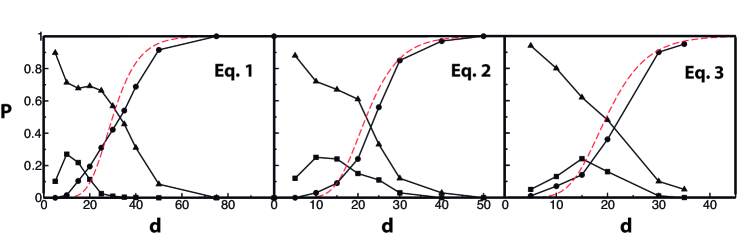
Figure 1: Numerically measured probability of different types of dynamics as a function of dimension $d$ of the phase space for Eq. (1) (left panel), Eq. (2) (central panel), Eq. (3) (right panel): $\bullet$ - chaotic trajectories, $\blacksquare$ - limit cycles, $\blacktriangle$ - stable fixed points. For each case, the theoretical estimate for the probability of chaotic trajectories (see main text) is shown by a dashed line (red color online).

Our main result is that for all considered types of non-linearity the probability of chaos increases with the dimension of the phase space, Fig. 1. In particular, the numerical simulations for (1,2,3) suggest that, essentially all trajectories become chaotic for $d\gtrsim 50$. Our simulations also indicate that already for intermediate dimensions $d\gtrsim 15$, the majority of chaotic trajectories essentially fill out the available phase space, i.e., become ergodic (Fig. 2, left panel). In such a regime the probability density $P(x_{i})$ for each coordinate of the chaotic attractor approaches a universal scaling form that depends neither on the choice of coefficients $\{a\},\{b\},\{c\}$ nor on the dimension $d$, Fig. 2. Furthermore, the LLEs also exhibits apparent scaling behavior, Fig. 3.

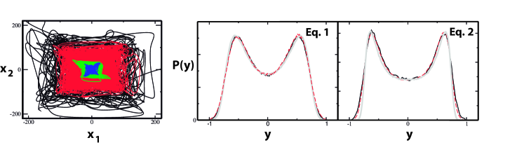
Figure 2: Scaling of the size of chaotic trajectories (color online). Left panel: Examples of $x_{1},x_{2}$ projections of trajectories for the dynamics described by (3) for $d=10$ (blue), $d=15$ (green), $d=30$ (red), and $d=45$(black), illustrating the scaling $x_{i}\sim d^{3/2}$. Central panel: The probability density for the scaled coordinate $P(y)$ vs. $y=x/d^{\alpha}$, $\alpha=1$ of the solution of Eq. (1) for $d=150$ (solid black line), $d=100$ (dashed red line), and the histogram of the solution of (10) (thick grey line). Right panel: The probability density for the scaled coordinate $P(y)$ vs. $y=x/d^{\alpha}$, $\alpha=3/4$ of the solution of Eq. (2) for $d=65$ (solid black line), $d=50$ (dashed red line), and the histogram of the solution of (10) (thick grey line).

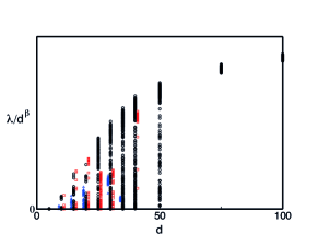
Figure 3: The scaled LLE $\lambda/d^{\beta}$ as a function of the dimension $d$ of phase space for (1); $\beta=2$, black circle; (2), $\beta=3$, square, shifted to the right, red online; and (3), triangle, shifted to the left, blue online, $\beta=9/2$. For large $d$, the LLE for (1) extrapolates to $\lambda/d^{\beta}\rightarrow\lambda^{*}\approx 0.235$ (see main text).

Below we explain the scaling and statistical properties of the large-$d$ limit of (1,2,3) First, consider the scaling of the spatial coordinates $x_{i}\sim d^{\alpha}$ and the LLEs $\lambda\sim d^{\beta}$ illustrated in Figs. 2 and 3. Consider the general case of a dynamical system similar to (1,2,3) with the $n$th-order highest nonlinear term and the $|x_{i}|^{m}\operatorname{sgn}(x_{i}),m>n$ diagonal confining term,

$$\frac{dx_{i}}{dt}=\sum_{k=1}^{n}\sum_{j_{1},\ldots,j_{k}=1}^{d}g_{i,j_{1},\ldots,j_{k}}^{(k)}x_{j_{1}}\ldots x_{j_{k}}-|x_{i}|^{m}\operatorname{sgn}(x_{i}).$$ (5)

Since the coefficients $g_{i,j_{1},\ldots,j_{k}}^{(k)}$ in (5) are drawn randomly, it is reasonable to assume that each coordinate has a similar scale, $x_{i}\sim x$ and (5) becomes

$$\frac{dx}{dt}\sim\sum_{k=1}^{n}x^{k}\sum_{j_{1},\ldots,j_{k}=1}^{d}g_{i,j_{1},\ldots,j_{k}}^{(k)}-|x|^{m}\operatorname{sgn}(x).$$ (6)

Here the $g_{i,j_{1},\ldots,j_{k}}^{(k)}$ are identically distributed random terms with zero mean and unit variance, and a typical value of the sum of $N$ such terms is the standard deviation $\sqrt{N}$, which yields the following scaling relation:

$$\frac{dx}{dt}\sim\sum_{k=1}^{n}x^{k}d^{k/2}-|x|^{m}\operatorname{sgn}(x).$$ (7)

Introducing new variables,

$$y =\frac{x}{d^{\alpha}},\;\alpha=\frac{n}{2(m-n)}$$ (8)

$$\theta =td^{\beta},\;\beta=\frac{n(m-1)}{2(m-n)}$$

we convert (7) into

$$\frac{dy}{d\theta}\sim\sum_{k=1}^{n}y^{k}d^{m(k-n)/[2(m-n)]}-|y|^{m}\operatorname{sgn}(y).$$ (9)

On the right-hand side of (9), the highest-order $k=n$ term and the $|y|\operatorname{sgn}(y)$ term do not depend on $d$ while the lower-order terms with $k<n$ vanish in the limit of $d\gg 1$. The transformation (8) explains the observed scaling of the size of chaotic attractors and the LLEs (whose dimension is the inverse of time) shown in Fig. 2 and 3. A more detailed example of the above derivation for Eq. (1) is given in id14. To explain the shape of the universal probability density $P(y)$ shown in Fig. 2, we ignore the irrelevant low-order terms and replace the leading nonlinear $n$th-order term (quadratic in (1) and cubic in (2,3)) by a stochastic function $f(\theta)$. This is done observing that for large $d$, the majority of the terms comprising the $\sum_{j_{1},\ldots,j_{n}=1}^{d}g_{i,j_{1},\ldots,j_{n}}^{(n)}$ do not contain $x_{i}$ and can be approximated as independent random variables. Since $\langle g^{2}\rangle=1$ by definition, it follows from the Central Limit theorem that this sum is a Gaussian random variable with variance $D=d^{n}\langle x^{2}\rangle^{n}$. This leads to the following approximation of (6) in the rescaled variables $y$ and $\theta$ of (8):

$$\frac{dy}{d\theta}=f(\theta)-y^{m},$$ (10)

where $f(\theta)$ is Gaussian process with dispersion $D$. To calculate the invariant measure of this process we approximate $f(t)$ by a jump process which takes constant Gaussian-distributed values $f_{i}$ during time intervals drawn from a uniform distribution with an average period $\tau$. We solve to the scaling equation (10) self-consistently, computing $\langle y^{2}\rangle^{n}$ from the histogram of the trajectory $y(\theta)$ produced via (10). Varying $\tau$, we find the best fit to the observed $P(y)$, which is shown as dashed lines in Fig. 2. Given the approximate nature of the temporal behaviour of $f(\theta)$ the fit seems quite satisfactory and yields $\tau^{(1)}=3.85$ for (1), $\tau^{(2)}=5.64$ for (2), and $\tau^{(3)}=6.63$ for (3) Note that the estimate for $\tau^{(1)}=3.85$ is in a qualitative agreement with the large-$d$ asymptotic value of the corresponding rescaled LLE $1/\lambda^{*}\approx 4.26$, (see Fig. 3), which characterizes the typical correlation time of the system.

Next we provide a statistical explanation for the probability of chaos as a function of the dimension $d$, as illustrated in  1. Consider stationary points of the dynamical systems (1,2,3). Since a system of $d$ $m$th-order algebraic equations generally has $md$ solutions (sometime coinciding), the dynamical system (1) has $md$ stationary points $x^{*}$. For our derivation, we assume that the system is chaotic if all these stationary points are unstable in at least one direction, i.e., if at each stationary point $x^{*}$ at least one eigenvalue of the local Jacobian matrix $J(x^{*})$ has a positive real part. We assume that for sufficiently high $d$, all Jacobian eigenvalues are statistically independent. This assumption of weakening correlations between dimensions as the number of dimensions increase is a rather strong approximation without which is seems impossible to derive analytical estimates, and which seems to result in reasonable results (see below). Denoting the probability that the real part of an eigenvalue is negative by $P_{neg}$, the probability that at least one out of $d$ eigenvalues of the Jacobian at a stationary point has a positive real part is $1-P_{neg}^{d}$. Hence the probability of chaos is

$$P_{chaos}=(1-P_{neg}^{d})^{md},$$ (11)

indicating that for any $P_{neg}=1-\epsilon<1$, the system becomes predominantly chaotic for $d\gtrsim 1/\epsilon$. Specifically, consider the example of system (2) with cubic non-linearities. If $x^{*}$ is a stationary point of (2), the elements of the Jacobian matrix $J(x^{*})=\left\{J_{ij}(x^{*})\right\}_{i,j=1}^{d}$ consist of two terms,

$$J_{ij}(x^{*}) =\sum_{k=1,l=1}^{d}(c_{ijkl}+c_{iljk}+c_{ilkj})x_{k}^{*}x_{l}^{*}-5x_{i}^{*4}\delta_{ij}$$ (12)

$$\equiv J_{ij}^{(1)}+J_{ij}^{(2)},$$

where $\left\{\delta_{ij}\right\}$ is the identity matrix. As above, we ignored low-order terms present in (5), because such terms are irrelevant for large $d$. We assume that the distribution of $x^{*}_{i}$ is the same as for the coordinates $x_{i}$ themselves and is given by the universal invariant measure shown in Fig. 2. We also consider the two terms $J_{ij}^{(1)}$ and $J_{ij}^{(2)}$ as statistically independent. The first term, $J_{ij}^{(1)}$, is a sum of $3d^{2}\gg 1$ random variables with zero mean and a finite variance. Taking into account that the dispersions of $c_{ijkl}$ are one, and $x_{i}$ and $\{c_{ijkl}\}$ are uncorrelated (this follows from the observed independence of $P(x)$ and the choice of $\{c\}$) the Central Limit theorem states that this sum is a Gaussian-distributed variable with zero mean and dispersion $\sigma^{2}=3d^{2}\langle x^{2}\rangle^{2}$. It follows from “Girko’s circular law” girko1984 that eigenvalues of a random $d\times d$-matrix with Gaussian-distributed elements with zero mean and unit variance are uniformly distributed on a disk in the complex plane with radius $\sqrt{d}$. Thus, the eigenvalues of $J_{ij}^{(1)}$ are uniformly distributed on a disk with radius $\sigma\sqrt{d}$. The probability for an eigenvalue of $J_{ij}^{(1)}$ to have real part $r\sigma\sqrt{d}$, with $|r|\leq 1$, is then proportional to the length of the chord intersecting the radius of the disk at the point $r$,

$$P_{c}(r)=\frac{2\sqrt{1-r^{2}}}{\pi}.$$ (13)

(The factor $2/\pi$ normalizes $P_{c}(r)$ to one.) The probability distribution of the second, diagonal, term of the Jacobian, $J_{ij}^{(2)}=-5x_{i}^{*4}\delta_{ij}$ is defined by the invariant measure $P(y)$, given by (10) and shown in Fig. 2. It follows from scaling (8) that both $J_{ij}^{(1)}$ and $J_{ij}^{(2)}$ contribute terms of order $d^{3}$ to the eigenvalues of the Jacobian. The contribution from $J_{ij}^{(1)}$ may have a positive or a negative real part with equal probability $1/2$. The contribution from $J_{ij}^{(2)}$ is always negative and has magnitude $5y^{4}$ with probability $P(y)$. It follows that the probability that the sum of the two contributions has negative real part is

$$P_{neg}=\frac{1}{2}+\int\limits_{-\infty}^{+\infty}P(y)dy\int\limits_{0}^{5y^{4}/\chi}P_{c}(r)dr.$$ (14)

where $\chi\equiv\sigma/d^{5/2}=\sqrt{3}\langle y^{2}\rangle$. Integration on $dr$ produces

$$P_{neg}=\frac{1}{2}\left[1+\int\limits_{|y|>(\chi/5)^{1/4}}P(y)dy\right]$$ (15)

$$+\int\limits_{|y|<(\chi/5)^{1/4}}\frac{\sin^{-1}(5y^{4}/\chi)+5y^{4}/\chi\sqrt{1-(5y^{4}/\chi)^{2}}}{\pi}P(y)dy.$$

Using the numerical data for $P(y)$ shown in Fig. 2 we calculate $\chi\approx 0.446$ and perform numerical integration of $P(y)$ to obtain $P_{neg}^{(2)}\approx 0.794$. A similar analysis for Eqs. (1) (id14) and (3) yields $P_{neg}^{(1)}\approx 0.849$ and $P_{neg}^{(3)}\approx 0.787$, respectively. Substituting these values into Eq. (11) provides a reasonable fit for the observed probability of chaos, as illustrated by the dashed lines in  1. An increasing discrepancy for lower $d$ could be attributed to the facts that the systems reach truly scaling regime for $d\rightarrow\infty$ and the histograms in Fig. 2 are measured for rather high $d\geq 45$.

To summarize, we have presented numerical evidence that the behaviour of generic dissipative dynamical systems in continuous time universally becomes chaotic and ergodic as the dimension of the phase space becomes large ($d\sim 50$ in the three cases we studied). We note that the quadratic and cubic non-linearities considered here can be interpreted as the first few non-linear terms in the expansion of more complex non-linear dynamical systems, possibly extending the applicability of our results. We have also provided some analytical explanations for the observed ubiquity of chaos and for the universality of the density distribution of chaotic trajectories. The similarity of the three panels in Fig. 1 and the apparently general applicability of Eq. (11) suggest that the observed transition to chaos is not limited to the three cases considered here and instead universally occurs in all high-dimensional nonlinear dissipative dynamical systems. One of the goals of this work was to illustrate the transition to chaos and ergodicity in high-dimensional phase space, a frequently used yet rarely precisely stated argument in the formal justification of statistical mechanics. Nevertheless, to explain our results we use scaling and probabilistic arguments borrowed from statistical physics. Thus, our results are an attempt to use statistical physics to establish a basic “phase diagram” of dynamical systems.

Acknowledgement I.I. was supported by FONDECYT 1110288. M.D. was supported by NSERC, Canada. S. A. acknowledges financial support from FONDECYT 11121214 and 1120356, Grant ICM P10-061-F by FIC-MINECON, Financiamiento Basal para Centros Científicos y Tecnológicos de Excelencia FB 0807, and Concurso Inserción en la Academia-Folio 791220017.