The G+M eclipsing binary V530 Orionis: A stringent test of magnetic stellar evolution models for low-mass stars

Abstract

We report extensive photometric and spectroscopic observations of the 6.1-day period, G+M-type detached double-lined eclipsing binary V530 Ori, an important new benchmark system for testing stellar evolution models for low-mass stars. We determine accurate masses and radii for the components with errors of 0.7% and 1.3%, as follows: $M_{\rm A}=1.0038\pm 0.0066$ $M_{\sun}$, $M_{\rm B}=0.5955\pm 0.0022$ $M_{\sun}$, $R_{\rm A}=0.980\pm 0.013$ $R_{\sun}$, and $R_{\rm B}=0.5873\pm 0.0067$ $R_{\sun}$. The effective temperatures are $5890\pm 100$ K (G1 V) and $3880\pm 120$ K (M1 V), respectively. A detailed chemical analysis probing more than 20 elements in the primary spectrum shows the system to have a slightly subsolar abundance, with ${\rm[Fe/H]}=-0.12\pm 0.08$. A comparison with theory reveals that standard models underpredict the radius and overpredict the temperature of the secondary, as has been found previously for other M dwarfs. On the other hand, models from the Dartmouth series incorporating magnetic fields are able to match the observations of the secondary star at the same age as the primary ($\sim$3 Gyr) with a surface field strength of $2.1\pm 0.4$ kG when using a rotational dynamo prescription, or $1.3\pm 0.4$ kG with a turbulent dynamo approach, not far from our empirical estimate for this star of $0.83\pm 0.65$ kG. The observations are most consistent with magnetic fields playing only a small role in changing the global properties of the primary. The V530 Ori system thus provides an important demonstration that recent advances in modeling appear to be on the right track to explain the long-standing problem of radius inflation and temperature suppression in low-mass stars.

1. Introduction

The discovery of V530 Ori (HD 294598, BD$-$03 1283, 2MASS J06043380$-$0311513) as an eclipsing binary was made by Strohmeier (1959), who established an orbital period for the system of 6.110792 days. The depth reported for the primary eclipse was about 0.7 mag, but no secondary eclipse was seen in these early photographic measurements. The primary star is of solar type. The object has received little attention following the discovery, other than the occasional measurement of times of primary eclipse, which was the only eclipse detected until recently. It was claimed by Sahade & Berón Dávila (1963) to be a possible member of the Collinder 70 cluster, a proposal that appears to have since been dismissed. Faint spectral lines of the secondary with about the same width as those of the primary were first detected in 1985 by Lacy (1990), but remained elusive in subsequent high-resolution observations (see, e.g. Popper, 1996). Similarly, no signs of the secondary eclipse could be seen in more recent photometric monitoring, implying either a very faint and cool companion, or possibly an eccentric orbit and a special orientation such that no secondary eclipses occur.

This motivated us to begin our own program of spectroscopic observation in 1996. Our interest in the system was piqued when we were able to derive the first single-lined spectroscopic orbit, which is indeed eccentric but only slightly so, and to predict the exact location of the secondary eclipse, which we were then successful in detecting with more targeted photometric observations. The depth in $V$ is less than 3%. Continued analysis has enabled us to also measure radial velocities for the secondary, and to fully characterize the binary.

The confirmed presence of a late-type star in V530 Ori makes it a rare example of a system containing a solar-type primary that is easy to study and provides access to other key properties of the binary, and at the same time a late-type secondary that is very faint but still measurable. As such, V530 Ori is potentially very useful for testing models of stellar evolution if accurate properties for the stars can be derived, by virtue of the greater leverage afforded by a mass ratio significantly different from unity. Previous measurements for M dwarfs have shown rather serious disagreements with models in the sense that such stars appear larger and cooler than predicted by theory (e.g., Torres & Ribas, 2002; Ribas, 2003; López Morales & Ribas, 2005; Torres, 2013). This is now widely believed to be related to stellar activity (magnetic inhibition of convection, and/or star spots; Mullan & MacDonald, 2001; Chabrier et al., 2007; Feiden & Chaboyer, 2012), but there are relatively few systems containing M stars with complete information available for testing this hypothesis.

Here we provide a full description of our spectroscopic and photometric observations of V530 Ori, leading to the first determination of accurate properties for the stars including the absolute masses and radii. We report also a detailed chemical analysis of the system based on the solar-type primary star, bypassing the usual difficulties and limitations of determining the metallicity of M stars. We additionally estimate the surface magnetic field strengths for both components, an important piece of information permitting a more meaningful comparison with recent models that incorporate magnetic fields. Our results provide one of the clearest illustrations that such models are indeed able to reproduce the measured properties of low-mass stars.

2. Ephemeris

Dates of minimum light for V530 Ori were collected from the literature and from our own unpublished photometric measurements (see Table 1), and were used to establish the ephemeris. The measurements (34 timings for the primary and 7 for the secondary) span about 82 years, or $\sim$4900 orbital cycles of the binary. Uncertainties for the older timings and for some of the more recent ones have not been published, so we determined them by iterations to achieve reduced $\chi^{2}$ values near unity, separately for each type of measurement ($\sigma=0.028$, 0.011, and 0.0001 days for the photographic, visual, and photoelectric/CCD data). We found we also needed to rescale the published photoelectric/CCD errors by factors of 1.8 and 2.9 for the primary and secondary, respectively. A linear weighted least-squares fit using the primary and secondary minima together resulted in

$${\rm Min~{}I~{}(HJD)}=2,\!453,\!050.826061(91)+6.11077840(33)E$$

$${\rm Min~{}II~{}(HJD)}=2,\!453,\!053.6623(16)+6.11077840(33)E\,,$$

which we have used in the analysis that follows. Uncertainties are indicated in parentheses in units of the last significant digit.

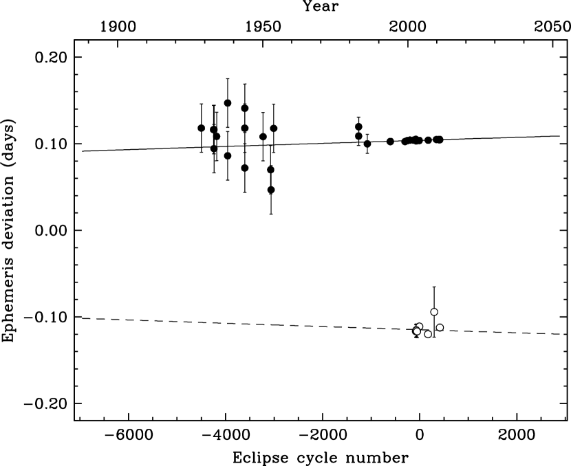
Figure 1.— Ephemeris curve for V530 Ori from the fit described in the text. Times of eclipse are shown with filled circles for the primary and open circles for the secondary. Eclipse cycles are counted from the reference epoch given in the text. The corresponding apsidal period is $U=7800\pm 22000$ years.

Secondary eclipses occur at a phase of $0.46414(27)$, clearly showing that the orbit is eccentric. Some degree of apsidal motion is therefore expected. An ephemeris curve (Lacy, 1992a) was fit to all the data with the same weighting scheme as above, adopting values for the eccentricity and inclination angle derived in our spectroscopic and light curve analyses below, and is illustrated in Figure 1. However, the apsidal period is only poorly determined from this fit ($U=7800\pm 22000$ years).

Table 1Times of eclipse for V530 Ori.

	HJD	$\sigma$			$(O-C)$
Year	(2,400,000$+$)	(days)	Epoch	Ecl	(days)	Type	Source
1928.8527	25558.456	$\cdots$	$-$4499	1	$+$0.0220	PG	1
1933.0688	27098.370	$\cdots$	$-$4247	1	$+$0.0198	PG	1
1933.2193	27153.345	$\cdots$	$-$4238	1	$-$0.0022	PG	1
1933.2193	27153.367	$\cdots$	$-$4238	1	$+$0.0198	PG	1
1934.1228	27483.341	$\cdots$	$-$4184	1	$+$0.0118	PG	1

Note. — This table is available in its entirety in machine-readable and Virtual Observatory (VO) forms in the online journal. A portion is shown here for guidance regarding its form and content.

3. Spectroscopic observations

V530 Ori was monitored spectroscopically with three different instruments over a period of more than 17 years. Observations began at the Harvard-Smithsonian Center for Astrophysics (CfA) in 1996 June with a Cassegrain-mounted echelle spectrograph (“Digital Speedometer” (DS); Latham, 1992) attached to the 1.5 m Tillinghast reflector at the F. L. Whipple Observatory (Mount Hopkins, AZ). Those observations continued through 2009 April. The spectra consist of a single order 45 Å wide recorded with an intensified photon-counting Reticon detector at a central wavelength of 5187 Å, which includes the Mg I b triplet. The resolving power provided by this setup is $R\approx 35,\!000$. Additional observations were collected with a nearly identical instrument attached to the 4.5 m-equivalent Multiple Mirror Telescope (also on Mount Hopkins), prior to its conversion to a monolithic 6.5 m telescope. The 74 usable spectra from these instruments have signal-to-noise ratios (SNRs) ranging from about 10 to 50 per resolution element of 8.5 km s^-1. Observations of the dusk and dawn sky were made every night to monitor the velocity zero point, and to establish small run-to-run corrections applied to the DS velocities reported below.

We gathered a further 30 spectra of V530 Ori at the Kitt Peak National Observatory (KPNO) from 1999 March to 2001 January, using the coudé-feed telescope and the coudé spectrometer. The spectra cover the wavelength region 6450–6600 Å, and include the H$\alpha$ line. The 250 $\mu$m slit and OG 550 filter projected onto 0.186 Å on the detector. The detector was a Ford $3072\times 1024$ pixel CCD (F3KB) with 15 $\mu$m square pixels. The ‘A’ grating (632 grooves mm^-1) was used in the second order with Camera 5 (a folded Schmidt design). The spectra were flat-fielded and wavelength calibrated following standard procedures, based on quartz lamp flats and Th-Ar emission tube spectra. Observations of the standard stars $\iota$ Psc or $\beta$ Vir were taken with the same setup during the same nights in order to correct for instrumental drifts. The adjustments assumed constant velocities of $+5.636$ km s^-1 for $\iota$ Psc (HD 222368) and $+4.468$ km s^-1 for $\beta$ Vir (HD 102870), from Nidever et al. (2002).

Finally, 41 additional observations were obtained at the CfA from 2009 November to 2014 March with the Tillinghast Reflector Echelle Spectrograph (TRES; Fűrész, 2008) on the 1.5 m telescope mentioned earlier. This bench-mounted instrument yields a resolving power of $R\approx 44,\!000$, and spectra spanning 3860–9100 Å in 51 orders. The SNRs range from 13 to 121 per resolution element of 6.8 km s^-1. Instrumental drifts for TRES are below 10 m s^-1 in velocity, which is negligible for our purposes.

Lines of the very faint secondary star in V530 Ori are not immediately obvious in any of our spectra, even in the redder ones from KPNO, but its radial velocities (RVs) can nevertheless be measured accurately along with those of the primary using the two-dimensional cross-correlation algorithm TODCOR (Zucker & Mazeh, 1994). Templates for the DS and TRES spectra were selected from a large library of calculated spectra based on model atmospheres by R. L. Kurucz (see Nordström et al., 1994; Latham et al., 2002) and a line list prepared by J. Morse. These templates cover approximately 300 Å centered on the Mg I b region, and include numerous other lines mainly of Fe, Ca, and Ti. For the KPNO spectra we used a different template library based on PHOENIX models (see Husser et al., 2013), kindly computed for us by I. Czekala for the wavelength region of interest. Our synthetic templates are parametrized in terms of the effective temperature ($T_{\rm eff}$), rotational velocity ($v\sin i$ when seen in projection), surface gravity ($\log g$), and metallicity, ${\rm[Fe/H]}$. The latter two have a minimal impact on the velocities, so we adopted fixed values of $\log g=4.5$ and solar composition for both stars. The optimum template parameters ($T_{\rm eff}$ and $v\sin i$) for the primary were determined following Torres et al. (2002) by running grids of cross-correlations seeking the best template match as measured by the mean cross-correlation coefficient averaged over all exposures. This was done separately for the three sets of spectra, with very consistent results. We obtained $T_{\rm eff}=6000$ K and $v\sin i=10$ km s^-1. The faintness of the secondary, which has a flux some 40 times smaller than that of the primary, prevents us from determining its template parameters in a similar way. Instead we relied on the temperature difference inferred from our light curve solutions in Sect. 6, and we assumed the star is rotating synchronously. The latter is a reasonable assumption, as the timescale for synchronization of the secondary ($\sim$10⁷ yr; see, e.g., Hilditch, 2001) is much shorter than the $\sim$3 Gyr age we estimate for the system later in Sect. 8. With these constraints the template parameters for the secondary were $T_{\rm eff}=4000$ K and $v\sin i=6$ km s^-1.

The final heliocentric velocities from the TRES spectra are the average of the measurements from the three echelle orders covered by the templates, and are listed in Table 2. Typical uncertainties are 0.05 km s^-1 for the primary (star A) and 1.6 km s^-1 for the faint secondary (star B). Experience has shown that the very narrow wavelength range of the DS spectra (45 Å) can sometimes lead to systematic errors in the RVs due to residual line blending as well as lines shifting in and out of the spectral window as a function of orbital phase (see Latham et al., 1996). We investigated this by means of numerical simulations for each spectrum, and found the effect to be significant (shifts of up to 7 km s^-1 for the secondary, but only 0.02 km s^-1 for the primary). We therefore applied corrections to the individual velocities in the same way as done in previous studies with similar spectroscopic material (e.g., Torres et al., 1997; Lacy et al., 2010) in order to remove the bias. These adjustments increase the minimum masses by about 4% for the primary star and 2% for the secondary. The final DS velocities with corrections included are given also in Table 2. They have typical uncertainties of 0.5 km s^-1 and 6.7 km s^-1 for the primary and secondary, respectively. RVs from the KPNO observations are based on the entire wavelength range of those spectra except for the broad H$\alpha$ line, which was masked out. Those measurements (two being excluded here for giving very large residuals from the orbit described in the next section) are presented with the others in Table 2. Their uncertainties are typically 0.4 km s^-1 for the primary and 5.4 km s^-1 for the secondary.

Table 2Heliocentric radial velocity measurements of V530 Ori.

HJD	Orbital	$RV_{\rm A}$	$RV_{\rm B}$	$(O-C)_{\rm A}$	$(O-C)_{\rm B}$
(2,400,000$+$)	phase	(km s-1)	(km s-1)	(km s-1)	(km s-1)	Instrument
50407.0052	0.3513	$-$68.18	28.42	$-$0.41	$+$5.33	DS
50412.8283	0.3042	$-$78.55	43.26	$-$0.38	$+$2.63	DS
50441.8571	0.0546	$-$57.79	1.31	$-$1.05	$-$3.19	DS
50448.7155	0.1770	$-$86.70	58.24	$-$0.65	$+$4.33	DS
50474.7700	0.4406	$-$43.10	$-$17.49	$+$0.38	$+$0.35	DS

Note. — This table is available in its entirety in machine-readable and Virtual Observatory (VO) forms in the online journal. A portion is shown here for guidance regarding its form and content.

Our TODCOR analyses also provided an estimate of the light ratio between the primary and secondary at the mean wavelength of our spectra (see Zucker & Mazeh, 1994). For the DS observations we obtained $\ell_{\rm B}/\ell_{\rm A}=0.014\pm 0.002$ in the Mg I b region, corresponding to a magnitude difference $\Delta m=4.6$. The TRES spectra yielded a similar value of $0.013\pm 0.002$ for the average of the three orders used to measure RVs, centered also on the Mg I b region. As expected from the spectral types, the secondary appears brighter at the redder wavelengths of the KPNO spectra, and the light ratio obtained there is $0.042\pm 0.003$ at a mean wavelength of 6410 Å.

Our TRES spectra display moderately strong emission cores in the Ca II H and K lines, which is indicative of stellar activity. Measurement of the radial velocity of the emission cores shows that they follow the center of mass of the primary, and are thus associated with that star. Further evidence of activity is presented below.

3.1. Spectroscopic orbital solution

Separate spectroscopic orbital solutions using the three velocity data sets were carried out to check for potential systematic differences, with the ephemeris held fixed at the values in Sect. 2. The results shown in Table 3 indicate fairly good agreement considering the faintness of the secondary and the difficulty in measuring its velocity. Our adopted solution combining all of the RVs is given in the last column, where we have allowed for arbitrary offsets between the DS and KPNO velocities relative to those measured with TRES, which are non-negligible in both cases. The TRES velocities dominate because of their considerably smaller uncertainties; the rms residuals ($\sigma_{\rm A}$ and $\sigma_{\rm B}$) are listed at the bottom of the table along with other quantities of interest. We find the orbit to be slightly eccentric ($e=0.08802\pm 0.00023$), consistent with predictions from theory for this system indicating a timescale for tidal circularization of $\sim$18 Gyr (e.g., Hilditch, 2001).

Table 3Spectroscopic orbital solutions for V530 Ori.

Parameter	TRES	DS	KPNO	Combined
$P$ (days)	6.11077840 (fixed)	6.11077840 (fixed)	6.11077840 (fixed)	6.11077840 (fixed)
$\gamma$ (km s-1)	$-$33.529 $\pm$ 0.0110+	$-$33.901 $\pm$ 0.0700+	$-$32.931 $\pm$ 0.0790+	string$-$33.525 $\pm$ 0.0110+
$K_{\rm A}$ (km s-1)	50.9057 $\pm$ 0.00830	50.986 $\pm$ 0.0600	50.96 $\pm$ 0.100	50.9075 $\pm$ 0.00800
$K_{\rm B}$ (km s-1)	85.73 $\pm$ 0.270	87.12 $\pm$ 0.850	84.8 $\pm$ 1.40	85.81 $\pm$ 0.250
$e$	0.08791 $\pm$ 0.00024	0.0895 $\pm$ 0.0012	0.0903 $\pm$ 0.0019	0.08802 $\pm$ 0.00023
$\omega_{\rm A}$ (deg)	129.33 $\pm$ 0.1700	129.2 $\pm$ 1.100	129.5 $\pm$ 1.000	129.35 $\pm$ 0.1600
$T$ (HJD$-$2,400,000)	53050.826061 (fixed)	53050.826061 (fixed)	53050.826061 (fixed)	53050.826061 (fixed)
$\Delta RV$(TRES$-$DS) (km s-1)	$\cdots$	$\cdots$	$\cdots$	$+$0.413 $\pm$ 0.055+
$\Delta RV$(TRES$-$KPNO) (km s-1)	$\cdots$	$\cdots$	$\cdots$	$-$0.596 $\pm$ 0.080+
Derived quantities
$M_{\rm A}\sin^{3}i$ (M☉)	1.0016 $\pm$ 0.0071	1.040 $\pm$ 0.023	0.978 $\pm$ 0.035	1.0038 $\pm$ 0.0066
$M_{\rm B}\sin^{3}i$ (M☉)	0.5948 $\pm$ 0.0024	0.6084 $\pm$ 0.0076	0.588 $\pm$ 0.012	0.5955 $\pm$ 0.0022
$q\equiv M_{\rm B}/M_{\rm A}$	0.5938 $\pm$ 0.0019	0.5852 $\pm$ 0.0058	0.6009 $\pm$ 0.0097	0.5932 $\pm$ 0.0017
$a_{\rm A}\sin i$ ($10^{6}$ km)	4.26101 $\pm$ 0.00069	4.2671 $\pm$ 0.0051	4.2649 $\pm$ 0.0087	4.26112 $\pm$ 0.00067
$a_{\rm B}\sin i$ ($10^{6}$ km)	7.176 $\pm$ 0.023	7.291 $\pm$ 0.071	7.10 $\pm$ 0.11	7.183 $\pm$ 0.021
$a\sin i$ (R☉)	16.440 $\pm$ 0.0330	16.62 $\pm$ 0.100	16.33 $\pm$ 0.160	16.450 $\pm$ 0.0300
Other quantities pertaining to the fit
$N_{\rm A}$ , $N_{\rm B}$, TRES	41 , 41	$\cdots$	$\cdots$	41 , 41
$N_{\rm A}$ , $N_{\rm B}$, DS	$\cdots$	74 , 74	$\cdots$	74 , 74
$N_{\rm A}$ , $N_{\rm B}$, KPNO	$\cdots$	$\cdots$	28 , 28	28 , 28
Time span (days)	1585.8	4521.6	663.2	6323.7
$\sigma_{\rm A}$ , $\sigma_{\rm B}$, TRES (km s-1)	0.049 , 1.66	$\cdots$	$\cdots$	0.048 , 1.63
$\sigma_{\rm A}$ , $\sigma_{\rm B}$, DS (km s-1)	$\cdots$	0.46 , 6.65	$\cdots$	0.47 , 6.70
$\sigma_{\rm A}$ , $\sigma_{\rm B}$, KPNO (km s-1)	$\cdots$	$\cdots$	0.42 , 5.47	0.42 , 5.37

A graphical representation of our fit appears in Figure 2 together with the observations and the RV residuals, the latter shown separately for each data set.

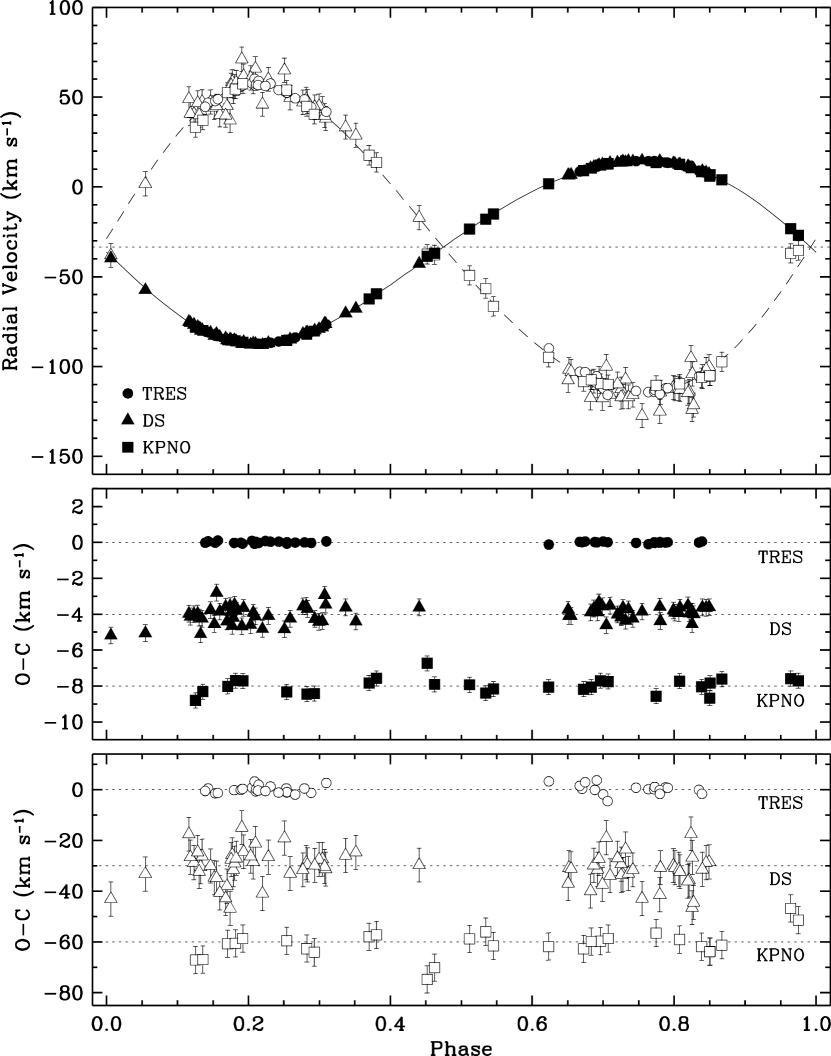
Figure 2.— Top: Radial velocities for V530 Ori and our model from the combined solution of Table 3 (solid line for the primary, dashed for the secondary). The dotted line marks the center-of-mass velocity of the system, and phase 0.0 corresponds to primary eclipse. Measurements from different data sets are represented with different symbols, as labeled. Middle: Velocity residuals ($O-C$) for the primary star, shown separately for each data set. The DS and KPNO residuals are displaced vertically for clarity. Bottom: Same as middle panel, for the secondary.

3.2. Spectral disentangling

Although a number of eclipsing binaries containing M stars have been studied in the past, in very few cases is the metallicity of the system known because of the difficulty of analyzing the spectra of late-type stars, which are dominated by strong molecular features. In V530 Ori the primary is a solar-type star, for which an abundance analysis would be straightforward except for the fact that its spectrum is contaminated at some level by the secondary. To remove this effect we have subjected our observations to spectral disentangling (Bagnuolo & Gies, 1991; Simon & Sturm, 1994; Hadrava, 1995), by which we are able to reconstruct the spectra of the individual components for further analysis. Pavlovski & Hensberge (2005) and others have shown that disentangled spectra can yield reliable abundances (see also Pavlovski & Hensberge, 2010; Pavlovski & Southworth, 2012).

The application of the technique to V530 Ori pushes it to the limit because of the extreme faintness of the secondary (2.5% fractional light in $V$, and even less toward the blue) and the modest SNRs of our spectra. Some previous studies have succeeded in similar situations with light ratios of $\sim$5% (e.g., Pavlovski et al., 2009; Lehman et al., 2013; Tkachenko et al., 2014) and even 1.5–2% (Holmgren et al., 1999; Pavlovski et al., 2010; Mayer et al., 2013), but with spectra of considerably higher SNR than ours.

We performed disentangling separately for each of our three data sets (TRES, DS, KPNO) because of their different spectral resolutions and wavelength coverage, discarding a few spectra with low SNR. We used the program FDBinary (Ilijić et al., 2004), which implements disentangling in the Fourier domain (Hadrava, 1995). For the DS and KPNO observations we disentangled the entire spectral range available, and for TRES we restricted ourselves to the interval 4475–6760 Å to avoid regions with lower flux or telluric contamination. Special care was taken to select spectral stretches with both ends in the continuum, as required by the algorithm. Given the the rich line spectrum the wavelength regions we disentangled differ in length from 30 Å to 150 Å. Renormalization of the disentangled spectra (see Pavlovski & Hensberge, 2005; Lehman et al., 2013) was performed using the measured light ratios reported earlier from our spectroscopic analysis as well as those below from our light curve fits, interpolating or extrapolating linearly as needed.

The disentangled spectrum of the primary star gains in SNR compared to the individual spectra roughly as ${\rm SNR_{A}}\sim\langle{\rm SNR}\rangle\sqrt{N}/(1+\ell_{\rm B}/\ell_{\rm A})$, where $N$ is the number of spectra and $\langle{\rm SNR}\rangle$ the average SNR of the individual spectra. A similar expression holds for the disentangled secondary spectrum, with the light ratio reversed. The spectra resulting from the procedure have SNRs of 246 (primary) and 8 (secondary) for TRES ($\lambda$5800, $N=27$), 103 and 1.4 for DS ($\lambda$5200, $N=67$), and 713 and 30 for KPNO ($\lambda$6400, $N=30$). Portions of the disentangled TRES spectra appear in Figure 3, where a comparison with a model in the bottom panel shows that the secondary spectrum was successfully reconstructed from these observations, despite its faintness.

Figure 3.— Top: Sample sections of the disentangled spectra of the primary and secondary of V530 Ori from our TRES observations. Bottom: Disentangled spectrum of the secondary (bottom) in a region containing strong Ca I lines, compared to a synthetic spectrum (top) with parameters $T_{\rm eff}=3900$ K, $\log g=4.65$, and $v\sin i=5$ km s^-1, close to those appropriate for the star. The model spectrum has been scaled to a light ratio of 4% relative to the primary.

4. Chemical abundance

We subjected the disentangled spectra of the primary component to a detailed analysis to determine the effective temperature and chemical abundance. A first estimate of $T_{\rm eff}$ was made by fitting the Balmer line profiles, which depend primarily on temperature and very little on $\log g$, via genetic minimization (Tamajo et al., 2011). Metal lines in the wings were masked out, and the surface gravity and $v\sin i$ were held fixed at values reported below in Sect. 7. We obtained temperatures of $5840\pm 50$ K and $5870\pm 45$ K from H$\alpha$ and H$\beta$ in the TRES spectra, and $5780\pm 55$ K from H$\alpha$ in the KPNO spectra. These uncertainties may be underestimated, however, as we cannot rule out systematics from the normalization process and merging of the echelle orders.

We then used the uclsyn package (Smalley et al., 2011) to fine-tune the temperature and set the microturbulent velocity $\xi_{\rm t}$ from the numerous Fe I lines, and to determine the detailed abundances based on the measured equivalent widths. Surface gravity was held fixed as above. uclsyn relies on synthetic spectra computed under local thermodynamic equilibrium (LTE) using ATLAS9 model atmospheres (Kurucz, 1979). Excitation equilibrium was imposed to determine $T_{\rm eff}$ from the Fe I lines, with the selection of lines and their $gf$ values taken from the recent critical compilation of Bensby et al. (2014). Microturbulence was determined by enforcing no dependence between the abundances and the reduced equivalent widths. We obtained $T_{\rm eff}=5890\pm 80$ K and $\xi_{\rm t}=1.2\pm 0.1$ km s^-1 from the TRES spectra, and $T_{\rm eff}=5970\pm 110$ K and $\xi_{\rm t}=1.7\pm 0.1$ km s^-1 from the red KPNO spectra. We attribute the discrepancy in $\xi_{\rm t}$ values to the greatly different wavelength coverage of the TRES and KPNO spectra. The DS spectra do not permit independent estimates of these parameters because of the very limited wavelength coverage, so they were fixed at values of 5900 K and 1.2 km s^-1. We collect the various temperature determinations for the primary star in Table 4, along with others described later, noting that they are not all completely independent as some of them rely on the same sets of spectra.

Table 4Effective temperature estimates for V530 Ori A.

Method	$T_{\rm eff}$ (K)
TRES spectra, H$\alpha$	$5840\pm 50$0
TRES spectra, H$\beta$	$5870\pm 45$0
KPNO spectra, H$\alpha$	$5780\pm 55$0
TRES spectra, uclsyn	$5890\pm 80$0
KPNO spectra, uclsyn	$5970\pm 110$
DS spectra, cross-correlation	$5880\pm 100$
TRES spectra, cross-correlation	$5880\pm 100$
KPNO spectra, cross-correlation	$5820\pm 100$
Color indices and $J_{\rm B}$	$5950\pm 30$0

Note. — Uncertainties are formal errors, and may not reflect systematics.

Detailed abundances on the scale of Asplund et al. (2009) were obtained for 21 species from the TRES spectra, as listed in Table 5, and somewhat fewer for the DS and KPNO spectra. The uncertainties account for errors in $T_{\rm eff}$ and $\xi_{\rm t}$ of 100 K and 0.1 km s^-1, respectively. The agreement between the three instruments is excellent, the average differences for all elements taken together being $\langle{\rm TRES}-{\rm DS}\rangle=+0.022\pm 0.014$ dex (10 lines in common), $\langle{\rm TRES}-{\rm KPNO}\rangle=-0.011\pm 0.032$ dex (7 lines), and $\langle{\rm DS}-{\rm KPNO}\rangle=-0.022\pm 0.029$ dex (4 lines). In particular, the iron abundances based on Fe I are very consistent. Those from Fe II are somewhat less reliable and are based on far fewer lines. We adopted the weighted average of the Fe I values, ${\rm[Fe/H]}=-0.12\pm 0.08$, with a conservative uncertainty. Abundances of most other elements in V530 Ori tend to be subsolar as well. This includes the $\alpha$ elements, which are therefore not enhanced in this system.

Table 5V530 Ori abundances from our disentangled TRES, DS, and KPNO spectra.

			TRES			DS			KPNO
A	Elem		$N$	[X/H]		$N$	[X/H]		$N$	[X/H]		$\log\epsilon_{\sun}$
6	C I		4	$+0.06\pm 0.10$		$\cdots$	$\cdots$		$\cdots$	$\cdots$		$8.43\pm 0.05$
11	Na I		5	$-0.07\pm 0.09$		$\cdots$	$\cdots$		$\cdots$	$\cdots$		$6.24\pm 0.04$
12	Mg I		9	$-0.16\pm 0.07$		3	$-0.24\pm 0.09$		3	$-0.29\pm 0.06$		$7.60\pm 0.04$
13	Al I		4	$-0.06\pm 0.08$		$\cdots$	$\cdots$		$\cdots$	$\cdots$		$6.45\pm 0.03$
14	Si I		15	$-0.11\pm 0.04$		$\cdots$	$\cdots$		10	$-0.04\pm 0.06$		$7.51\pm 0.03$
16	S I		5	$+0.02\pm 0.10$		$\cdots$	$\cdots$		$\cdots$	$\cdots$		$7.12\pm 0.03$
20	Ca I		21	$-0.03\pm 0.10$		$\cdots$	$\cdots$		9	$-0.11\pm 0.09$		$6.34\pm 0.04$
21	Sc II		12	$-0.11\pm 0.06$		$\cdots$	$\cdots$		$\cdots$	$\cdots$		$3.15\pm 0.04$
22	Ti I		32	$-0.10\pm 0.10$		5	$-0.12\pm 0.12$		$\cdots$	$\cdots$		$4.95\pm 0.05$
23	V I		28	$+0.04\pm 0.11$		4	$+0.07\pm 0.12$		$\cdots$	$\cdots$		$3.93\pm 0.08$
24	Cr I		15	$-0.12\pm 0.09$		19	$-0.07\pm 0.07$		2	$-0.05\pm 0.08$		$5.64\pm 0.04$
25	Mn I		19	$-0.09\pm 0.09$		2	$-0.14\pm 0.13$		$\cdots$	$\cdots$		$5.43\pm 0.05$
26	Fe I		132	$-0.11\pm 0.06$		38	$-0.14\pm 0.09$		41	$-0.11\pm 0.07$		$7.50\pm 0.04$
26	Fe II		23	$-0.16\pm 0.08$		$\cdots$	$\cdots$		4	$-0.07\pm 0.06$		$7.50\pm 0.04$
27	Co I		11	$-0.12\pm 0.09$		7	$-0.18\pm 0.09$		$\cdots$	$\cdots$		$4.99\pm 0.07$
28	Ni I		48	$-0.13\pm 0.09$		13	$-0.16\pm 0.10$		12	$-0.07\pm 0.06$		$6.22\pm 0.04$
29	Cu I		4	$-0.15\pm 0.06$		$\cdots$	$\cdots$		$\cdots$	$\cdots$		$4.19\pm 0.04$
30	Zn I		3	$-0.23\pm 0.09$		$\cdots$	$\cdots$		$\cdots$	$\cdots$		$4.56\pm 0.05$
39	Y II		10	$-0.28\pm 0.07$		3	$-0.34\pm 0.10$		$\cdots$	$\cdots$		$2.21\pm 0.05$
56	Ba II		5	$-0.18\pm 0.12$		$\cdots$	$\cdots$		$\cdots$	$\cdots$		$2.18\pm 0.09$
60	Nd II		10	$-0.03\pm 0.06$		4	$+0.00\pm 0.07$		$\cdots$	$\cdots$		$1.42\pm 0.04$

Note. — Columns list the atomic number, the element and ionization degree, the number of spectral lines measured and abundance relative to the Sun from each instrument, and finally the reference photospheric solar values from Asplund et al. (2009). Abundances of other elements based on a single line are considered less reliable and are not listed.

5. Photometric observations

Two sets of $V$-band images of V530 Ori were obtained with independent robotic telescopes operating at the University of Arkansas (URSA WebScope) and near Silver City, NM (NFO WebScope) from 2001 January to 2012 February. A description of the telescopes and instrumentation, as well as the data acquisition and reduction procedures may be found in the papers by Grauer et al. (2008) and Sandberg Lacy et al. (2012). We collected a total of 5137 URSA observations and 3024 NFO observations providing complete phase coverage. The comparison (‘comp’) and check (‘ck’) stars were HD 294597 (TYC 4786-1469-1; $V=10.43$) and HD 294593 (TYC 4786-2281-1; $V=9.56$). The differential URSA measurements (in the sense variable minus comp) are listed in Table 6; those from the NFO appear in Table 7 (computed as variable minus ‘comps’, where comps is the magnitude corresponding to the sum of the fluxes of the comp and ck stars). The precision of these measurements is about 7 milli-magnitudes (mmag) for URSA and 5 mmag for NFO. A graphical representation of these observations is shown later in Sect. 6.

Table 6Differential $V$-band measurements of V530 Ori from URSA.

HJD		$\Delta V$
($2,\!400,\!000+$)	Phase	(mag)
51929.75550	0.5421	0.676
51929.75652	0.5423	0.681
51929.75754	0.5425	0.676
51929.75855	0.5426	0.678
51929.75957	0.5428	0.679

Note. — This table is available in its entirety in machine-readable and Virtual Observatory (VO) forms in the online journal. A portion is shown here for guidance regarding its form and content.

Table 7Differential $V$-band measurements of V530 Ori from NFO.

HJD		$\Delta V$
($2,\!400,\!000+$)	Phase	(mag)
53377.63997	0.4816	0.671
53377.64133	0.4818	0.674
53377.64273	0.4820	0.674
53377.64415	0.4823	0.674
53377.64551	0.4825	0.673

Note. — This table is available in its entirety in machine-readable and Virtual Observatory (VO) forms in the online journal. A portion is shown here for guidance regarding its form and content.

Differential photometric measurements of V530 Ori were also gathered with the Strömgren Automatic Telescope at ESO (La Silla, Chile), during several campaigns from 2001 January to 2006 February. A total of 720 observations were made in the $uvby$ bands, using the three comparison stars HD 39438 (F5 V), HD 39833 (G0 III), and HD 40590 (F6 V). The typical precision per differential measurement ranges from 7 mmag in $y$ to 11 mmag in $u$, and the phase coverage is complete. The reduction of this material followed procedures analogous to those described by Clausen et al. (2008). We report these observations in Table 8, and show them graphically in Figure 4. In addition to the light curves, we obtained homogeneous standard $uvby\beta$ indices with the same telescope on dedicated nights in which V530 Ori and the comparison stars were observed together with a large sample of standard stars. The resulting indices outside of eclipse are $V=9.861\pm 0.008$, $b-y=0.408\pm 0.005$, $m_{1}=0.199\pm 0.009$, $c_{1}=0.296\pm 0.010$, and $\beta=2.589\pm 0.007$.

Table 8Differential $uvby$ measurements of V530 Ori.

HJD		$\Delta u$	$\Delta v$	$\Delta b$	$\Delta y$
($2,\!400,\!000+$)	Phase	(mag)	(mag)	(mag)	(mag)
51929.59746	0.5162	2.766	2.758	2.668	2.608
51929.60318	0.5172	2.759	2.757	2.666	2.604
51929.60786	0.5179	2.766	2.756	2.662	2.602
51929.61784	0.5196	2.755	2.749	2.653	2.587
51929.62253	0.5203	2.763	2.750	2.655	2.600

Note. — This table is available in its entirety in machine-readable and Virtual Observatory (VO) forms in the online journal. A portion is shown here for guidance regarding its form and content.

Figure 4.— Differential Strömgren photometry of V530 Ori.

Close examination of the photometry shows clear night-to-night variations that appear to be intrinsic to the system and are likely due to star spots, presumably on the much brighter primary. This would be consistent with the signs of activity noted previously. An illustration of this is seen in Figure 5, in which instead of the original data we show for clarity the residuals of the $uvby$ measurements near the primary eclipse from the photometric solutions described in the next section. Two different nights are represented with different symbols (open circles for JD $2,\!452,\!989$, filled circles for $2,\!452,\!604$), and display an offset of $\sim$0.02 mag. Similar offsets are seen at other orbital phases.

Figure 5.— Residuals of the differential Strömgren photometry of V530 Ori from the light curve fits described in Sect. 6, shown for two separate nights: JD $2,\!452,\!989$ (open symbols) and JD $2,\!452,\!604$ (filled symbols). The offset of $\sim$0.02 mag is likely due to spottedness on the primary.

6. Light curve analysis

The $V$-band and $uvby$ data of V530 Ori were analyzed using the JKTEBOP code of John Southworth (Nelson & Davis, 1972; Popper & Etzel, 1981; Southworth et al., 2004), which is adequate for relatively uncomplicated systems such as this that are well detached. The fitted light-curve parameters are the central surface brightness of the smaller, fainter, cooler, and less massive star (secondary) relative to the other ($J_{\rm B}$), the sum of the relative radii of the primary and secondary in units of the semi-major axis ($r_{\rm A}+r_{\rm B}$), the radius ratio ($k\equiv r_{\rm B}/r_{\rm A}$), the inclination angle of the orbit ($i$), the orbital eccentricity and longitude of periastron of the primary ($e$ and $\omega$), and the linear limb-darkening coefficients ($u_{\rm A}$ and $u_{\rm B}$). The ephemeris used in the solutions was that of Sect. 2, and the mass ratio was held fixed at the spectroscopic value $q=0.5932$. Because the secondary eclipse is so shallow, the limb-darkening parameters for the smaller star were fixed at theoretical values based on an average of predictions from Van Hamme (1993), Díaz-Cordovés et al. (1995), Claret (2000), and Claret & Hauschildt (2003), and the values for the larger star were allowed to vary. Gravity darkening exponents based on the components’ temperatures were taken from theory (Claret, 1998). The light curve modeling was carried out using the Levenberg-Marquardt option in JKTEBOP, but the results and their uncertainties were checked by performing a Monte Carlo simulation study, and found to agree well between the two methods.

Preliminary fits showed that the values for $i$, $e$, and $\omega$ were very consistent among the data sets, so weighted mean values were adopted ($i=89\fdg 78\pm 0\fdg 08$, $e=0.0862\pm 0.0010$, $\omega=130\fdg 08\pm 0\fdg 14$) and held fixed for the final solutions. The results for the different data sets are presented in Table 9, where $\ell_{\rm A}$ and $\ell_{\rm B}$ are the light fractions of the components at orbital quadrature, $\sigma$ is the rms residual in mmag, and $N$ is the number of observations. The fits for the URSA and NFO data near the primary and secondary eclipses are illustrated in Figure 6 and Figure 7, respectively. An illustration of the correlation between some of the main variables is shown in Figure 8, based on a Monte Carlo simulation with 1000 trials using the URSA data set.

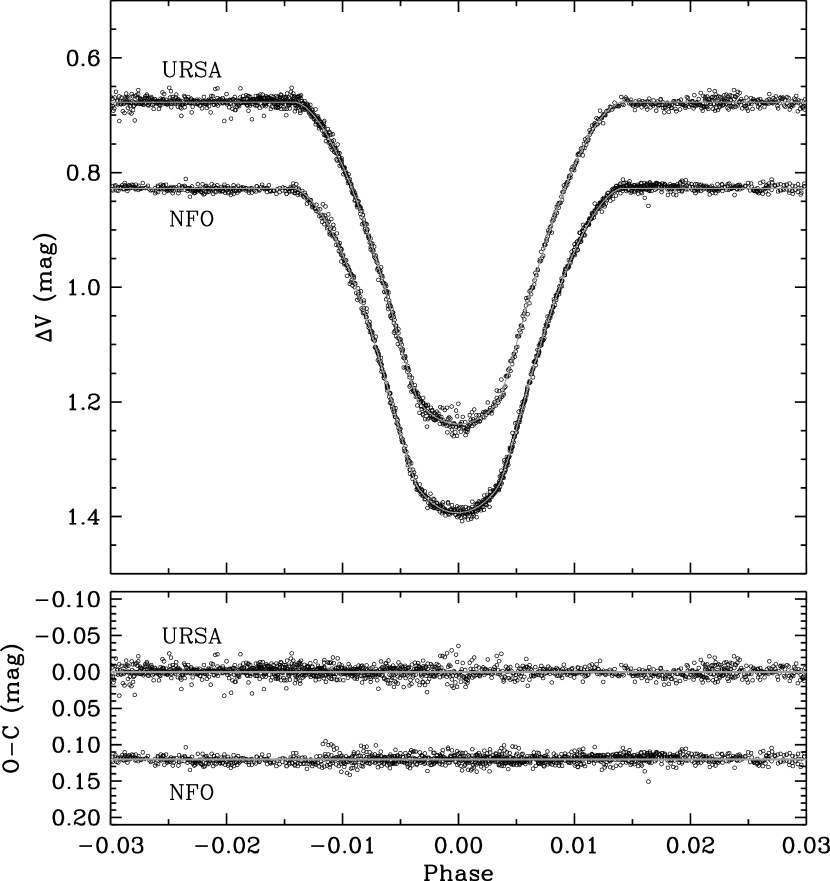
Figure 6.— URSA and NFO differential $V$-band observations of V530 Ori near primary eclipse, shown with our best model fits. Residuals from the fits are shown at the bottom, with those from NFO displaced vertically for clarity.

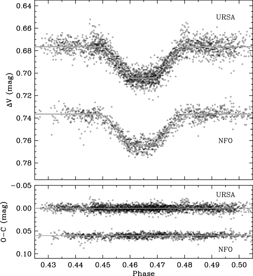
Figure 7.— URSA and NFO differential $V$-band observations of V530 Ori near secondary eclipse, shown with our best model fits. Note the different vertical scale compared to Figure 6. Residuals from the fits are shown at the bottom, with those from NFO displaced vertically for clarity. The large open circles on the ascending branch mark the time of the ROSAT X-ray observation described in Sect. 8.2.1.

Table 9Light curve solutions for V530 Ori.

Parameter	$u$	$v$	$b$	$y$	URSA $V$	NFO $V$	Adopted
$J_{\rm B}$	0.0066	0.0200	0.0537	0.0867	0.0758	0.0739	string$0.075\pm 0.002$
$r_{\rm A}+r_{\rm B}$	0.0971	0.0960	0.0964	0.0956	0.0941	0.0950	$0.0953\pm 0.0010$
$r_{\rm A}$	0.0615	0.0602	0.0604	0.0598	0.0587	0.0594	$0.0596\pm 0.0008$
$r_{\rm B}$	0.0356	0.0358	0.0360	0.0358	0.0354	0.0357	$0.0357\pm 0.0004$
$k\equiv r_{\rm B}/r_{\rm A}$	0.578	0.595	0.596	0.599	0.604	0.600	$0.600\pm 0.004$
$i$ (deg)	89.82	89.63	89.67	89.82	89.82	89.80	$89.78\pm 0.08$0
$e$	0.0779	0.0801	0.0851	0.0862	0.0863	0.0870	$0.0862\pm 0.0010$
$\omega_{\rm A}$ (deg)	130.26	130.11	130.19	129.94	130.10	130.08	$130.08\pm 0.14$00
$u_{\rm A}$	0.92	0.75	0.64	0.52	0.48	0.54	$\cdots$
$u_{\rm B}$	0.78	0.75	0.79	0.72	0.71	0.71	$\cdots$
$\ell_{\rm A}$	0.9974	0.9928	0.9822	0.9720	0.9753	0.9756	$\cdots$
$\ell_{\rm B}$	0.0024	0.0070	0.0176	0.0278	0.0245	0.0242	$\cdots$
$\ell_{\rm B}/\ell_{\rm A}$	0.002	0.007	0.018	0.029	0.025	0.025	$\cdots$
$\sigma$ (mmag)	10.960	8.700	7.821	7.165	6.678	5.131	$\cdots$
$N$	720	720	720	720	5137	3024	$\cdots$

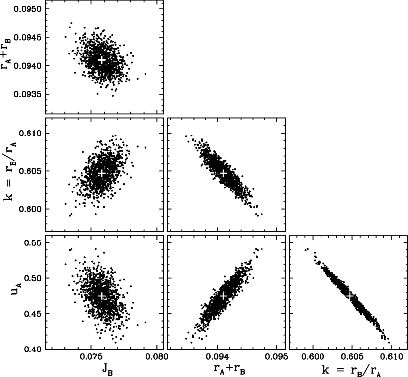
Figure 8.— Results from Monte Carlo simulations with JKTEBOP using the URSA data set, illustrating the correlations among some of the main elements: $J_{\rm B}$, $r_{\rm A}+r_{\rm B}$, $k\equiv r_{\rm B}/r_{\rm A}$, and the primary linear limb-darkening parameter $u_{\rm A}$. Plus signs represent the median values for each variable.

Our solutions consistently indicate that the secondary eclipse (only 0.028 mag deep in $V$) is total, with a duration of totality of about 70 minutes. The primary eclipse is annular. Trials were made allowing for the possible presence of third light, but the resulting values were not significantly different from zero, so no third light was allowed in the final solutions. Additional trials were carried out using a non-linear limb-darkening law of the logarithmic type (Claret, 2000), and also a quadratic law, but we found the residual variances of the fits to be always worse than with the linear limb-darkening law. The resulting fitted orbital parameters were not significantly different from those with the linear law, except that the logarithmic law preferred a primary relative radius value ($r_{\rm A}$) about 1% larger, and the quadratic law gave a value about 1.9% larger. Because the fit to the data is superior for the linear law, we have chosen those results for the remainder of this study. Average values of the geometric properties used for computing the absolute dimensions are listed in the last column of Table 9.

7. Absolute dimensions

Masses and radii for the components of V530 Ori computed from the information in Table 3 and Table 9 are presented in Table 10, and are determined to better than 0.7% in the case of the masses and 1.3% for the radii. Based on the three detailed and independent chemical analyses in Sect. 4, the average metallicity of V530 Ori (assuming the primary and secondary to have the same composition) is determined to be ${\rm[Fe/H]}=-0.12\pm 0.08$. A photometric estimate in good agreement with this value was obtained using the Strömgren indices in Sect. 5 weight-averaged with those measured by Lacy (2002), along with the calibration in Eq. 14 by Olsen (1984). The result is ${\rm[Fe/H]}=-0.10\pm 0.13$, which should be unaffected by the very faint secondary. Use of the calibration by Holmberg et al. (2007) yields a somewhat lower value of ${\rm[Fe/H]}=-0.23\pm 0.09$, still in agreement with the more reliable spectroscopic determination.

The procedure described in Sect. 3 to determine template parameters for deriving RVs can be refined by interpolating between grid points in our libraries of synthetic spectra, in order to determine more precise values for $T_{\rm eff}$ and $v\sin i$. The $v\sin i$ value for the primary obtained in this way, $9\pm 1$ km s^-1, is consistent with what is expected if the star were rotating pseudo-synchronously (see Table 10; Hut, 1981), and is in agreement with predictions from theory suggesting a synchronization timescale of only $\sim$10⁷ yr (Sect. 3), much shorter than the system age estimated below. However, the resulting temperature for that star from this method depends on the metallicity adopted, due to strong correlations between those two properties. We performed the determinations with [Fe/H] values of 0.0 and $-0.5$, and then interpolated to ${\rm[Fe/H]}=-0.12$, separately for our DS, TRES, and KPNO spectra. The $T_{\rm eff}$ values obtained for the primary are 5880 K, 5880 K, and 5820 K, respectively, which are similar to those derived from disentangling (Sect. 4). They have estimated uncertainties of 100 K. The accuracy of our various (non-independent) temperature determinations for the primary star, which we have summarized in Table 4, is likely limited by systematic effects not reflected in the formal uncertainties. For the analysis that follows we have adopted a consensus temperature for the primary of $5890\pm 100$ K, in which the uncertainty is a conservative estimate that is approximately equal to half the spread in the spectroscopic determinations. The secondary temperature was inferred from this value and the temperature difference, $\Delta T_{\rm eff}$. The latter may be derived from the central surface brightness ratio $J_{\rm B}$ (Table 9) using the absolute visual flux calibration of Popper (1980). As this procedure is entirely differential, the resulting temperature difference, $\Delta T_{\rm eff}=2010\pm 70$ K is typically better determined than the individual temperatures. The adopted $T_{\rm eff}$ value for the secondary is then $3880\pm 120$ K. These stellar temperatures correspond approximately to spectral types of G1 and M1 for the primary and secondary. We note, finally, that the small differences between these final stellar properties and the template parameters adopted in Sect. 3 for the RV determinations have a negligible effect on those measurements.

Table 10Physical properties of V530 Ori.

Parameter	Star A	Star B
Mass ($M_{\sun}$)	1.0038 $\pm$ 0.0066	0.5955 $\pm$ 0.0022
Radius ($R_{\sun}$)	0.980 $\pm$ 0.013	0.5873 $\pm$ 0.0067
$\log g$ (cgs)	4.457 $\pm$ 0.012	4.676 $\pm$ 0.010
$T_{\rm eff}$ (K)	5890 $\pm$ 1000	3880 $\pm$ 1200
$\Delta T_{\rm eff}$ (K)	$2010~{}\pm~{}70$00
$a$ ($R_{\sun}$)	16.450 $\pm$ 0.0300
$v_{\rm sync}\sin i$ (km s-1)	8.1 $\pm$ 0.1	4.9 $\pm$ 0.1
$v_{\rm psync}\sin i$ (km s-1)	8.5 $\pm$ 0.1	5.1 $\pm$ 0.1
$v\sin i$ (km s-1)	9 $\pm$ 1	$\cdots$
$\log L/L_{\sun}$	0.016 $\pm$ 0.032	$-$1.154 $\pm$ 0.053+
$L_{\rm B}/L_{\rm A}$	0.068 $\pm$ 0.009
$M_{\rm bol}$ (mag)	4.693 $\pm$ 0.079	7.62 $\pm$ 0.13
$F_{V}$	3.7586 $\pm$ 0.0098	3.468 $\pm$ 0.011
$M_{V}$ (mag)	4.71 $\pm$ 0.10	8.72 $\pm$ 0.11
$E(B-V)$ (mag)	0.045 $\pm$ 0.020
$V-M_{V}$ (mag)	5.06 $\pm$ 0.12
Distance (pc)	103 $\pm$ 600
${\rm[Fe/H]}$	$-0.12\pm 0.08$+

The reddening towards V530 Ori was estimated in several ways. One comes from the Strömgren photometry and the calibration by Crawford (1975), and gives $E(B-V)=0.059$. Five other $E(B-V)$ values were inferred from the extinction maps of Burstein & Heiles (1982), Hakkila et al. (1997), Schlegel et al. (1998), Drimmel et al. (2003), and Amôres & Lépine (2005) for an assumed distance of 100 pc. The results, 0.071, 0.039, 0.052, 0.019, and 0.030, were averaged with the previous one to yield an adopted reddening of $E(B-V)=0.045\pm 0.020$, with a conservative uncertainty. A consistency check on the effective temperature adopted above may be obtained from standard photometry available for V530 Ori from various catalogs and other literature sources (Tycho-2, Høg et al. 2000; 2MASS, Cutri et al. 2003; TASS, Droege et al. 2006; APASS, Henden et al. 2012; Lacy 1992b; Lacy 2002; and Sect. 5). From eleven appropriately de-reddened non-independent color indices and the calibrations of Casagrande et al. (2010) (for the above adopted spectroscopic metallicity) we obtained $T_{\rm eff}=5800\pm 100$ K, which corresponds to the combined light of the two stars as the secondary has a non-negligible influence on the photometry, especially at the redder wavelengths. Individual temperatures for the components may then be inferred using the absolute visual flux calibration of Popper (1980), and are $T_{\rm eff}=5920$ K for the primary and 3900 K for the secondary, with estimated uncertainties of 100 K. The primary value is consistent with our earlier spectroscopic estimates (Table 4).

The distance to V530 Ori is listed also in Table 10, along with other derived properties; it relies on an average out-of-eclipse brightness of $V=9.886\pm 0.004$ based on the literature sources cited above, corrected for extinction using $A(V)=3.1E(B-V)$. Separate distance calculations for the two components yield consistent results.

8. Comparison with theory

8.1. Standard models

Our knowledge of the metallicity of V530 Ori presents an opportunity for a stringent test of models of stellar evolution against our highly accurate mass, radius, and temperature measurements, with one less free parameter than is common in these types of comparisons. This is particularly important in this case because the system contains an M star, for which abundance analyses are usually very challenging and generally unavailable. A first test is shown in Figure 9, using the models from the Yonsei-Yale series (Yi et al., 2001; Demarque et al., 2004). These models are intended for solar-type stars, and adopt gray boundary conditions between the interior and the photosphere that are adequate for stars more massive than about 0.7 $M_{\odot}$, but become less realistic for lower-mass stars such as the secondary of V530 Ori. Consequently, we compare them only against the primary, which is very similar to the Sun. As shown in the figure, an evolutionary track for the measured mass of the star and its measured metallicity is in near perfect agreement with its temperature and surface gravity, at an age of about 3.3 Gyr. The star is approaching the half-way point of its main-sequence phase. Consistent with this old age, there is no sign of the Li I $\lambda$6708 absorption line in the disentangled spectra of either star.

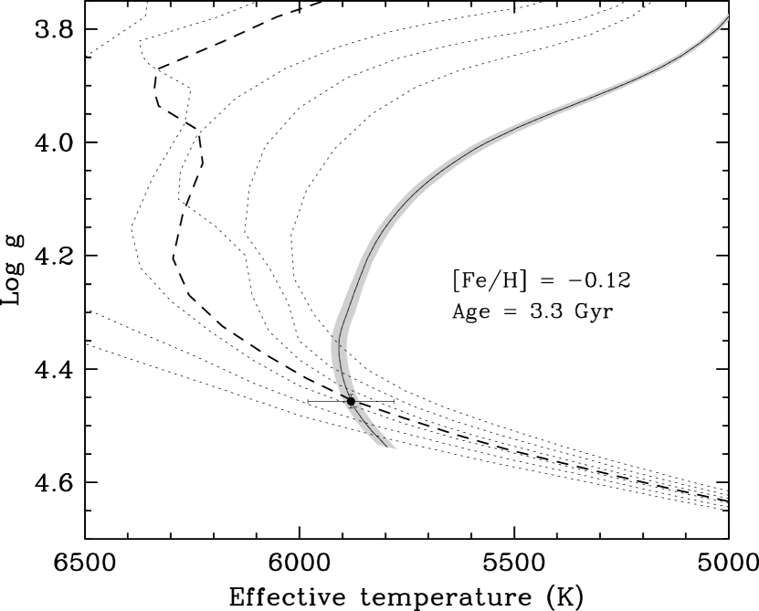
Figure 9.— Measurements for the primary of V530 Ori compared against models from the Yonsei-Yale series by Yi et al. (2001); Demarque et al. (2004) for the measured metallicity of ${\rm[Fe/H]}=-0.12$. The solid line is an evolutionary track for the measured mass, and the shaded area around it represents the uncertainty in the location of the track coming from the mass uncertainty. Isochrones from 1 to 6 Gyr are shown with dotted lines, and the one rendered with a dashed line corresponds to the best fit for an age of about 3.3 Gyr.

Figure 10 shows a comparison with model isochrones from the Dartmouth series (Dotter et al., 2008), which are appropriate both for solar-type and lower-mass stars. A 3 Gyr isochrone computed for the metallicity of the system reproduces the radius of the primary star at its measured mass, but underestimates the size of the secondary by about 2.5% (see inset in the top panel of the figure). This same isochrone is consistent with the temperature of the primary, within its uncertainty, but slightly overestimates that of the secondary. Similar anomalies in radius and temperature have been seen in many other M dwarfs, and are attributed to the effects of stellar activity and/or magnetic fields (for a recent review of this phenomenon see Torres, 2013, and references therein). One such system of M dwarfs is YY Gem (Torres & Ribas, 2002; Torres et al., 2010), whose two identical components happen to have virtually the same mass and $T_{\rm eff}$ as the secondary of V530 Ori, but a radius that is 5% larger. While age and composition differences may be part of the explanation, variances in the activity levels (YY Gem being much more active) are likely to play a significant role as well.

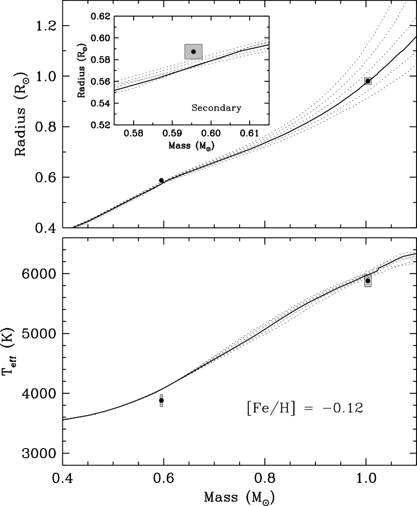
Figure 10.— Measured properties of V530 Ori compared with the Dartmouth models by Dotter et al. (2008). Top: Mass-radius diagram showing isochrones from 1 to 6 Gyr for the measured metallicity of ${\rm[Fe/H]}=-0.12$, with the solid line representing the isochrone that best fits the primary star (3 Gyr). The inset shows an enlargement around the secondary, which is seen to be larger than predicted. Bottom: Mass-temperature diagram with the same isochrones as above.

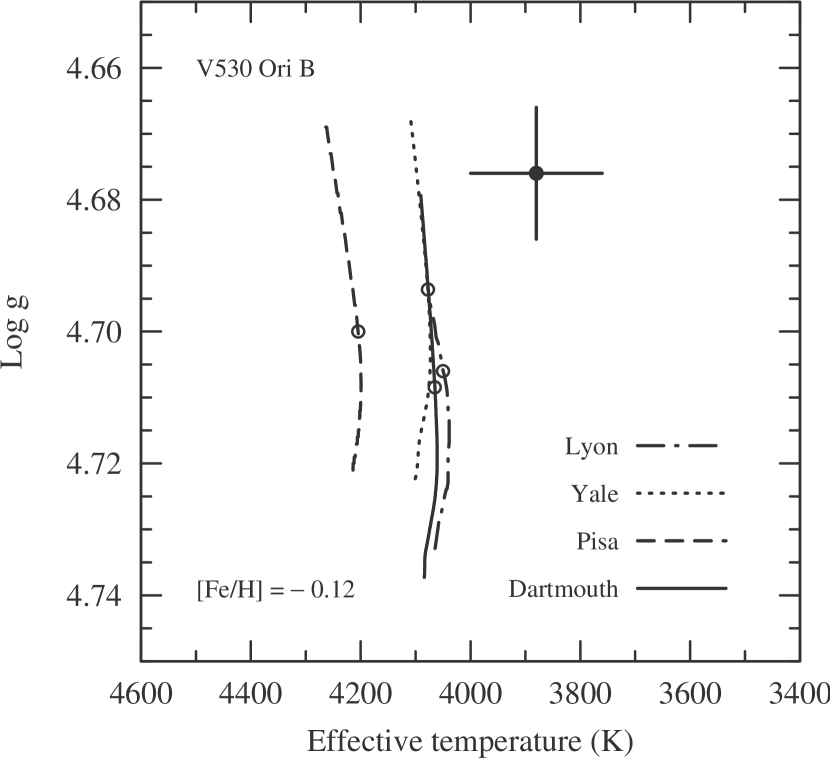
Figure 11.— Properties for the low-mass secondary of V530 Ori (solid circle with error bars) shown against evolutionary tracks for a mass of 0.6 $M_{\sun}$ similar to that measured for the star, and ages of 140 Myr to 10 Gyr. Models represented are those from Lyon (Baraffe et al., 1997, 1998), Yale (Spada et al., 2013), and Pisa (Dell’Omodarme et al., 2012), interpolated to the measured metallicity of the system or at the nearest composition available (see text). Also shown for reference is a track from the Dartmouth series. Open circles on each track mark the properties of the secondary at the age predicted by models of the primary. In all cases the models underestimate the secondary radius (i.e., they overestimate $\log g$) and predict temperatures that are too hot.

Several other series of models have been published in recent years that incorporate realistic physical ingredients appropriate for low-mass stars such as the secondary of V530 Ori (non-gray boundary conditions, improved high-density/low-temperature equations of state). These include the PARSEC models from the Padova series (Chen et al., 2014), calculations from the Yale group (Spada et al., 2013), and from the Pisa group (Dell’Omodarme et al., 2012). Older models that are also appropriate and are still widely used are those from the Lyon group (Baraffe et al., 1997, 1998). Figure 11 presents a comparison in the $\log g$ vs. $T_{\rm eff}$ diagram of the measured properties for V530 Ori B against evolutionary tracks from most of the above models for a mass of 0.6 $M_{\sun}$, conveniently very close to the measured mass of 0.5955 $M_{\sun}$. Tracks are shown for ages from 140 Myr to 10 Gyr, with open circles marking the predicted properties of the secondary at the best-fit age for the primary in each model. We include also a 0.5955 $M_{\sun}$ model from the Dartmouth series, for reference. We point out, however, that such comparisons are not always straightforward, or even possible in some cases, due to coarseness of the model grids, limitations in the set of parameters available (metallicity, mixing length parameter), and the need to interpolate among existing models, which most likely limits the accuracy. In particular, we have not compared against the Padova models as only isochrones (but not yet evolutionary tracks) are available. The Pisa track shown in Figure 11 is for the highest metallicity available ($Z=0.01$), which is marginally lower than we measure for V530 Ori. For the Lyon models interpolation to the measured metallicity of ${\rm[Fe/H]}=-0.12$ is only possible for a mixing length parameter of $\alpha_{\rm ML}=1.0$, whereas all other models adopt a solar-calibrated value of $\alpha_{\rm ML}$. Additionally, there are differences in the interior compositions adopted in all these calculations, and in many other details that may explain why the predictions differ from model to model, though a thorough discussion of these issues is beyond the scope of this paper. Nevertheless, a common pattern seen in the figure is that all models overestimate the temperature of the secondary star by 4–8%, and also overestimate its surface gravity, which means they underestimate the radius (by about 2 to 4%). These discrepancies are in the same direction as found previously for many other low-mass stars.

Additional differences between models and observations for V530 Ori are seen when comparing the secondary/primary flux ratios we estimated spectroscopically and photometrically (Sect. 3 and Sect. 6) against predictions for stars with the exact masses we measure. We illustrate this in Figure 12, in which the predictions in several standard photometric passbands are based on the same 3 Gyr Dartmouth isochrone that provided the best fit to the mass and radius of the primary in Figure 10. Models systematically underestimate all of the measured flux ratios by roughly a factor of two, with the absolute deviations increasing toward longer wavelengths. This is not entirely unexpected, given that the models also fail to match the radius and temperature of the secondary star, as well as its bolometric luminosity, which is overestimated. Interestingly, we find that arbitrarily increasing the secondary mass to $M_{\rm B}=0.64$ $M_{\sun}$ leads to predictions that agree nearly perfectly with all of the measured flux ratios (bottom panel of Figure 12), from Strömgren $u$ to the value measured from our KPNO spectra at $\sim$6410 Å, close to the $R_{\rm C}$ band. This is unlikely to be a coincidence. We note, though, that a mass for the secondary of $0.64$ $M_{\sun}$ (nearly 7% larger than measured, or $\sim$18$\sigma$) is implausibly large given our observational uncertainties, and would not make the fit to the other global properties ($R$, $T_{\rm eff}$) any better. The reason for the underpredicted $\ell_{\rm B}/\ell_{\rm A}$ values may be related to deficiencies in the temperature-color transformations adopted in the Dartmouth models, which are based on PHOENIX model atmospheres (Hauschildt et al., 1999a, b), and which are known to degrade rapidly at optical wavelengths for cooler stars. Even so, one might expect the predictive power of these models to be better when considering flux ratio differences between one wavelength and another (e.g., the difference between $[\ell_{\rm B}/\ell_{\rm A}]_{y}$ and $[\ell_{\rm B}/\ell_{\rm A}]_{\rm D51}$), because those rely on theory only in a differential sense. This is indeed what we see in Figure 12, and we take this to represent indirect support for the accuracy of our light curve solutions in Sect. 6 (performed independently in each passband), and therefore of the accuracy of the measured stellar radii.

Figure 12.— Top: Measured flux ratios ($\ell_{\rm B}/\ell_{\rm A}$) from our spectroscopic and photometric analyses of V530 Ori compared against predictions from the Dartmouth models of Dotter et al. (2008) for the measured masses of the two stars. Theoretical values for a number of standard photometric passbands are marked with open squares and connected with a line, and were computed using the same 3 Gyr, ${\rm[Fe/H]}=-0.12$ best-fit isochrone from Fig. 10. Passbands labeled include Strömgren $uvby$, Sloan $gri$, Johnson-Cousins $BV(RI)_{\rm C}$, and D51, whose central wavelength coincides with the Mg I b triplet, and therefore closely matches the spectroscopic window of our DS and TRES observations. Bottom: Same as above, changing the secondary mass to be 0.64 $M_{\sun}$ instead of the measured value of 0.5955 $M_{\sun}$.

8.2. Magnetic models

A series of stellar models were computed using the magnetic Dartmouth stellar evolution code (Feiden & Chaboyer, 2012, 2013) to test the idea that magnetic fields are responsible for the observed anomalies between the secondary in V530 Ori and stellar models. The aim of the present analysis is to first determine whether magnetic models are able to provide a consistent solution for the two components of V530 Ori, and then, if a consistent solution is identified, to establish whether the conditions presented by the models are physically plausible.

Prior to implementing magnetic fields in the stellar evolution calculations, as a check we re-assessed the performance of the standard (i.e., non-magnetic) models from the magnetic Dartmouth code owing to small differences with the original Dartmouth models of Dotter et al. (2008). Comparisons were carried out in the age-radius and age-$T_{\rm eff}$ planes for mass tracks computed at the precise masses and metallicity of the V530 Ori stars. Figure 13 shows that properties of the primary star are well reproduced by the model (represented with a solid line) between 2.7 and 3.5 Gyr, yielding an age of $3.1\pm 0.4$ Gyr, similar to our earlier finding. As discussed before, the properties of the secondary are not reproduced by the corresponding standard model. Instead, theory predicts a radius that is 3.7% too small and a temperature that is 4.8% too hot compared to observations. Given that standard models match the properties of the primary to a large degree, we began our magnetic model analysis by assuming only the secondary is affected by the presence of a magnetic field.

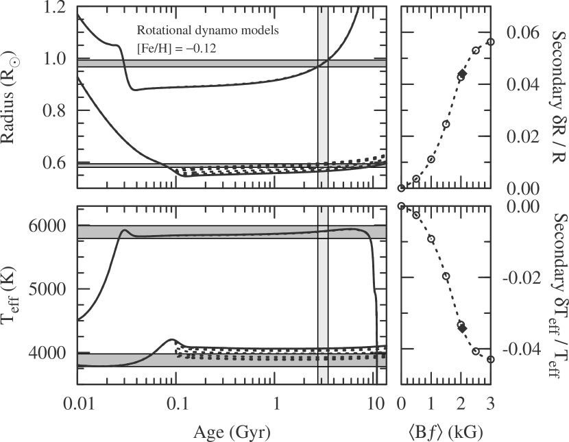
Figure 13.— Left: Dartmouth models for the metallicity of V530 Ori compared against the measured radii and temperatures of the components, represented by the horizontal bands. Standard (non-magnetic) evolutionary tracks for the precise masses of the stars are drawn with solid lines, and models incorporating magnetic fields with a rotational dynamo prescription are drawn with dotted lines. Field strengths for the secondary are $\langle Bf\rangle=$ 0.5, 1.0, 1.5, 2.0, 2.5, and 3.0 kG, and result in increasing departures from the standard models. A magnetic model with a field strength of 170 G is shown for the primary, but is nearly indistinguishable from the corresponding standard model. The best fit age range is shown by the vertical band. Right: Relative changes in radius ($\delta R/R$) and effective temperature ($\delta T_{\rm eff}/T_{\rm eff}$) for the secondary as a function of the strength of the magnetic field (see text). The best fit value is marked with a filled diamond.

A small grid of magnetic stellar models was computed at a fixed mass (0.596 $M_{\sun}$) and metallicity (${\rm[Fe/H]}=-0.12$) for V530 Ori B. Two procedures were used for modeling the influence of the magnetic field on convection that are described by Feiden & Chaboyer (2013). These two procedures were designed to roughly mimic the effects of two different dynamo actions: a rotational or shell dynamo ($\alpha$–$\Omega$) and a turbulent or distributed dynamo ($\alpha^{2}$). All models utilized a dipole radial profile as the influence of the magnetic field is only weakly dependent on the choice of radial profile for stars with a radiative core and convective envelope (Feiden & Chaboyer, 2013). For models using the rotational dynamo procedure, values of the average surface magnetic fields were $\langle Bf\rangle=$ 0.5, 1.0, 1.5, 2.0, 2.5, and 3.0 kG, while for the turbulent dynamo the values were $\langle Bf\rangle=$ 0.5, 0.6, 0.7, 0.8, 1.0, 2.0, and 3.0 kG, in which $B$ is the photospheric magnetic field strength and $f$ the filling factor. Corresponding mass tracks are show with dotted lines in Figures 13 and 14, with the relative changes in radius ($\delta R/R$) and temperature ($\delta T_{\rm eff}/T_{\rm eff}$) of the secondary indicated on the right as a function of the strength of the magnetic field.

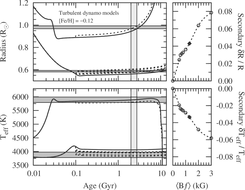
Figure 14.— Similar to Fig. 13 but for magnetic models with a turbulent dynamo. Field strengths shown for the secondary are 0.5, 0.6, 0.7, 0.8, 1.0, 2.0, and 3.0 kG (dotted lines). The magnetic model for the primary has $\langle Bf\rangle=170$ G, and produces more noticeable changes in the radius and temperature of the star than the rotational dynamo model shown in Fig. 13.

Results show that magnetic models of V530 Ori B can be made to reproduce the observed properties assuming either dynamo procedure, with the rotational dynamo suggesting $\langle Bf\rangle_{\rm B}=2.1\pm 0.4$ kG and the turbulent dynamo giving $\langle Bf\rangle_{\rm B}=1.3\pm 0.4$ kG. These values were calculated by extracting the properties of each magnetic model computed at an age of 3.1 Gyr, and generating curves using a cubic spline interpolation that give the model radius and model temperature difference between the primary and secondary as functions of $\langle Bf\rangle$ (right panels of Figures 13 and 14). The spacing of the magnetic field strength was 0.05 kG along the interpolated curves. We then computed the $\chi^{2}$ value,

$$\chi^{2}=\left(\frac{R_{\rm obs}-R_{\rm mod}}{\sigma_{R}}\right)^{2}+\left(\frac{\Delta T_{\rm eff,\,obs}-\Delta T_{\rm eff,\,mod}}{\sigma_{\Delta T}}\right)^{2},$$

at each point along the interpolated curve and took the resulting minimum as the best-fit $\langle Bf\rangle$. For completeness, we note that the minimum $\chi^{2}$ value we found is $\chi^{2}_{\rm min}=0.4$. Approximate errors for the permitted model $\langle Bf\rangle$ were determined by satisfying the condition $\chi^{2}(\langle Bf\rangle)=\chi_{\rm min}^{2}+1$.

As shown earlier, the primary star is active as well and may be similarly influenced by its magnetic field, even though standard models seem to be able to match the observed properties without that effect. To test this, we generated magnetic models for the primary star guided by an estimate of the field strength, described in the next section, of $\langle Bf\rangle_{\rm A}=170$ G. Results using the rotational dynamo formulation are shown in Figure 13, but produce only a negligible departure from the standard model mass track. Figure 14, on the other hand, demonstrates that the turbulent dynamo model causes a greater level of radius inflation and temperature suppression in the primary. Temperature suppression is such that agreement is nearly lost between the model and the observations. The age prediction is reduced to $2.4\pm 0.4$ Gyr, and magnetic models of the secondary require moderately stronger $\langle Bf\rangle$ values with the turbulent dynamo than in the previous case. Performing the same procedure as before to generate the best fit value, we obtained $\langle Bf\rangle_{\rm B}=1.7\pm 0.3$ kG. However, in this case we found $\chi^{2}_{\rm min}=3.5$, indicating the final fit is poor. This is driven by the fact that the temperature difference is more difficult to fit given the significantly lower temperature of the primary model with a magnetic field.

8.2.1 Magnetic field strengths: empirical estimates

Observational evidence for activity in V530 Ori is clear in the case of the primary, and although no direct signs of it are seen for the very faint secondary, we expect that star to be active as well. Approximate magnetic field strengths for both stars were estimated as follows. Saar (2001) has shown there is a power-law relationship between $\langle Bf\rangle$ and the Rossby number, $Ro\equiv P_{\rm rot}/\tau_{\rm c}$, where $P_{\rm rot}$ is the rotation period of the star and $\tau_{\rm c}$ the convective turnover time. The Rossby number for the primary may be estimated by noting that our spectroscopic $v\sin i$ measurement suggests it is rotating either synchronously or pseudo-synchronously. We will assume the latter here, although the difference is very small (see Table 10). This leads to a rotation period of $P_{\rm rot}\approx 5.84$ days based on the measured orbital eccentricity (see Hut, 1981). For $\tau_{\rm c}$ we must rely on theory. Since the calibration of Saar (2001) used convective turnover times taken from the work of Gilliland (1986), we have done the same here for consistency, and adopted (based on the temperature of 5890 K) $\tau_{\rm c}=13.8\pm 2$ days, with a conservative uncertainty. The resulting Rossby number for V530 Ori A is $Ro=0.423\pm 0.067$. A similar calculation for the secondary gives $Ro=0.116\pm 0.005$ based on $\tau_{\rm c}=50.3\pm 2$ days (Gilliland, 1986), from its temperature of 3880 K, and assuming pseudo-synchronous rotation (justified in view of the very short timescale for synchronization compared to the age of the system; see Sect. 3). The Saar (2001) relation then projects a magnetic field strength for the primary of $\langle Bf\rangle_{\rm A}=170\pm 140$ G, and a value for the secondary of $\langle Bf\rangle_{\rm B}=830\pm 650$ G, where the uncertainties account for all observational errors as well as the scatter of the calibration. The field strength for the secondary is not far from the values required by the models in the previous section, suggesting the theoretical predictions are at least plausible.

A consistency check on the empirically estimated $\langle Bf\rangle$ values may be obtained by relating these field strengths to X-ray luminosities, and comparing them against a measure of the total X-ray emission from V530 Ori detected by the ROSAT satellite. Indeed, Pevtsov et al. (2003) showed in a study of magnetic field observations of the Sun and active stars that there is a fairly tight power-law relationship between the X-ray luminosity and the total unsigned surface magnetic flux, $\Phi=4\pi R^{2}\langle Bf\rangle$, which is valid over many orders of magnitude. An updated relation restricted to dwarf stars was presented by Feiden & Chaboyer (2013). Using this latter relation along with the measured stellar radii we obtain $\log L_{\rm X,A}=28.63\pm 0.59$ and $\log L_{\rm X,B}=29.14\pm 0.57$ (with $L_{\rm X}$ in erg s^-1). The sum of the X-ray luminosities corresponds to $\log L_{\rm X,A+B}=29.26\pm 0.46$. The entry for V530 Ori in the ROSAT All-Sky Survey Faint Source Catalog (Voges et al., 2000) lists a count rate of $0.0151\pm 0.0072$ cts s^-1 (0.1–2.4 keV) and a hardness ratio of ${\rm HR1}=-0.43\pm 0.37$ for the system, from a 465 s exposure. The corresponding total X-ray luminosity computed using the energy conversion factor given by Fleming et al. (1995) and the distance in Table 10 is $\log L_{\rm X}{\rm(ROSAT)}=29.06\pm 0.33$. The good agreement between this measurement and the sum of the individual X-ray luminosities, $\log L_{\rm X,A+B}$, may be taken as an indication of the accuracy of the $\langle Bf\rangle$ values reported above, even though their formal errors are large.

9. Discussion

To the extent that our empirical magnetic field estimates above represent the actual surface field strengths of the stars in V530 Ori, it seems natural to require the models for both components to account for these effects. However, the way in which the influence of magnetic fields on the stellar properties is treated in the models seems to make a significant difference, particularly for the primary star, and it is not at all clear which formulation is more realistic. Given that this issue is at the heart of the long-standing problem of radius inflation and temperature suppression in cool stars, a careful consideration of the physical assumptions is in order.

Based strictly on the agreement with our empirical estimates, a scenario whereby the primary star’s magnetic field is generated by a “rotational” dynamo and the secondary by a more “turbulent” dynamo would seem to be preferred. In this case, the magnetic field of the primary draws its energy largely from kinetic energy of (differential) rotation, with the magnetic field rooted in a strong shear layer below the convection zone (i.e., the tachocline), analogous to the mechanism believed to drive the solar dynamo (Parker, 1993; Charbonneau & MacGregor, 1997). Convection is then inhibited by the stabilizing effect that a (vertical) magnetic field has on a fluid (Gough & Tayler, 1966; Lydon & Sofia, 1995). Given the similarity of V530 Ori A to the Sun, the adoption of this magneto-convection formulation seems justified. With a surface magnetic field strength $\langle Bf\rangle_{\rm A}=170$ G, the influence of a magnetic field on the flow of convection is minimal and the structure of the model is unaffected (see Figure 13), so that the magnetic model produces results consistent with the non-magnetic model.

Concerning the secondary, both magnetic field formulations yield agreement with the stellar properties ($T_{\rm eff}$ and $R$) at an age defined by the properties of the primary (assuming the discussion above holds). At face value the turbulent dynamo approach requires a field strength ($\langle Bf\rangle=1.3\pm 0.4$ kG) that is closer to the empirically estimated value of $\langle Bf\rangle_{\rm B}=0.83\pm 0.65$ kG than the alternate approach with a rotational dynamo (which predicts $\langle Bf\rangle=2.1\pm 0.4$ kG). The accuracy of the empirical value is difficult to assess and depends strongly on the reliability of the Saar (2001) calibration. The turbulent dynamo formulation simplistically assumes that the energy for the magnetic field is provided by kinetic energy available in the larger scale convective flow. Convection is then made less efficient as energy is diverted away from convecting fluid elements thereby impeding their velocity and thus reducing the total amount of convective energy flux (e.g., Durney et al., 1993; Chabrier & Küker, 2006; Browning, 2008). Precisely how this conversion is achieved (e.g., through turbulence, helical convection, or feedback generated by the Lorentz force) is not explicitly defined in the stellar models.

While consistency between the estimated surface magnetic field strength and that required by the models is encouraging, it is not clear that the dynamo mechanism at work in V530 Ori B should be any different from that in V530 Ori A. Both stars possess a radiative core and a convective outer envelope and thus, presumably, a stable tachocline in which to produce a magnetic field through an interface dynamo. Furthermore, the presence of a stable tachocline is not necessarily a strict condition for a solar-like dynamo (Brown et al., 2010). Therefore, there is no reason a priori to believe that the stars should have a different dynamo mechanism. If we instead assume that the primary also has a dynamo driven by convection, then the structural changes imparted by the magnetic field become significant, even for a modest 170 G magnetic field at the surface. Changes induced on the primary are such that models of the primary and secondary cannot be made to agree at the same age, leaving us with precisely the same problem that we were looking to correct with the magnetic models.

A possible reason to expect a different dynamo mechanism would be if differential rotation were somehow suppressed in the secondary star. Quenching of differential rotation has been observed in detailed magneto-hydrodynamic simulations as a result of Maxwell stresses produced by an induced magnetic field (Browning, 2008). On the other hand, simulations of a Sun-like star with an angular velocity similar to V530 Ori A do not demonstrate this quenching (Brown et al., 2010), so we may posit that the primary star has a dynamo driven by differential rotation, as we initially supposed. Although the two components of V530 Ori are likely rotating with a similar angular velocity, convective velocities in the secondary are slower, leading to convective flows that are more susceptible to the influence of the Coriolis force. This could then drive strong magnetic fields that also quench the differential rotation. Unfortunately, assessing the level of differential rotation on the secondary is not currently possible.

Browning (2008) predicts that when differential rotation is quenched, the large scale axisymmetric component of the magnetic field should account for a larger fraction of total magnetic energy. Using the empirical scaling relations of Vidotto et al. (2014), we estimated the large scale magnetic field component on each star using our derived X-ray luminosities. We find that the large scale component of the magnetic field (taken to be perpendicular to the line of sight) makes up 6% and 12% of the total magnetic energy, corresponding to $\langle Bf\rangle_{\perp}=10$ G and 100 G for V530 Ori A and B, respectively. While the trend is consistent with the secondary having a more significant large scale field component (in terms of total magnetic energy contribution), it is not possible to say whether this is the result of different dynamo actions.

In summary, while many critical aspects of the problem are still not understood, the arguments above seem to support a picture in which the models are able to match the measured temperatures and radii of the components with the magnetic field playing little role in changing the structure of the primary star (i.e., consistent with it having a rotational dynamo). The nature of the magnetic field on the secondary is less clear, with the observations perhaps favoring a distributed (turbulent) dynamo over a rotational one, but not at a very significant level.

Other consequences of magnetic fields on structure of the stars in V530 Ori appear small: the predicted apsidal motion constant corresponds to an apsidal motion period of $U=19,\!400$ yr for a magnetic secondary (both dynamo types), not very different from the value of $19,\!100$ yr computed with no magnetic fields. The observed value from Sect. 2 is unfortunately much too imprecise for a meaningful comparison. We note that the properties of the system are such that the contribution to the apsidal motion from General Relativity effects (e.g., Giménez, 1985) is expected to dominate (72%) over the classical terms from tidal and rotational distortion.

A larger effect of magnetic fields is seen on the convective turnover time. The Dartmouth models yield $\tau_{c}=16$ days for the primary star, somewhat longer than other estimates mentioned earlier, and values for the secondary of 50.5 days (standard, non-magnetic), 49.3 days (rotational dynamo), and 65.4 days (turbulent dynamo).

10. Concluding remarks

With masses and radii determined to better than 0.7% and 1.3%, respectively, and a secondary of spectral type M1, V530 Ori joins the ranks of the small group of eclipsing binary systems containing at least one low-mass main-sequence star with well-measured properties. What distinguishes this example is that the chemical composition is well known from our detailed analysis of the disentangled spectrum of the primary component, which is an easily studied G1 star. Investigations of most other systems containing M stars have struggled to infer metallicities directly from the molecule-ridden spectra of the M stars, or by more indirect means. Knowledge of the metallicity removes a free parameter in the comparison with stellar evolution models that permits a more meaningful test of theory, as we have done here. We have also made a special effort to establish an accurate temperature for the primary star by measuring it in several different ways, as the $T_{\rm eff}$ value for the secondary hinges on it, as does the entire comparison with models.

Both the Yonsei-Yale and the Dartmouth models provide a good match to the primary star at the measured metallicity, suggesting that both its temperature and metallicity are accurate. On the other hand, we find that standard models from the Dartmouth series underpredict the radius and overpredict the temperature of the secondary by several percent, as has been found previously for many other cool main-sequence stars. Magnetic models from the same series succeed in matching the observed radii and temperatures of both stars at their measured masses with surface magnetic fields for the secondary of about 1–2 kG in strength, fairly typical of early M dwarfs, and an age of some 3 Gyr. These field strengths are not far from what we estimate empirically for V530 Ori B on the basis of the Rossby numbers. The agreement is reassuring, and suggests that we are closer to understanding radius inflation and temperature suppression for convective stars, not only qualitatively but also quantitatively. Earlier quantitative evidence in this direction was presented by Feiden & Chaboyer (2012, 2013, 2014), also for the Dartmouth models, with the present case being perhaps a stronger test in that our estimates of the individual magnetic field strengths used somewhat weaker assumptions. V530 Ori is thus a key benchmark system for this sort of test. Questions remain, however, about the exact nature of the magnetic fields and how their effect on the global properties of the stars should be treated in the models (rotational dynamo, turbulent dynamo, or some other prescription).

References

- Amôres & Lépine (2005) Amôres, E. B., & Lépine, J. R. D. 2005, AJ, 130, 659
- Asplund et al. (2009) Asplund, M., Grevesse, N., Sauval, A. J., & Scott, P. 2009, ARA&A, 47, 481
- Bagnuolo & Gies (1991) Bagnuolo, W. G., Jr., & Gies, D. R. 1991, ApJ, 376, 266
- Baraffe et al. (1997) Baraffe, I., Chabrier, G., Allard, F., & Hauschildt, P. H. 1997, A&A, 327, 1054
- Baraffe et al. (1998) Baraffe, I., Chabrier, G., Allard, F., & Hauschildt, P. H. 1998, A&A, 337, 403
- Bensby et al. (2014) Bensby, T., Feltzing, S, & Oey M. S. 2014, A&A, 562, A71
- Brown et al. (2010) Brown, B. P., Browning, M. K., Brun, A. S., Miesch, M. S., & Toomre, J. 2010, ApJ, 711, 424
- Browning (2008) Browning, M. K. 2008, ApJ, 676, 1262
- Burstein & Heiles (1982) Burstein, D., & Heiles, C. 1982, AJ, 87, 1165
- Casagrande et al. (2010) Casagrande, L., Ramírez, I., Meléndez, J., Bessell, M., & Asplund, M. 2010, A&A, 512, 54
- Chabrier et al. (2007) Chabrier, G., Gallardo, J., & Baraffe, I. 2007, A&A, 472, L17
- Chabrier & Küker (2006) Chabrier, G., & Küker, M. 2006, A&A, 446, 1027
- Charbonneau & MacGregor (1997) Charbonneau, P., & MacGregor, K. B. 1997, ApJ, 486, 502
- Chen et al. (2014) Chen, Y., Girardi, L., Bressan, A., et al. 2014, MNRAS, in press (arXiv:1409.0322)
- Claret (1998) Claret, A. 1998, A&AS, 131, 395
- Claret (2000) Claret, A. 2000, A&A, 363, 1081
- Claret & Hauschildt (2003) Claret, A., & Hauschildt, P. H. 2003, A&A, 412, 241
- Clausen et al. (2008) Clausen, J. V., Vaz, L. P. R., García, J. M., Giménez, A., Helt, B. E., Olsen, E. H., & Andersen, J. 2008, A&A, 487, 1081
- Crawford (1975) Crawford, D. L. 1975, AJ, 80, 955
- Cutri et al. (2003) Cutri, R. M. et al. 2003, The 2MASS All-Sky Catalog of Point Sources, Univ. of Massachusetts and Infrared Processing and Analysis Center (IPAC/California Institute of Technology)
- Dell’Omodarme et al. (2012) Dell’Omodarme, M., Valle, G., Degl’Innocenti, S., & Prada Moroni, P. G. 2012, A&A, 540, A26
- Demarque et al. (2004) Demarque, P., Woo, J.-H., Kim, Y.-C., & Yi, S. K. 2004, ApJS, 155, 667
- Díaz-Cordovés et al. (1995) Díaz-Cordovés, J., Claret, A., & Giménez, A. 1995, A&AS, 110, 329
- Diethelm (2009) Diethelm, R. 2009, IBVS, 5894
- Diethelm (2011) Diethelm, R. 2011, IBVS, 5992
- Dotter et al. (2008) Dotter, A., Chaboyer, B., Jevremović, D., et al. 2008, ApJS, 178, 89
- Drimmel et al. (2003) Drimmel, R., Cabrera-Lavers, A., & López-Corredoira, M. 2003, A&A, 409, 205
- Droege et al. (2006) Droege, T. F., Richmond, M. W., & Sallman, M. 2006, PASP, 118, 1666
- Durney et al. (1993) Durney, B. R., De Young, D. S., & Roxburgh, I. W. 1993, Sol. Phys., 145, 207
- Feiden & Chaboyer (2012) Feiden, G. A., & Chaboyer, B. 2012, ApJ, 761, 30
- Feiden & Chaboyer (2013) Feiden, G. A., & Chaboyer, B. 2013, ApJ, 779, 183
- Feiden & Chaboyer (2014) Feiden, G. A., & Chaboyer, B. 2014, ApJ, 789, 53
- Fleming et al. (1995) Fleming, T. A., Molendi, S., Maccacaro, T., & Wolter, A. 1995, ApJS, 99, 701
- Fűrész (2008) Fűrész, G. 2008, PhD thesis, Univ. Szeged, Hungary
- Gilliland (1986) Gilliland, R. L. 1986, ApJ, 300, 339
- Giménez (1985) Giménez, A. 1985, ApJ, 297, 405
- Gough & Tayler (1966) Gough, D. O., & Tayler, R. J. 1966, MNRAS, 133, 85
- Grauer et al. (2008) Grauer, A. D., Neely, A. W., & Lacy, C. H. S. 2008, PASP, 120, 992
- Hadrava (1995) Hadrava, P. 1995, A&AS, 114, 393
- Hakkila et al. (1997) Hakkila, J., Myers, J. M., Stidham, B. J., & Hardmann, D. H. 1997, AJ, 114, 2043
- Hauschildt et al. (1999b) Hauschildt, P. H., Allard, F., Ferguson, J., Baron, E., & Alexander, D. R. 1999b, ApJ, 525, 871
- Hauschildt et al. (1999a) Hauschildt, P. H., Allard, F., & Baron, E. 1999a, ApJ, 512, 377
- Henden et al. (2012) Henden, A. A., Levine, S. E., Terrell, D., Smith, T. C., & Welch, D. 2012, J. American Association of Variable Star Observers, 40, 430
- Hilditch (2001) Hilditch, R. W. 2001, An Introduction to Close Binary Stars (Cambridge, UK: Cambridge University Press) p. 152
- Høg et al. (2000) Høg, E., Fabricius, C., Makarov, V. V., Urban, S., Corbin, T., Wycoff, G., Bastian, U., Schwekendiek, P., & Wicenec, A. 2000, A&A, 355, L27
- Holmberg et al. (2007) Holmberg, J., Nordström, B., & Andersen, J. 2007, A&A, 475, 519
- Holmgren et al. (1999) Holmgren, D. E., Hadrava, P., Harmanec, P. et al. 1999, A&A, 345, 855
- Husser et al. (2013) Husser, T.-O., Wende-von Berg, S., Dreizler, S., et al. 2013, A&A, 553, A6
- Hut (1981) Hut, P. 1981, A&A, 99, 126
- Ilijić et al. (2004) Ilijić, S., Hensberge, H., Pavlovski, K., & Freyhammer, L. S. 2004, Spectroscopically and Spatially Resolving the Components of the Close Binary Stars, eds. R. W. Hilditch, H. Hensberge and K. Pavlovski (San Francisco:ASP), ASP Conf. Ser., 318, 111
- Isles (1988) Isles, J. 1988, Brit. Astr. Soc. Circ., 67, 11
- Kurucz (1979) Kurucz, R. L. 1979, ApJS, 40, 1
- Lacy (1990) Lacy, C. H. 1990, IBVS, 3448, 1
- Lacy (1992a) Lacy, C. H. S. 1992a, AJ, 104, 2213
- Lacy (1992b) Lacy, C. H. 1992b, AJ, 104, 801
- Lacy (2002) Lacy, C. H. 2002, AJ, 124, 1162
- Lacy (2004) Lacy, C. H. S. 2004, IBVS, 5577
- Lacy (2007) Lacy, C. H. S. 2007, IBVS, 5764
- Lacy (2011) Lacy, C. H. S. 2011, IBVS, 5972
- Lacy & Fox (1994) Lacy, C. H. S., & Fox, G. W. 1994, IBVS, 4009
- Lacy et al. (1999) Lacy, C. H. S., Markrum, K., & Ibanoglu, C. 1999, IBVS, 4737
- Lacy et al. (2010) Lacy, C. H. S., Torres, G., Claret, A., Charbonneau, D., & O’Donovan, F. T. 2010, AJ, 139, 2347
- Latham (1992) Latham, D. W. 1992, in IAU Coll. 135, Complementary Approaches to Double and Multiple Star Research, ASP Conf. Ser. 32, eds. H. A. McAlister & W. I. Hartkopf (San Francisco: ASP), 110
- Latham et al. (1996) Latham, D. W., Nordström, B., Andersen, J., Torres, G., Stefanik, R. P., Thaller, M., & Bester, M. 1996, A&A, 314, 864
- Latham et al. (2002) Latham, D. W., Stefanik, R. P., Torres, G., Davis, R. J., Mazeh, T., Carney, B. W., Laird, J. B., & Morse, J. A. 2002, AJ, 124, 1144
- Lehman et al. (2013) Lehmann, H., Southworth, J., Tkachenko, A., & Pavlovski K. 2013, A&A, 557, A79
- López Morales & Ribas (2005) López-Morales, M., Ribas, I, 2005, ApJ, 631, 1120
- Lydon & Sofia (1995) Lydon, T. J., & Sofia, S. 1995, ApJS, 101, 357
- Mayer et al. (2013) Mayer, P., Harmanec, P., & Pavlovski, K. 2013, A&A, 550, A2
- Mullan & MacDonald (2001) Mullan, D. J., MacDonald, J. 2001, ApJ, 559, 353
- Murdoch et al. (1993) Murdoch, K. A., Hearnshaw, J. B., & Clark, M. 1993, ApJ, 413, 349
- Nagai (2008) Nagai, K. 2008, Var. Star Bull. (Japan), No. 46
- Nelson & Davis (1972) Nelson, B., & Davis, W. D. 1972, ApJ, 174, 617
- Nidever et al. (2002) Nidever, D. L., Marcy, G. W., Butler, R. P., Fischer, D. A., & Vogt, S. S. 2002, ApJS, 141, 503
- Nordström et al. (1994) Nordström, B., Latham, D. W., Morse, J. A., Milone, A. A. E., Kurucz, R. L., Andersen, J., & Stefanik, R. P. 1994, A&A, 287, 338
- Olsen (1984) Olsen, E. H. 1984, A&AS, 57, 443
- Parker (1993) Parker, E. N. 1993, ApJ, 408, 707
- Pavlovski et al. (2009) Pavlovski, K., Tamajo, E., Koubský, P., Southworth, J., Yang, S., & Kolbas, V. 2009, MNRAS, 400, 791
- Pavlovski & Hensberge (2005) Pavlovski, K., & Hensberge, H. 2005, A&A, 439, 309
- Pavlovski & Hensberge (2010) Pavlovski, K., & Hensberge, H. 2010, Binaries – Key to Comprehension of the Universe, ASP Conf. Ser., 435, 207
- Pavlovski et al. (2010) Pavlovski, K., Kolbas, V., & Southworth, J. 2010, Binaries – Key to Comprehension of the Universe, ASP Conf. Ser., 435, 247
- Pavlovski & Southworth (2012) Pavlovski, K., & Southworth, J. 2012, IAU Symposium, 282, 359
- Pevtsov et al. (2003) Pevtsov, A. A., Fisher, G. H., Acton, L. W. et al. 2003, ApJ, 598, 1387
- Popper (1980) Popper, D. M. 1980, ARA&A, 18, 115
- Popper (1996) Popper, D. M. 1980, ApJS, 106, 133
- Popper & Etzel (1981) Popper, D. M., & Etzel, P. B. 1981, AJ, 86, 102
- Press et al. (1992) Press, W. H., Teukolsky, S. A., Vetterling, W. T., & Flannery, B. P. 1992, Numerical Recipes, (2nd. Ed.; Cambridge: Cambridge Univ. Press), p. 650
- Ribas (2003) Ribas, I. 2003, A&A, 398, 239
- Saar (2001) Saar, S. H. 2001, 11th Cambridge Workshop on Cool Stars, Stellar Systems and the Sun, eds. R. J. García López, R. Rebolo and M. R. Zapatero Osorio (San Francisco: ASP), ASP Conv. Ser., 223, 292
- Sahade & Berón Dávila (1963) Sahade, J., & Berón Dávila, F. 1963, Ann. Astrophys., 26, 153
- Sandberg Lacy et al. (2012) Sandberg Lacy, C. H., Torres, G., & Claret, A. 2012, AJ, 144, 167
- Schlegel et al. (1998) Schlegel, D. J., Finkbeiner, D. P., & Davis, M. 1998, ApJ, 500, 525
- Simon & Sturm (1994) Simon, K. P., & Sturm E. 1994, A&A, 281, 286
- Smalley et al. (2011) Smalley, B., Smith, K. C., & Dworetsky, M. M. 2001, uclsyn User Guide, available at http://www.astro.keele.ac.uk/ bs/publs/uclsyn.pdf
- Southworth et al. (2004) Southworth, J., Maxted, P. F. L., & Smalley, B. 2004, MNRAS, 349, 547
- Spada et al. (2013) Spada, F., Demarque, P., Kim, Y.-C., & Sills, A. 2013, ApJ, 776, 87
- Strohmeier (1959) Strohmeier, W. 1959, Veröff. der Remeis-Sternwarte, Bamberg, Band 5, Nr. 3
- Tamajo et al. (2011) Tamajo, E., Pavlovski, K., & Southworth, J. 2011, A&A, 526, A76
- Tkachenko et al. (2014) Tkachenko, A., Degroote, P., Aerts, C. et al. 2014, MNRAS, 438, 3093
- Torres (2013) Torres, G. 2013, AN, 334, 4
- Torres et al. (2010) Torres, G., Andersen, J., & Giménez, A. 2010, A&A Rev., 18, 67
- Torres, Latham & Stefanik (2007) Torres, G., Latham, D. W., & Stefanik, R. P. 2007, ApJ, 662, 602
- Torres & Ribas (2002) Torres, G., Ribas, I. 2002, ApJ, 567, 1140
- Torres et al. (1997) Torres, G., Stefanik, R. P., Andersen, J., Nordström, B., Latham, D. W., & Clausen, J. V. 1997, AJ, 114, 2764
- Torres et al. (2002) Torres, G., Neuhäuser, R., & Guenther, E. W. 2002, AJ, 123, 170 1
- Van Hamme (1993) Van Hamme, W. 1993, AJ, 106, 2096
- Vidotto et al. (2014) Vidotto, A. A., Gregory, S. G., Jardine, M., et al. 2014, MNRAS, 441, 2361
- Voges et al. (2000) Voges, W., Aschenbach, B., Boller, T. et al. 2000, IAU Circ., 7432, 3
- Yi et al. (2001) Yi, S., Demarque, P., Kin, Y.-C., Lee, Y.-W., Ree, C. H., Lejeune, T., & Barnes, S. 2001, ApJS, 136, 417
- Zucker & Mazeh (1994) Zucker, S., & Mazeh, T. 1994, ApJ, 420, 806