What is the probability that direct detection experiments have observed Dark Matter?

Abstract

In Dark Matter direct detection we are facing the situation of some experiments reporting positive signals which are in conflict with limits from other experiments. Such conclusions are subject to large uncertainties introduced by the poorly known local Dark Matter distribution. We present a method to calculate an upper bound on the joint probability of obtaining the outcome of two potentially conflicting experiments under the assumption that the Dark Matter hypothesis is correct, but completely independent of assumptions about the Dark Matter distribution. In this way we can quantify the compatibility of two experiments in an astrophysics independent way. We illustrate our method by testing the compatibility of the hints reported by DAMA and CDMS-Si with the limits from the LUX and SuperCDMS experiments. The method does not require Monte Carlo simulations but is mostly based on using Poisson statistics. In order to deal with signals of few events we introduce the so-called “signal length” to take into account energy information. The signal length method provides a simple way to calculate the probability to obtain a given experimental outcome under a specified Dark Matter and background hypothesis.

1 Introduction

Dark Matter (DM) direct detection experiments search for a tiny nuclear recoil signal induced by the scattering of a DM particle from the galactic halo with a nucleus in the detector [1]. In recent years a number of experiments have reported signals which may be interpreted in terms of DM [2, 3, 4, 5, 6, 7, 8, 9], an interpretation which however, typically is in disagreement with bounds from other experiments [10, 11, 12, 13, 14, 15, 16]. Such a conclusion depends on the assumed particle physics model for the DM–nucleus interaction as well as on assumptions for the local DM density and velocity distribution.

In this paper we are going to address the second issue by adopting methods for comparing different experiments which are independent of the assumed DM distribution. Our work is based on the so-called minimal velocity ($v_{m}$) method proposed in Refs. [17, 18], which has been applied by a number of authors, see e.g., [19, 20, 21, 22, 23, 24, 25, 26, 27, 28, 29, 30]. Usually this method is used to derive bounds on the halo integral in $v_{m}$ space from data setting limits, which then can be compared to the positive results from experiments reporting a signal. This allows a qualitative assessment whether a certain signal is in agreement or disagreement with bounds, whereas a quantitative statement on the consistency is lacking. The aim of this work is to present a way to quantify the compatibility of a positive signal with limits from other experiments, extending methods used in Ref. [22]. We are going to calculate an upper bound on the probability for both experimental outcomes (the one reporting a signal and the one setting an upper limit) to occur simultaneously, assuming the DM hypothesis.

Below we are going to consider data from the CDMS-II experiment using a silicon target [9] as well as the signal for annual modulation from DAMA [3]. We calculate the joint probability to obtain those indications in favour of DM scattering together with the results from the LUX [15] and SuperCDMS [16] experiments, which place strong limits using xenon and germanium targets, respectively. In section 2 we briefly describe the data and our analysis thereof. After setting up the notation in section 3, we review the $v_{m}$ method to set upper bounds on the halo integral in section 4. In section 5 we present our method to calculate the joint probability for observing a DM signal together with the data leading to strong limits on the scattering cross section. We consider the situation encountered in CDMS silicon data, of an excess of few events above the expected background in section 5.1, where we also introduce the “signal length” method. It provides a simple way to calculate the probability of the experimental outcome taking into account energy information of the obtained events. In section 5.2 we apply our method also to the case of DAMA observing a signal for annual modulation, both using a “trivial bound” on the modulation amplitude as well as a bound based on the expansion of the halo integral in the Earth’s velocity [31, 22]. In section 6 we show the results of our method for the case of isospin violating DM-nucleus interactions. A general discussion and conclusions follow in section 7.

In the appendix we give some details on the signal length method, which allows us to calculate the probability of obtaining a given experimental outcome taking into account the total number of events as well as their energy distribution. It is inspired by the maximum-gap method to set an upper limit [32]; for a recent review of statistical methods in astroparticle physics see Ref. [33]. In App. A.1 we derive the equation for the relevant probability needed in section 5.1. In App. A.2 we discuss some properties of the signal length test and apply it to CDMS silicon data, showing that it leads to results consistent with the standard likelihood analysis. A general discussion of the signal length test follows in App. A.3.

During the preparation of this paper, the preprint [34] by Feldstein and Kahlhoefer appeared, addressing a similar question. The method of Ref. [34] uses a test statistic based on the joint likelihood, whose distribution has to be calculated by Monte Carlo simulation. Our approach is complementary to theirs and does not require simulations. The distributions of the relevant statistics are derived analytically from Poisson or Normal distributions.

2 Description of the data used in this analysis

In order to illustrate our method with specific examples, we will use in the following the positive signals from DAMA/LIBRA [3] (DAMA for short) and the CDMS-II silicon data [9] (CDMS-Si for short) and compare them to the limits from the LUX [15] and SuperCDMS [16] experiments. Based on this selection of data sets we will demonstrate how to apply our method in the case of a positive signal consisting of few events (CDMS-Si) as well as annual modulation (DAMA). We proceed by giving a brief description of the used data and our analysis thereof.

The LUX (Large Underground Xenon) experiment has released its first results [15]. In their analysis of 85.3 live-days of data taken in the period of April to August 2013, the data is consistent with the background-only hypothesis. We consider as signal region the region below the mean of the Gaussian fit to the nuclear recoil calibration events (red solid curve in Fig. 4 of [15]) and assume an acceptance of 0.5. It can be seen from Fig. 4 of [15] that one event at 3.1 photoelectrons falls on the red solid curve. In this analysis we assume zero events make the cut. Assuming the Standard Halo Model with the Maxwellian velocity distribution and parameters chosen as in [15], we find that our 90% CL contour agrees with good accuracy with the limit set by the LUX collaboration. To find the relation between S1 and nuclear recoil energy $E_{R}$, we use Fig. 4 of [15] and find the value of S1 at the intersection of the mean nuclear recoil curve and each recoil energy contour. For the efficiency as a function of recoil energy, we interpolate the black points in Fig. 9 of [15] for events with a corrected S1 between 2 and 30 photoelectrons and a S2 signal larger than 200 photoelectrons. We multiply the efficiency from Fig. 9 of [15] by 0.5 to find the total efficiency, and set it equal to zero below $E_{R}=3$ keV.

The SuperCDMS collaboration has observed eleven events in the recoil energy range of [1.6, 10] keV with an exposure of 577 kg day of data taken with their Ge detectors between October 2012 and June 2013 [16]. The collaboration sets an upper limit on the spin-independent WIMP-nucleon cross section of $1.2\times 10^{-42}$ cm² at a WIMP mass of 8 GeV. For the detection efficiency as a function of recoil energy, we use the red curve in Fig. 1 of [16], and assume an energy resolution of 0.2 keV.

The DAMA experiment has observed a 9.3 $\sigma$ annual modulation signal during 14 annual cycles. We use the data on the modulation amplitude for the total cumulative exposure of 1.33 ton yr of DAMA/LIBRA-phase1 and DAMA/NaI given in Fig. 8 of Ref. [3]. We consider small DM masses ($\leq 20$ GeV) in this analysis, and can thus assume that the DAMA signal is entirely due to scattering on Na. For the quenching factor of Na we take $q_{\rm Na}=0.3$ as measured by the DAMA collaboration [39].

CDMS-Si has observed three DM candidate events with recoil energies of 8.2, 9.5, and 12.3 keV in their data taken with Si detectors with an exposure of 140.2 kg day between July 2007 and September 2008 [9]. The total estimated background was 0.62 events in the recoil energy range of $[7,100]$ keV. To include the background, we rescale the individual background spectra from Ref. [40], such that 0.41, 0.13, and 0.08 events are expected from surface events, neutrons, and ²⁰⁶Pb, respectively. We use the detector acceptance from Ref. [9] and assume an energy resolution of 0.3 keV.

3 Notation

We consider the case of elastic scattering of DM $\chi$ off a nucleus $(A,Z)$, depositing the nuclear recoil energy $E_{nr}$ in the detector. The differential rate in events/keV/kg/day is given by

$${R}(E_{nr},t)=\frac{\rho_{\chi}}{m_{\chi}}\frac{1}{m_{A}}\int_{v>v_{m}}d^{3}v\frac{d\sigma_{A}}{d{E_{nr}}}vf_{\rm det}(\boldsymbol{\rm v},t),$$ (3.1)

where $\rho_{\chi}\simeq 0.3\,{\rm GeV/cm}^{3}$ is the local DM density, $m_{A}$ and $m_{\chi}$ are the nucleus and DM masses, $\sigma_{A}$ the DM–nucleus scattering cross section, and $\boldsymbol{\rm v}$ the 3-vector relative velocity between DM and the nucleus, while $v\equiv|\boldsymbol{\rm v}|$. The minimal velocity $v_{m}$ for a DM particle to deposit a recoil energy $E_{nr}$ in the detector is

$$v_{m}=\sqrt{\frac{m_{A}E_{nr}}{2\mu_{\chi A}^{2}}},$$ (3.2)

where $\mu_{\chi A}$ is the reduced mass of the DM-nucleus system.

For the standard spin-independent and spin-dependent scattering the differential cross section is

$$\frac{d\sigma_{A}}{dE_{nr}}=\frac{m_{A}}{2\mu_{\chi A}^{2}v^{2}}\sigma_{A}^{0}F^{2}(E_{nr})\,,$$ (3.3)

where $\sigma_{A}^{0}$ is the total DM–nucleus scattering cross section at zero momentum transfer, and $F(E_{nr})$ is a form factor. We focus here on spin-independent elastic scattering, where $\sigma_{A}^{0}$ can be written as

$$\sigma_{A}^{0}=\sigma_{p}\left[Z+(A-Z)\left(\frac{f_{n}}{f_{p}}\right)\right]^{2}\left(\frac{\mu_{\chi A}}{\mu_{\chi p}}\right)^{2},$$ (3.4)

where $\sigma_{p}$ is the DM-proton cross section, $f_{n,p}$ are coupling strengths to neutron and proton, respectively, and $\mu_{\chi p}$ is the reduced mass of the DM-nucleon system. In sections 4 and 5 we assume that DM couples with the same strength to protons and neutrons ($f_{p}=f_{n}$). We relax this assumption in section 6, where we consider favourable choices of $f_{n}/f_{p}$.

One can define the halo integral as

$$\eta(v_{m},t)\equiv\int_{v>v_{m}}d^{3}v\frac{f_{\rm det}(\boldsymbol{\rm v},t)}{v}\,,$$ (3.5)

where $f_{\rm det}(\boldsymbol{\rm v},t)$ is the DM velocity distribution in the detector rest frame. Then the event rate can be written as

$$R(E_{nr},t)=\frac{A^{2}\,\sigma_{p}\,\rho_{\chi}}{2m_{\chi}\mu_{\chi p}^{2}}\,F^{2}(E_{nr})\,\eta(v_{m},t).$$ (3.6)

The halo integral $\eta(v_{m},t)$ parametrizes the astrophysics dependence of the event rate.

The DM velocity distribution in the detector rest frame is related to the distribution in the rest frame of the Sun, $f(\boldsymbol{\rm v})$, by $f_{\rm det}(\textbf{v},t)=f(\textbf{v}+\textbf{v}_{e}(t))$, where $\textbf{v}_{e}(t)$ is the Earth’s velocity around the Sun, with $v_{e}=29.8$ km/s. Since $v_{e}$ is small compared to the velocity of the Sun with respect to the center of the Galaxy ($v_{\rm Sun}\simeq 230$ km/s), one can expand the halo integral Eq. (3.5) in powers of $v_{e}$,

$$\eta(v_{m},t)=\bar{\eta}(v_{m})+A_{\eta}(v_{m})\cos 2\pi[t-t_{0}(v_{m})]+\mathcal{O}(v_{e}^{2}).$$ (3.7)

The zeroth order term, $\bar{\eta}(v_{m})$, is responsible for the unmodulated (time averaged) rate up to terms of order $v_{e}^{2}$. The first order terms in $v_{e}$ lead to the annual modulation signal, with $A_{\eta}(v_{m})$ the amplitude of the annual modulation.

Let us define

$$\tilde{\eta}(v_{m})\equiv\frac{\sigma_{p}\,\rho_{\chi}}{2m_{\chi}\mu_{\chi p}^{2}}\,\bar{\eta}(v_{m}),$$ (3.8)

with units of events/kg/day/keV. Then the predicted number of events in a detected energy interval $[E_{1},E_{2}]$ can be written as

$$N^{\rm pred}_{[E_{1},E_{2}]}=MTA^{2}\int_{0}^{\infty}dE_{nr}F^{2}(E_{nr})G_{[E_{1},E_{2}]}(E_{nr})\tilde{\eta}(v_{m}),$$ (3.9)

where $MT$ is the exposure of the experiment in units of kg day, and $G_{[E_{1},E_{2}]}(E_{nr})$ is the detector response function which includes the detection efficiencies and energy resolution.

4 Upper bound on the halo integral $\tilde{\eta}(v_{m})$

To obtain an upper bound on the unmodulated halo integral $\tilde{\eta}(v_{m})$, we use the method discussed in Ref. [22] (see also [17]). Using the fact that $\tilde{\eta}(v_{m})$ is a falling function, the minimal number of events is obtained for $\tilde{\eta}$ constant and equal to $\tilde{\eta}(v_{m})$ up to $v_{m}$ and zero for larger values of $v_{m}$. Therefore, for a given $v_{m}$ we have a lower bound on the predicted number of events, $N^{\rm pred}_{[E_{1},E_{2}]}$, in an interval of observed energies $[E_{1},E_{2}]$ of

$$N^{\rm pred}_{[E_{1},E_{2}]}>\mu(v_{m})=MTA^{2}\tilde{\eta}(v_{m})\int_{0}^{E(v_{m})}dE_{nr}F_{A}^{2}(E_{nr})G_{[E_{1},E_{2}]}(E_{nr})\,,$$ (4.1)

where the upper integration boundary $E(v_{m})$ is given by Eq. (3.2).

Assuming an experiment observes $N^{\rm obs}_{[E_{1},E_{2}]}$ events in the interval $[E_{1},E_{2}]$, we can obtain an upper bound on $\tilde{\eta}(v_{m})$ for a fixed $v_{m}$ at a confidence level CL by requiring that the probability of obtaining $N^{\rm obs}_{[E_{1},E_{2}]}$ events or less for a Poisson mean of $\mu(v_{m})$ is equal to $1-$CL. Let $\mu_{\rm CL}$ be the solution of the following equation for $\mu$:

$$e^{-\mu}\,\sum_{n=0}^{N^{\rm obs}}\frac{\mu^{n}}{n!}=1-{\rm CL}\,.$$ (4.2)

Then an upper bound on $\tilde{\eta}(v_{m})$ at the confidence level CL is obtained from Eq. (4.1) as

$$\tilde{\eta}_{\rm bnd}(v_{m})=\frac{\mu_{\rm CL}}{MTA^{2}\int_{0}^{E(v_{m})}dE_{nr}F_{A}^{2}(E_{nr})G_{[E_{1},E_{2}]}(E_{nr})}\,.$$ (4.3)

For LUX, $N^{\rm obs}=0$ and Eq. (4.2) just gives $\mu_{\rm CL}=-\log(1-{\rm CL})$. For SuperCDMS we have $N^{\rm obs}=11$ and Eq. (4.2) is solved numerically. Note that we make no assumptions about backgrounds and effectively assume that there is no background, which provides the most conservative limit on the DM signal. Note also that we do not bin the data for LUX and SuperCDMS but just require that the DM signal does not predict more events than observed in the total energy range.

This bound can now be compared to the results of other experiments, seeing a positive signal for DM in the following way. Suppose an experiment observes an excess of events above their expected background. Let $N_{i}^{\rm obs}$ be the number of observed events in the i’th recoil energy bin, and $\beta_{i}$ the expected background in that bin. Then we can use Eq. (3.9) to experimentally determine the value of the halo integral in a given bin:

$$\langle\tilde{\eta}(v_{m}^{i})\rangle=\frac{N_{i}^{\rm obs}-\beta_{i}}{MTA^{2}\int_{0}^{E(v_{m})}dE_{nr}F_{A}^{2}(E_{nr})G_{i}(E_{nr})}\,.$$ (4.4)

If the DM interpretation (and the background estimate) is correct this value should satisfy

$$\langle\tilde{\eta}(v_{m})\rangle\leq\tilde{\eta}_{\rm bnd}(v_{m})\,,$$ (4.5)

where the bound on the right-hand side is obtained from another experiment setting a limit via Eq. (4.3).

For the case in which an experiment observes an annual modulation signal, we can use a “trivial bound” on the modulation amplitude, which is based on the simple fact that the amplitude of the first harmonic has to be smaller than the time averaged part, i.e., $A_{\eta}\leq\bar{\eta}$, which is valid for any positive function. In case of a multi-target experiment observing an annual modulation signal (such as DAMA), we can assume that for a certain WIMP mass range the modulation signal is entirely due to scattering on one target nucleus T. Then in each energy bin in which there is a modulation signal we can write [22]

$$\tilde{A}_{\eta}^{\rm obs}(v_{m}^{i})=\frac{A_{i}^{\rm obs}q_{\rm T}}{A_{\rm T}^{2}\langle F_{\rm T}^{2}\rangle_{i}f_{\rm T}}\,,$$ (4.6)

where the index $i$ labels energy bins, $q_{\rm T}$ is the quenching factor for target nucleus T, $\langle F_{\rm T}^{2}\rangle_{i}$ is the Helm form factor for target T averaged over the bin width, and $f_{\rm T}$ is the mass fraction of T in the multi-target experiment. The trivial bound applies to $\tilde{\eta}$ and $\tilde{A}_{\eta}$ without change, thus for a fixed $v_{m}$ we have

$$\tilde{A}_{\eta}^{\rm obs}(v_{m})\leq\tilde{\eta}_{\rm bnd}(v_{m})\,.$$ (4.7)

Figure 1: Upper bounds $\tilde{\eta}_{\rm bnd}$ at 3$\sigma$ from LUX and SuperCDMS are shown as solid blue and dashed red curves, respectively. The modulation amplitude $\tilde{A}_{\eta}^{\rm obs}$ for DAMA (Eq. (4.6)), and $\langle\tilde{\eta}\rangle$ derived from the excess of events observed by CDMS-Si (Eq. (4.4)) are shown as black and green points, respectively. Horizontal error bars for CDMS-Si indicate the adopted binning. Spin-independent interactions with $f_{n}=f_{p}$ and a DM mass of 12 GeV are assumed.

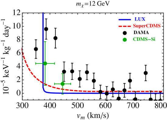
In Fig. 1 we show an example of using the upper bound $\tilde{\eta}_{\rm bnd}(v_{m})$ obtained from null results of the LUX [15] and SuperCDMS [16] experiments to constrain the excess of events observed by CDMS-Si [9], and the annual modulation signal observed by the DAMA experiment [3]. Here we assume spin-independent interactions and a DM mass of 12 GeV.

The black data points and error bars in Fig. 1 show $\tilde{A}_{\eta}^{\rm obs}$ and its corresponding error bars for DAMA obtained from Eq. (4.6). For CDMS-Si we consider two energy bins of 3 keV width in the range of $[7,10]$ and $[10,13]$ keV, containing two and one observed events, respectively. The green data points and error bars in Fig. 1 show $\langle\tilde{\eta}\rangle$ and its corresponding error bars for CDMS-Si obtained from Eq. (4.4) for the two bins. It is clear from Fig. 1 that the upper bounds from LUX and SuperCDMS are in tension with the modulation signal from DAMA and to some extent also with the excess of events observed in CDMS-Si for $m_{\chi}=12$ GeV. While in the case of DAMA the situation is rather clear, indicating conflict at very high CL, for CDMS-Si a more quantitative way of reporting agreement or disagreement is needed. In the following we will provide methods for this purpose.

5 Joint probability of positive and negative results

5.1 Experiments observing excess of events

In this subsection we focus on the case in which an experiment observes an excess of events above their background, such as the case of CDMS-Si. We provide two methods for quantifying the disagreement between the observed excess of events by experiment A and the rate from null-result experiment B, one using only total event numbers and the other using in addition the energy information.

Let us define $p_{B}$ as the probability to obtain equal or less events than observed by the null-result experiment B for a Poisson mean of $\mu(v_{m})$ as defined in Eq. (4.2), with $p_{B}=1-$CL. Then one can use the upper bound $\tilde{\eta}_{\rm bnd}^{B}(v_{m})$, Eq. (4.3), obtained at a confidence level $1-p_{B}$ from experiment B in Eq. (3.9) to get an upper bound on the predicted number of events in experiment A,

$$N^{{\rm bnd},A}_{[E_{1},E_{2}]}=MTA^{2}\int_{0}^{\infty}dE_{nr}F^{2}(E_{nr})G_{[E_{1},E_{2}]}(E_{nr})\tilde{\eta}_{\rm bnd}^{B}(v_{m}).$$ (5.1)

In order to compute the integral on the r.h.s. of Eq. (5.1), $\tilde{\eta}_{\rm bnd}^{B}(v_{m})$ has to be written as a function of the recoil energy deposited in the detector of experiment A.

In practice, one also has to include the expected number of background events in the upper bound on the predicted number of events. If $\beta_{[E_{1},E_{2}]}^{A}$ is the number of background events expected by experiment A in the energy interval $[E_{1},E_{2}]$, then we have an upper bound on the predicted number of events $N^{{\rm pred},A}_{[E_{1},E_{2}]}\leq\mu_{\rm bnd}^{A}$, where

$$\mu_{\rm bnd}^{A}=N^{{\rm bnd},A}_{[E_{1},E_{2}]}+\beta_{[E_{1},E_{2}]}^{A}\,.$$ (5.2)

Note that $N^{{\rm bnd},A}_{[E_{1},E_{2}]}$ depends on the CL that $\tilde{\eta}_{\rm bnd}^{B}$ is obtained at, and thus it depends on $p_{B}$. In this work we always assume that the expected background is known. The motivation for this is that we are interested in the situation of very few signal events (such as in CDMS-Si) and in this case the statistical errors are larger than the assumed uncertainty in the background.

5.1.1 Method 1 – total number of events

In the first method we only use the information on the total number of observed events in the full energy interval. The probability $p_{A}$ of obtaining $N^{{\rm obs},A}_{[E_{1},E_{2}]}$ events or more by experiment A for a Poisson mean of $\mu_{\rm bnd}^{A}$ is given by

$$p_{A}=e^{-\mu_{\rm bnd}^{A}}\,\sum_{n=N^{{\rm obs},A}}^{\infty}\frac{\left(\mu_{\rm bnd}^{A}\right)^{n}}{n!}\,.$$ (5.3)

The combined probability of obtaining the results of experiment A and experiment B is given by $p_{A}~{}p_{B}$, where $p_{A}$ is a function of the chosen $p_{B}$, see Eqs. (5.1) and (5.2). We can then calculate the largest possible joint probability by maximizing with respect to $p_{B}$:

$$p_{\rm joint}=\max_{p_{B}}\left[p_{A}(p_{B})\,\,p_{B}\right]\,.$$ (5.4)

When applying this method some care has to be taken when choosing the energy intervals of the two experiments. We need to make sure that experiment B provides a limit over the full energy range considered in Eq. (5.1) for experiment A. According to Eq. (3.2), the recoil energies in experiments A and B probing the same $v_{m}$ are related by

$$\frac{E_{A}}{E_{B}}=\frac{m_{B}\,\mu^{2}_{\chi A}}{m_{A}\,\mu^{2}_{\chi B}}\,.$$ (5.5)

If the lower edge of the interval for experiment A, $E_{1}$ in Eq. (5.1), is below the threshold of experiment B (after being translated into experiment A energies according to Eq. (5.5)), no limit can be obtained for the expected number of events for experiment A since $\tilde{\eta}$ is unbounded by experiment B below its threshold. Due to the finite energy resolution of experiment A (included in the function $G_{[E_{1},E_{2}]}(E_{nr})$ in Eq. (5.1)) a bound on $\tilde{\eta}$ is even required below the reconstructed energy $E_{1}$. In our analysis of CDMS-Si we require that $E_{1}$ is equal to (or larger than) the thresholds of SuperCDMS or LUX translated into Si recoil energies according to Eq. (5.5) plus 3 times the energy resolution of CDMS-Si.

In Fig. 2 we show the probability that the excess of events observed by CDMS-Si is compatible with null-results from LUX (dashed blue) and SuperCDMS (dashed red) as a function of WIMP mass. For SuperCDMS we find that the threshold of 1.6 keV corresponds to Si energies which are always smaller than the 7 keV threshold of CDMS-Si (including the energy resolution) for the whole range of DM masses shown in the figure. Hence, in this case we consider the full recoil energy range of $[7,100]$ keV for CDMS-Si. For LUX, however, the threshold of the efficiency at 3 keV translated into Si energies plus 3 times the energy resolution is larger than the 7 keV CDMS-Si threshold for DM masses $m_{\chi}\lesssim 20$ GeV. In this case we set $E_{1}$ in Eq. (5.1) to

$$E_{1}=\frac{m_{\rm Xe}\,\mu^{2}_{\chi\rm Si}}{m_{\rm Si}\,\mu^{2}_{\chi\rm Xe}}(3\,{\rm keV})+3\sigma_{\rm res}\,,$$ (5.6)

where $\sigma_{\rm res}=0.3$ keV is the energy resolution we assume for CDMS-Si. Then, if $E_{1}$ computed in this way is larger than the energy of the first, second, or third event observed in CDMS-Si, we take 2, 1, or 0 observed events in the modified energy range, respectively. This is responsible for the steps observed in the LUX curves in Fig. 2: in the regions $m_{\chi}<10\,{\rm GeV}$, $10\,{\rm GeV}\leq m_{\chi}<14\,{\rm GeV}$, $m_{\chi}\geq 14\,{\rm GeV}$ there are 1, 2, 3 events in the analysis window, respectively.

Figure 2: The probability that the excess of events observed by CDMS-Si is compatible with null-results from LUX (blue) and SuperCDMS (red) as a function of WIMP mass. The dashed and solid curves correspond to Method 1 (Poisson probabilities of total number of events in the full energy range) and Method 2 (including energy information of the events via the “signal length”) of obtaining the joint probability, respectively.

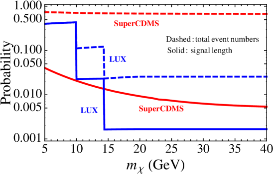
We see that based on this method the joint probability of CDMS-Si and SuperCDMS is around 70%, i.e., signaling essentially compatibility. For CDMS-Si and LUX the joint probability for $m_{\chi}\gtrsim 14$ GeV (where all 3 CDMS-Si events are included in the analysis window) approaches the Poisson probability for the background-only hypothesis, i.e., the probability to obtain 3 or more events for an expectation of 0.62 background events, which is 2.57%. In the following we show that if some information on the energy of the observed events is used, significantly smaller joint probabilities are obtained.

5.1.2 Method 2 – the “signal length” method

In the second method for computing the probability, we use the energy information of the events in addition to the observed number of events. Our method is inspired by the widely used maximum-gap method to set an upper limit [32]. Instead of considering the gap between two events we find it useful to look at the “signal length” (SL), defined in the following way.

Consider an experiment observing $n\geq 2$ events. Then we define the signal length $\Delta$ as

$$\begin{array}[]{rl}\Delta\equiv&\text{expected number of events in the energy interval between}\\ &\text{the two events with the lowest and highest energy.}\end{array}$$ (5.7)

The signal length can be calculated for a given DM model and halo, and includes also the background expectation. Furthermore, let $\mu$ denote the total number of expected events (including background) in the full energy interval for the experiment. Clearly, we have $\Delta\leq\mu$. Suppose experiment A observes $N^{{\rm obs}}$ events. For a given DM model, DM halo, and background, we can calculate the signal length $\Delta$ and the total number of expected events $\mu$ in experiment A. Consider now the probability

$$P(n\geq N^{\rm obs},\,{\rm SL}\leq\Delta|\mu)\equiv P_{\rm SL}(N^{{\rm obs}},\Delta|\mu)\,,$$ (5.8)

i.e., the joint probability of obtaining $N^{{\rm obs}}$ or more events and a signal length of size $\Delta$ or smaller. In App. A.1 we derive the expression for this probability:

$$P_{\rm SL}(N^{{\rm obs}},\Delta|\mu) =e^{-\mu}\sum_{n=N^{{\rm obs}}}^{\infty}\frac{1}{n!}[n\mu\Delta^{n-1}-(n-1)\Delta^{n}]\,.$$ (5.9)

We will use this probability in order to quantify how likely an observation of $N^{{\rm obs}}$ and $\Delta$ is to occur for given $\mu$. It takes into account both the total number of events, as well as some information on the energy distribution of the events. The motivation to consider the signal length is that generically a DM signal is expected to be concentrated in a small energy interval (typically at low energies), whereas background distributions are often more extended. The signal length method is designed to discriminate a signal predicting clustered events from a more broadly distributed background. For instance, we can calculate the probability Eq. (5.9) for the background-only hypothesis in CDMS-Si. In this case, $\mu=0.62$ events (the total background expectation) and $\Delta=0.104$ (integrating the background between 8.2 and 12.3 keV), and we find a probability of $P_{\rm SL}=0.17\%$, which is close to the probability of 0.19% obtained by a likelihood-ratio test between the DM and background only hypotheses [9].

Some comments are in order. Eq. (5.9) is defined only for $N^{\rm obs}\geq 2$. If $\mu\lesssim 2$ the probability becomes small because then it is unlikely to obtain 2 or more events. For $\mu\gtrsim 2$ one has to compare $P_{\rm SL}(N^{{\rm obs}},\Delta|\mu)$ with the value for “typical” outcomes for $N^{{\rm obs}}$ and $\Delta$. In App. A we show that the expectation value of $P_{\rm SL}$ for $\mu\gtrsim 2$ is close to 0.2. Hence we can conclude that if for given $N^{{\rm obs}}$ and $\Delta$ the value of $P_{\rm SL}(N^{{\rm obs}},\Delta|\mu)$ is much smaller than 0.2 those outcomes are quite unlikely, whereas values around 0.2 correspond to a likely outcome. Further discussion of the signal length method is given in the appendix.

In order to apply this method to our case of interest, we need to take into account that we cannot predict $\mu$, but instead have only an upper bound $\mu_{\rm bnd}$. Furthermore, we can calculate an upper bound on the expected number of events in the energy interval between the event with the lowest and highest energy: $\Delta_{\rm bnd}$. Additionally, there may be some background, assumed to be known. Let us denote by $B$ the total number of expected background events and by $b$ the expected background events in the interval between the events with the lowest and highest energies. Hence, the “true” values of $\Delta$ and $\mu$ are bounded as

$$b \leq\Delta\leq\Delta_{\rm bnd},$$ (5.10)

$$\mu_{\rm lo}(\Delta) \leq\mu\leq\mu_{\rm bnd},$$ (5.11)

with

$$\mu_{\rm lo}(\Delta)=B+(\Delta-b)\left[1+\frac{\int_{0}^{\infty}dE_{nr}F^{2}(E_{nr})G_{[E_{1},E_{1}^{\Delta}]}(E_{nr})}{\int_{0}^{\infty}dE_{nr}F^{2}(E_{nr})G_{[E_{1}^{\Delta},E_{2}^{\Delta}]}(E_{nr})}\right]\,.$$ (5.12)

Here $[E_{1},E_{2}]$ is the total energy interval, $[E_{1}^{\Delta},E_{2}^{\Delta}]$ is the interval delimiting the signal length, i.e., $E_{1}^{\Delta}$ and $E_{2}^{\Delta}$ are the energies of the lowest and highest events. In the lower bound for $\mu$ we have taken into account that $\mu$ has to be larger than $\Delta$ plus the background $B-b$ outside the $\Delta$-interval. The second term in the square bracket of Eq. (5.12) follows from the fact that $\tilde{\eta}(v_{m})$ has to be a decreasing function. Then, for a given $\Delta$ there is a lower bound on the expected event rate in the interval $[E_{1},E_{1}^{\Delta}]$ below the signal. Note that $\mu_{\rm bnd}$ and $\Delta_{\rm bnd}$ also include the number of expected background events in the corresponding energy regions, and depend on the CL.

We have to maximize the probability in Eq. (5.9) with respect to $\Delta$ and $\mu$, taking into account the allowed ranges for them. First, it is easy to see that Eq. (5.9) is a monotonously increasing function in $\Delta$. Hence the maximum probability is obtained by setting $\Delta=\Delta_{\rm bnd}$. Second, by differentiating Eq. (5.9) with respect to $\mu$ one finds that it has a maximum for

$$\hat{\mu}=1+\frac{\sum_{n=N^{{\rm obs}}}^{\infty}\frac{n-1}{n!}\Delta^{n}}{\sum_{n=N^{{\rm obs}}}^{\infty}\frac{1}{(n-1)!}\Delta^{n-1}}\,.$$ (5.13)

Now we have to take into account the allowed range for $\mu$ in Eq. (5.11). Hence, in order to maximize the probability we define:

$$\mu_{\rm max}\equiv\left\{\begin{array}[]{l@{\quad\text{for}\quad}l}\mu_{\rm lo}(\Delta_{\rm bnd})&\hat{\mu}<\mu_{\rm lo}(\Delta_{\rm bnd})\\ \hat{\mu}&\mu_{\rm lo}(\Delta_{\rm bnd})\leq\hat{\mu}\leq\mu_{\rm bnd}\\ \mu_{\rm bnd}&\hat{\mu}>\mu_{\rm bnd}\end{array}\right.$$ (5.14)

Now we can use $P_{\rm SL}(N^{{\rm obs}},\Delta_{\rm bnd}|\mu_{\rm max})$ to check how likely a given outcome is even if only an upper bound on the event rate is available.

In order to use the signal length probability to evaluate the joint probability of experiment A (seeing a signal) and experiment B (giving a limit) we proceed as follows. We specify the probability for experiment B, $p_{B}$, and calculate an upper bound on the halo integral $\tilde{\eta}_{\rm bnd}^{B}(v_{m})$ from Eq. (4.3) at the confidence level CL $=1-p_{B}$. This bound is then used in Eqs. (5.1) and (5.2) to calculate the upper bounds $\mu_{\rm bnd}$ and $\Delta_{\rm bnd}$ for experiment A, by using in those equations for the energy interval $[E_{1},E_{2}]$ either the total energy interval of the experiment (for $\mu_{\rm bnd}$) or the energy interval between the events with smallest and largest energies (for $\Delta_{\rm bnd}$). Then we can calculate $P_{\rm SL}(N^{{\rm obs}},\Delta_{\rm bnd}|\mu_{\rm max})$ for that particular choice of $p_{B}$. As before, we maximize with respect to $p_{B}$ to obtain the maximal joint probability for the combined result:

$$p_{\rm joint}=\max_{p_{B}}\left[P_{\rm SL}(N^{{\rm obs}},\Delta_{\rm bnd}|\mu_{\rm max})~{}p_{B}\right]\,.$$ (5.15)

The solid blue and red curves in Fig. 2 show the results of such an analysis for the compatibility between the signal in CDMS-Si and the null-results of LUX and SuperCDMS, respectively. We find significantly smaller probabilities than in the case of using total event numbers only (dashed curves), illustrating the importance of using energy information and the power of the signal length test. The joint probability of CDMS-Si and SuperCDMS is 4% for $m_{\chi}\simeq 5$ GeV, decreasing to 0.5% for $m_{\chi}\simeq 40$ GeV. For LUX we proceed as before, taking as energy threshold the maximum of the threshold energies of the two experiments, after equalizing them via the $v_{m}$ method, see Eq. (5.6). The step-like structure of the probability emerges from the fact that when decreasing the DM mass, the Si-equivalent energy of the LUX threshold is increasing. The steps occur when the threshold passes the energies of the observed events. For $m_{\chi}\lesssim 10$ GeV only one event is left in the analysis window and the signal-length method can no longer be applied (since it is defined only for $\geq 2$ events). In this case we use method 1, calculating just the Poisson probability to obtain one event, which essentially provides no constraint given the expected background. On the other hand, for $m_{\chi}\gtrsim 14$ GeV, when all three events are inside the analysis interval, we find joint probabilities very close to the probability of the background only hypothesis for CDMS-Si of 0.17%, which is the maximal possible rejection CL of the signal.

5.2 Experiments observing annual modulation

Let us now show how to quantify the disagreement between an experiment A observing an annual modulation signal and a null-result experiment B providing an upper limit on the unmodulated rate [22]. We first consider the trivial bound given in Eq. (4.7), demanding that the amplitude of the modulation is smaller than the bound on the unmodulated rate. We calculate the probability $p_{B}$ to obtain equal or less events than observed by the null-result experiment B for each value of $\tilde{\eta}_{\rm bnd}^{B}(v_{m})$. Using the same value of $\tilde{\eta}_{\rm bnd}^{B}(v_{m})$ on the r.h.s. of Eq. (4.7), we calculate the probability $p_{A}$ to obtain a value of the modulation amplitude in a fixed energy bin equal to or larger than the observed one, assuming a Gaussian distribution for it, with a mean given by $\tilde{\eta}_{\rm bnd}^{B}(v_{m})$ and a standard deviation given by the experimental error on the modulation amplitude. Hence, for a given energy bin $i$ we have

$$p_{A}=\frac{1}{2}\left[1-\operatorname{erf}\left(\frac{\tilde{A}^{\rm obs}_{\eta}(v_{m}^{i})-\tilde{\eta}_{\rm bnd}^{B}(v_{m}^{i})}{\sqrt{2}\,\sigma_{\tilde{A}}(v_{m}^{i})}\right)\right],$$ (5.16)

where $\sigma_{\tilde{A}}(v_{m}^{i})$ is the experimental error on $\tilde{A}^{\rm obs}_{\eta}$ in bin $i$. The joint probability of obtaining the experimental result for a fixed value of $\tilde{\eta}_{\rm bnd}^{B}$ is given by $p_{A}(p_{B})~{}p_{B}$, and the highest possible joint probability is obtained by maximizing with respect to $p_{B}$:

$$p_{\rm joint}=\max_{p_{B}}\left[p_{A}(p_{B})~{}p_{B}\right].$$ (5.17)

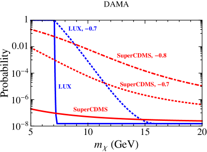
As an example, we apply our method to the case of the DAMA annual modulation signal. We perform the analysis at a fixed $v_{m}$ which corresponds to the center of the 3rd modulation data point in DAMA and depends on the DM mass. This choice is arbitrary, but motivated by Fig. 1, which suggests strong tension around the $v_{m}$ corresponding to the 3rd bin. The probability that the DAMA modulation amplitude in that bin is compatible with the constraints on $\tilde{\eta}$ from LUX and SuperCDMS is shown by solid blue and red curves in Fig. 3, respectively, indicating very strong tension between the results. From Fig. 3, one can see a sharp increase in the probability for LUX at low masses. Again this sharp cut-off is due to setting the LUX detection efficiency equal to zero below $E_{nr}=3$ keV. This results in having no upper bound on $\tilde{\eta}$ at small DM masses ($\leq 7$ GeV), when the minimal velocity threshold (corresponding to 3 keV recoil energy) in LUX becomes larger than the $v_{m}$ corresponding to the energy of the 3rd modulation data point in DAMA.

Figure 3: The probability that the modulation amplitude in DAMA is compatible with the null-results from LUX (blue curves) and SuperCDMS (red curves). The solid curves correspond to the trivial bound, requiring that the modulation amplitude is less than the bound on the unmodulated rate. $v_{m}$ is fixed at a value corresponding to the 3rd modulation data point in DAMA. The dashed curves correspond to the bound based on the expansion in $v_{e}$, Eq. (5.18). The integration of the modulation amplitude starts from the 3rd bin in DAMA.

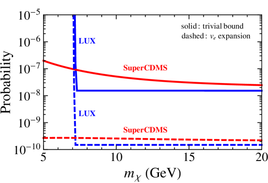
In Refs. [31, 22] it has been shown that under certain regularity assumptions on the DM halo a much stronger bound on the modulation amplitude can be obtained by expanding the halo integral in the small Earth’s velocity $v_{e}$. Under the assumption that the DM velocity distribution in the Sun’s rest frame is constant in time on the scale of 1 year and in space on the scale of the size of the Sun–Earth distance, the modulation amplitude is bounded as

$$\int_{v_{1}}^{v_{2}}dv_{m}\tilde{A}_{\eta}^{\rm obs}(v_{m})\leq v_{e}\left[\tilde{\eta}_{\rm bnd}(v_{1})+\int_{v_{1}}^{v_{2}}dv\frac{\tilde{\eta}_{\rm bnd}(v)}{v}\right]\,.$$ (5.18)

We can compute the disagreement between the observed annual modulation signal in one experiment and the rate from another experiment in a way similar to that of the trivial bound, except that for the bound in Eq. (5.18) we calculate $p_{A}$ by assuming a Gaussian distribution on the l.h.s. of Eq. (5.18), and for the integral on the r.h.s. of Eq. (5.18) we take the bound $\tilde{\eta}_{\rm bnd}(v_{m})$ at constant probability $p_{B}$.

We apply our method for the bound in Eq. (5.18) to the case of DAMA. For the lower and upper integration limits, $v_{1}$ and $v_{2}$ in Eq. (5.18), we take the $v_{m}$ corresponding to the beginning of the 3rd and the end of the 12th bins in DAMA, respectively. Above the 12th energy bin (i.e. above 8 keVee), the data is consistent with no modulation. The dashed blue and red curves in Fig. 3 show the probability that the integrated modulation amplitude in DAMA is compatible with the bound (r.h.s. of Eq. (5.18)) derived from constraints on $\tilde{\eta}$ from LUX and SuperCDMS, respectively. As expected, the bound based on the expansion in $v_{e}$ is a few orders of magnitude stronger than the trivial bound, and thus the compatibility between the DAMA signal and the results from LUX and SuperCDMS becomes weaker for the $v_{e}$ expansion bound compared to the trivial bound. A similar analysis has been performed in Ref. [22] also for different experiments and different DM–nucleus interactions, such as spin-dependent interactions and interactions with arbitrary couplings to protons and neutrons.

6 Isospin violating interactions

In the previous sections we assumed the so-called isospin conserving DM-nucleon interaction, i.e. that DM couples with the same strength to protons and neutrons, such that $f_{n}=f_{p}$. However, in general this assumption does not need to be satisfied, e.g. [41, 42]. In particular, in the case of a relative sign between $f_{n}$ and $f_{p}$ there could be a suppression factor for the spin-independent DM-nucleus cross section (see Eq. (3.4)) due to a cancellation between the contributions from neutrons and protons, depending on the target element of the experiment. Since this can have important consequences for the compatibility of different experiments, in this section we consider a few interesting cases in which $f_{n}\neq f_{p}$.

Figure 4: The probability that the excess of events observed by CDMS-Si using the signal length method (left panel) or the modulation amplitude in DAMA using the trivial bound at the 3rd modulation data point (right panel) is compatible with null-results from LUX (blue) and SuperCDMS (red). The solid curves correspond to isospin conserving interactions, whereas the dotted and dot-dashed curves correspond to isospin violating interactions with $f_{n}/f_{p}=-0.7$ and $-0.8$, respectively. The LUX curve for $f_{n}/f_{p}=-0.8$ coincides with the isospin conserving curve (solid).

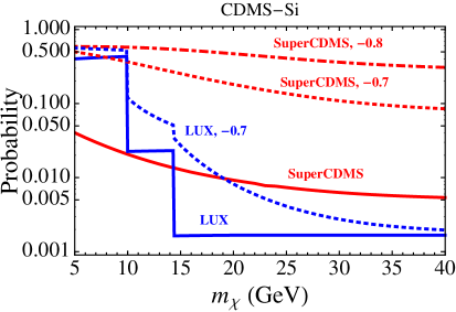
We take into account the natural abundances of the isotopes present in each detector to compute the cross section, but neglect the effect of different isotopes on the form factors and kinematics. The cross section reaches a minimum at $f_{n}/f_{p}\simeq-0.7$ and $-0.8$ for Xe and Ge, respectively (see the left panel of Fig. 5 in [43]). Since for those values of $f_{n}/f_{p}$, the cross section is not highly suppressed for Si and Na, the compatibility between CDMS-Si/DAMA and LUX/SuperCDMS can be improved. A comparison of the joint probabilities for the isospin conserving and isospin violating cases is shown in Fig. 4. In the left panel we show the joint probability of obtaining the positive CDMS-Si result and the negative LUX and SuperCDMS results, using the signal length method. In the right panel, the joint probability of obtaining the DAMA modulation signal and the null results from LUX and SuperCDMS is shown, using the trivial bound at a fixed $v_{m}$ corresponding to the 3rd modulation data point in DAMA. Clearly, assuming a value of $f_{n}/f_{p}$ which suppresses the cross section for Xe and Ge, leads to a higher joint probability. In the figure we assume $f_{n}/f_{p}=-0.7$ and $-0.8$, which maximally suppresses the cross section for Xe and Ge, respectively. For LUX, the cross section is not suppressed by much at $f_{n}/f_{p}=-0.8$ and the curves for that case coincide with the isospin conserving curves.

We find that the signal in CDMS-Si essentially becomes consistent with SuperCDMS for $f_{n}/f_{p}=-0.8$, while it is inconsistent with LUX for $m_{\chi}\gtrsim 14$ as in the isospin conserving case. For $f_{n}/f_{p}=-0.7$, the joint probability of CDMS-Si and SuperCDMS decreases to 18% for $m_{\chi}\simeq 20$ GeV, and the joint probability with LUX remains below 1% for $m_{\chi}\geq 19$ GeV. For DAMA the compatibility with LUX for $f_{n}/f_{p}=-0.7$ and with SuperCDMS for $f_{n}/f_{p}=-0.8$ is increased by many orders of magnitude for $m_{\chi}\lesssim 10$ GeV compared to the isospin conserving case ($p_{\rm joint}\gtrsim 1\%$). However the compatibility of DAMA cannot be improved considerably with both LUX and SuperCDMS for a fixed choice of $f_{n}/f_{p}$. For example, for $f_{n}/f_{p}=-0.7$ the joint probability of DAMA and SuperCDMS always remains below 1%. Let us also note that for a given value of $f_{n}/f_{p}$, other data not considered here may still be in considerable tension with DAMA. Furthermore, using the bound based on the $v_{e}$ expansion (Eq. (5.18)) stronger limits can be obtained also in the isospin violating case. For instance, in Ref. [22] it was shown that for $f_{n}/f_{p}=-0.7$ data from the CDMS silicon target [46] leads to joint probabilities with DAMA between $10^{-7}$ and $10^{-4}$ for DM masses between 5 and 20 GeV.

7 Summary and discussion

In the interpretation of results from DM direct detection experiments, uncertainties related to the local DM distribution are crucial. The so-called $v_{m}$ method allows for a completely halo independent comparison of different experiments by considering constraints in terms of the halo integral $\tilde{\eta}(v_{m})$. Starting from this idea, we have presented a method to evaluate the joint probability of obtaining the outcomes of two potentially conflicting experiments, under the assumption that the DM hypothesis is true. This allows a quantitative assessment of the compatibility of such results.

The main idea is the following. For a given value of $\tilde{\eta}(v_{m})$ we calculate the probabilities $p_{A}$ and $p_{B}$ of obtaining the outcomes of the two experiments A and B, respectively. The joint probability is just given by the product $(p_{A}p_{B})$. Then we report the maximal possible joint compatibility by maximizing this product with respect to $\tilde{\eta}(v_{m})$. For technical reasons it turns out to be practical to consider $p_{A}$ as a function of $p_{B}$ and maximize $(p_{A}p_{B})$ with respect to $p_{B}$, as described in detail in section 5.

We have illustrated the method by comparing the positive indications for DM scattering from CDMS-Si and the annual modulation in DAMA with the limits from the LUX and SuperCDMS experiments. For DAMA we confirm previous results [22] and we obtain very low joint probabilities of $p_{\rm joint}\lesssim 10^{-7}$ for SuperCDMS and $p_{\rm joint}\simeq 10^{-8}$ for LUX.

In the case of CDMS-Si we face the situation that the signal itself is rather weak, consisting of only 3 events with an expected background of 0.62 events. When only the information of the number of events is used the CL for a signal being present is very low (around 97.4%), and hence a possible exclusion of the signal from other experiments is possible at best at the same very modest CL. For this reason we have identified a method to take into account energy information. An important observation is that the three events cluster at relatively low energies, as expected from a DM signal, compared to the more broadly distributed background. Therefore, we consider the so-called signal length, defined as the expected number of events in the energy interval between the events with the lowest and highest energies. We can calculate the probability of obtaining a signal length equal or less than the one obtained in CDMS-Si and use it to get the joint probability with constraints from LUX and SuperCDMS. We find CDMS-Si and SuperCDMS being consistent with a probability of 4% for $m_{\chi}\simeq 5$ GeV, decreasing to 0.5% for $m_{\chi}\simeq 40$ GeV. For $m_{\chi}\gtrsim 14$ GeV, LUX provides a strong bound leading to a joint probability basically given by the probability of the background only hypothesis of 0.17%.

We have also applied our method to the case of isospin violating interactions, where for a specific choice of the DM coupling strengths to neutrons and protons the scattering cross section of the experiments providing upper limits can be significantly suppressed relative to the one relevant for the experiment reporting a signal. For Xe (Ge) the maximum suppression occurs for $f_{n}/f_{p}=-0.7$ ($-0.8$). A careful choice of $f_{n}/f_{p}$ allows for better compatibility of CDMS-Si with LUX and SuperCDMS (at relatively small DM masses), whereas for DAMA for any $f_{n}/f_{p}$ the joint probability with at least one of the other experiments remains small.

The signal length method used in this work to take into account energy information is one particular observable which turns out to be useful to test the CDMS-Si signal. It is inspired by the popular maximum-gap method [32], and in addition to the total number of events it takes into account a second observable (the “signal length”) given by the properly defined distance between the two events with the lowest and highest energy. It has the advantage that the relevant probability can be analytically calculated and is relatively simple, see Eq. (5.9). The signal length method provides a goodness-of-fit test returning a probability for the actual experimental outcome to occur under a given hypothesis. It is useful in the case of signals consisting of few (but at least two) events. Further discussion of the method can be found in App. A. While the signal length turns out to be powerful in the case of CDMS-Si we do not exclude the possibility that in other situations different observables might also be identified and used in a similar fashion as the signal length.

Let us stress that the probabilities obtained by our method are actually upper bounds on the joint probability. In several steps in our calculations we use inequalities or maximization, for instance in Eq. (4.1) to set an upper bound on the halo integral, in calculating the relevant probability for the signal length in section 5.1.2, or in maximizing the joint probability $p_{A}p_{B}$ in Eqs. (5.4) or (5.15). The true probability of obtaining the two experimental results will actually be lower than the value returned by our method.

Let us briefly compare our results to the ones obtained by Feldstein and Kahlhoefer in Ref. [34]. They consider the joint likelihood function for CDMS-Si, SuperCDMS, and LUX, optimized with respect to all possible DM halo configurations and the DM mass. In addition a constraint on the galactic escape velocity is imposed in their likelihood. They obtain a best fit DM mass of 5.7 GeV and determine the p-value of the fit by Monte Carlo method as 0.44%. From our Fig. 2 we find at $m_{\chi}=5.7$ GeV a joint probability of CDMS-Si and SuperCDMS of 3.6%, whereas the LUX constraint is absent at those low DM masses. We stress that the approaches are quite different, leading to different statistical statements. Hence a direct quantitative comparison is difficult. The likelihood method uses a maximum of information from each event, so even the single event tested by LUX for $m_{\chi}=5.7$ GeV provides some constraint. Our method uses energy information in a more condensed way (via the signal length) and is more conservative in several respects. It has the advantage of providing directly a probability for how likely the experimental outcome is under the DM hypothesis, without the need of Monte Carlo simulations.

Acknowledgements

We thank Brian Feldstein and especially Felix Kahlhoefer for comments on the manuscript and very useful discussions. We acknowledge support from the European Union FP7 ITN INVISIBLES (Marie Curie Actions, PITN-GA-2011-289442). N.B. thanks the Oskar Klein Centre and the CoPS group at the University of Stockholm for hospitality during her long-term visit.

Appendix A The signal length method

In this appendix we provide some details on the signal length method. In App. A.1 we derive the joint probability $P_{\rm SL}(N^{{\rm obs}},\Delta|\mu)$ from Eq. (5.9) of obtaining $N^{{\rm obs}}$ or more events and a signal length of size $\Delta$ or smaller. We discuss some properties of the SL test in App. A.2, where we also demonstrate that the SL method can be used to obtain allowed regions in DM mass and scattering cross section if a specific halo is adopted for the example of the CDMS-Si data. A general discussion of the method follows in Sec. A.3.

A.1 Probability derivation

Let us denote by $dN/dE_{nr}$ the expected event spectrum for a given DM model, DM halo, and background. The expected number of events between two energies $E_{1}$ and $E_{2}$ is then given by

$$N_{[E_{1},E_{2}]}=\int_{E_{1}}^{E_{2}}dE_{nr}\,\frac{dN}{dE_{nr}}\,.$$ (A.1)

The value of $N_{[E_{1},E_{2}]}$ is invariant under a change of variable. In particular, we can always use a new variable $x$ with $dx=dN$, such that the distribution of $x$ is constant and equal to unity in the interval $[0,\mu]$, where $\mu$ is the expected number of events in the total energy interval [32]. The expected number of events in a given energy interval is simply $N_{[E_{1},E_{2}]}=x_{2}-x_{1}$.

Hence the problem reduces to the following. Assume $n$ independent random numbers $x_{n}$, uniformly distributed in the interval $[0,\mu]$. We order the events as $x_{1}<x_{2}<...<x_{n}$. The “signal length” is then given by $\Delta=x_{n}-x_{1}$. We want to calculate the probability of obtaining a signal length less than $\Delta$ for given $n$, $P({\rm SL}<\Delta|n)=1-P({\rm SL}\geq\Delta|n)$. We calculate $P({\rm SL}\geq\Delta|n)$ as (probability of $x_{1}\in[0,\mu-\Delta]$) times (probability of $x_{n}\in[x_{1}+\Delta,\mu]$) times (probability of all $x_{2},...,x_{n-1}$ between $x_{1}$ and $x_{n}$) times a combinatorial factor:

$$P({\rm SL}\geq\Delta|n)=2\left(\begin{array}[]{c}n\\ 2\end{array}\right)\frac{1}{\mu^{n}}\int_{0}^{\mu-\Delta}dx_{1}\int_{x_{1}+\Delta}^{\mu}dx_{n}\,(x_{n}-x_{1})^{n-2}\,.$$ (A.2)

The binomial coefficient

$$\left(\begin{array}[]{c}n\\ 2\end{array}\right)=\frac{n!}{(n-2)!2!}=\frac{n(n-1)}{2}$$ (A.3)

corresponds to the number of possibilities to pick $2$ events out of $n$ (the ones we call $x_{1}$ and $x_{n}$), and the factor 2 is needed because of the two possibilities of either of them being the smaller or the larger. The factor $1/\mu^{n}$ ensures that the probability of finding each event between 0 and $\mu$ is normalized to 1. The integrals are easily calculated and we find

$$P({\rm SL}<\Delta|n)=1-P({\rm SL}\geq\Delta|n)=n\left(\frac{\Delta}{\mu}\right)^{n-1}-(n-1)\left(\frac{\Delta}{\mu}\right)^{n}\,.$$ (A.4)

The corresponding probability distribution function (pdf) for the signal length $\Delta$ is obtained by differentiating Eq. (A.4) as

$$f(\Delta|n)=n(n-1)\frac{1}{\mu}\left(\frac{\Delta}{\mu}\right)^{n-2}\left(1-\frac{\Delta}{\mu}\right)\,,$$ (A.5)

which is defined for $n\geq 2$ and $\Delta\leq\mu$.

The joint pdf for the number of events $n$ and the signal length $\Delta$ for a given $\mu$ is obtained from Bayes’ theorem as

$$f(n,\Delta)=f(\Delta|n)f(n)=\frac{1}{(n-2)!}\,e^{-\mu}\Delta^{n-2}(\mu-\Delta)\,.$$ (A.6)

We have used that $n$ is Poisson distributed with mean $\mu$, and $f(n,\Delta)$ is defined for $n\geq 2$ and $\Delta\leq\mu$. The normalization is such that

$$\sum_{n=2}^{\infty}\int_{0}^{\mu}d\Delta f(n,\Delta)=\mathcal{P}_{\mu}(n\geq 2)\,,$$ (A.7)

where $\mathcal{P}_{\mu}(n\geq 2)=1-e^{-\mu}(1+\mu)$ is the Poisson probability for obtaining $n\geq 2$ for Poisson mean $\mu$. Hence the normalized pdf is given by

$$\tilde{f}(n,\Delta)\equiv\frac{f(n,\Delta)}{\mathcal{P}_{\mu}(n\geq 2)}\,.$$ (A.8)

It describes the distribution of $n$ and $\Delta$ given that $n\geq 2$ events have been observed.

Suppose an experiment observes $N^{\rm obs}$ events. Then the joint probability to obtain a number of events equal or larger than $N^{\rm obs}$ and a signal length equal or smaller than $\Delta$ for a given $\mu$ is

$$P_{\rm SL}(N^{\rm obs},\Delta|\mu) =\sum_{n=N^{{\rm obs}}}^{\infty}\int_{0}^{\Delta}d\Delta^{\prime}f(n,\Delta^{\prime})$$ (A.9)

$$=e^{-\mu}\sum_{n=N^{{\rm obs}}}^{\infty}\frac{1}{n!}[n\mu\Delta^{n-1}-(n-1)\Delta^{n}]\,.$$ (A.10)

Eq. (A.10) corresponds to the expression in Eq. (5.9) used in our analysis of DM direct detection data.

A.2 Properties of the SL and application to CDMS-Si data

Using the normalized pdf, Eq. (A.8), we can calculate the expectation value of any quantity $X$ which depends on the random variables $n$ and $\Delta$:

$$\langle X\rangle=\sum_{n=2}^{\infty}\int_{0}^{\mu}d\Delta\,X\,\tilde{f}(n,\Delta)\,.$$ (A.11)

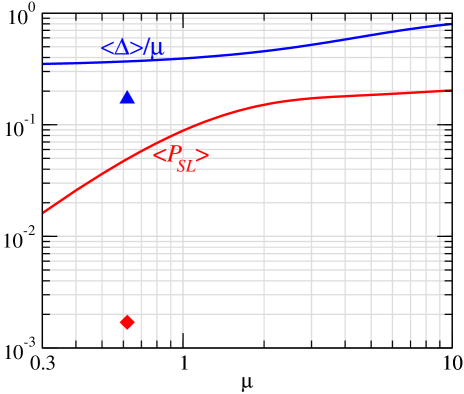
For instance we can calculate the expected value of the signal length $\Delta$. The blue curve in Fig. 5 shows $\langle\Delta\rangle/\mu$ as a function of the expected number of events $\mu$. The probability $P_{\rm SL}$ will be small if a SL much smaller than $\langle\Delta\rangle$ is observed. The blue triangle shows the value of $\Delta/\mu$ corresponding to the background-only hypothesis of CDMS-Si, with $\Delta=0.104$ and $\mu=0.62$.

Figure 5: Expectation values of the signal length $\langle\Delta\rangle/\mu$ and of the signal length probability $\langle P_{\rm SL}\rangle$ as a function of $\mu$. The blue triangle and the red diamond indicate the values of $\Delta/\mu$ and $P_{\rm SL}$, respectively, obtained for the background-only hypothesis for CDMS-Si for which $\Delta=0.104$ and $\mu=0.62$.

We can use Eq. (A.11) to calculate also the expected value of $P_{\rm SL}$ itself, considered as a function of $\Delta$ and $n$:

$$\langle P_{\rm SL}\rangle=\sum_{n=2}^{\infty}\int_{0}^{\mu}d\Delta\,P_{\rm SL}(n,\Delta|\mu)\,\tilde{f}(n,\Delta)\,.$$ (A.12)

This is shown by the red curve in Fig. 5. We observe that for $\mu\lesssim 2$ we expect that $P_{\rm SL}$ becomes small, because it is unlikely to obtain at least 2 events. For $\mu\gtrsim 2$ we find $\langle P_{\rm SL}\rangle\simeq 0.2$. Hence, whenever the observed value for $P_{\rm SL}$ is much smaller than 0.2 the experimental outcome can be considered to be unlikely. The red diamond in Fig. 5 indicates the value $P_{\rm SL}=0.17\%$ obtained for the background-only hypothesis for CDMS-Si, which is significantly smaller than the expectation.

If on top of the backgrounds a specific DM hypothesis is specified, the SL method provides a way to quantify how likely the experimental outcome is under this hypothesis. In Fig. 6 we show the results of such an analysis for CDMS-Si data, assuming spin-independent elastic DM–nucleon interactions and the so-called standard halo model for the local DM velocity distribution. Then, for each point in the plane of DM mass and scattering cross section we can calculate $\mu$, the SL $\Delta$, and $P_{\rm SL}$. The black curves in the figure show contours of constant values of $P_{\rm SL}$ between 0.01 and 0.25. The black dot indicates the point of highest probability, which is $P_{\rm SL}=0.266$, i.e., close to the expectation value (compare to Fig. 5).

Figure 6: Regions in the plane of DM mass and scattering cross section from CDMS-Si data assuming the so-called standard halo model. The black curves show equal probability contours using the signal length method corresponding to $P_{\rm SL}=0.01,0.05,0.1,0.2,0.25$, from outer to inner contours. The black dot indicates the point of highest probability. The shaded regions (black triangle) correspond to 68% and 90% CL regions (best fit point) using an extended maximum likelihood analysis.

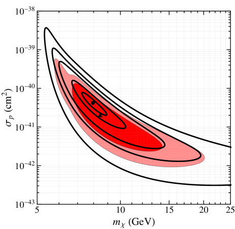
The contours of constant $P_{\rm SL}$ can be compared to more traditional regions obtained from an extended maximum likelihood analysis of CDMS-Si data, shown by the shaded regions in Fig. 6. This analysis is similar to the ones performed in [47, 27] and leads to allowed regions in good agreement with the ones obtained by the CDMS-Si collaboration [9]. We observe very good agreement of the regions between the two methods, although we stress the different meanings. The SL method provides regions where the experimental outcome is likely (in the sense of a goodness-of-fit test), while the maximum likelihood method leads to confidence regions in the parameter space under the hypothesis that the DM interpretation is correct (i.e., regions relative to the best fit point).

A.3 Discussion

The SL method can be used to quantify how likely a given experimental outcome is for a specified hypothesis. It works well for low event numbers (but at least 2 events are needed). It is based on the predicted number of events between the energy of the lowest and highest event (the “signal length” $\Delta$) as well as on the predicted number of events in the full energy range $\mu$. In some sense the SL method is based on two “bins”, the total energy interval and the one between the lowest and highest event. The size of the $\Delta$ bin is determined by the data and it is actually the bin size which contains the relevant information used to calculate the probability. The full probability distribution of the expected events has to be known to calculate $\Delta$ and $\mu$, similar to the case of a likelihood analysis. While the SL method provides a goodness-of-fit test, returning an absolute probability, a maximum likelihood analysis is based on the relative likelihood of parameter points with respect to the best fit point (assuming that the model itself is correct).

The SL method is powerful in the case of few events to evaluate signal versus background-only hypotheses which have a distinct energy shape, for instance a peaked signal versus a broader distribution of background. The method becomes not very useful in case of many events. In this case the two numbers $\Delta$ and $\mu$ provide only limited information on the detailed event spectrum and in such a case alternative methods will be more powerful, for example binned $\chi^{2}$ goodness-of-fit, un-binned Kolmogorov-Smirnov shape test, or likelihood ratio tests.

The relevant probability $P_{\rm SL}$ for the SL test has a relatively simple expression, see Eq. (A.10), which can easily be evaluated numerically. Thanks to this simple form and the fact that $P_{\rm SL}$ depends only on $\Delta$ and $\mu$, the SL method is also useful if the hypothesis is constrained by other data or consistency requirements. Maximization with respect to $\Delta$ and $\mu$ provides then an upper bound on the probability, as demonstrated explicitly in Sec. 5.1.2. Similar methods may be used also to take into account uncertainties in the predicted spectrum, for instance uncertainty on the expected background.

References

- [1] M. W. Goodman and E. Witten, Detectability of Certain Dark Matter Candidates, Phys.Rev. D31, 3059 (1985).
- [2] DAMA/LIBRA Collaboration, R. Bernabei et al., New results from DAMA/LIBRA, Eur.Phys.J. C67, 39 (2010), 1002.1028.
- [3] R. Bernabei et al., Final model independent result of DAMA/LIBRA-phase1, Eur.Phys.J. C73, 2648 (2013), 1308.5109.
- [4] CoGeNT, C. E. Aalseth et al., Results from a Search for Light-Mass Dark Matter with a P- type Point Contact Germanium Detector, Phys. Rev. Lett. 106, 131301 (2011), 1002.4703.
- [5] C. E. Aalseth et al., Search for an Annual Modulation in a P-type Point Contact Germanium Dark Matter Detector, (2011), 1106.0650.
- [6] CoGeNT Collaboration, C. Aalseth et al., CoGeNT: A Search for Low-Mass Dark Matter using p-type Point Contact Germanium Detectors, Phys.Rev. D88, 012002 (2013), 1208.5737.
- [7] CoGeNT Collaboration, C. Aalseth et al., Search for An Annual Modulation in Three Years of CoGeNT Dark Matter Detector Data, (2014), 1401.3295.
- [8] G. Angloher et al., Results from 730 kg days of the CRESST-II Dark Matter Search, Eur.Phys.J. C72, 1971 (2012), 1109.0702.
- [9] CDMS Collaboration, R. Agnese et al., Silicon Detector Dark Matter Results from the Final Exposure of CDMS II, Phys.Rev.Lett. 111, 251301 (2013), 1304.4279.
- [10] CDMS-II Collaboration, Z. Ahmed et al., Dark Matter Search Results from the CDMS II Experiment, Science 327, 1619 (2010), 0912.3592.
- [11] CDMS-II, Z. Ahmed et al., Results from a Low-Energy Analysis of the CDMS II Germanium Data, Phys. Rev. Lett. 106, 131302 (2011), 1011.2482.
- [12] XENON10 Collaboration, J. Angle et al., A search for light dark matter in XENON10 data, Phys.Rev.Lett. 107, 051301 (2011), 1104.3088.
- [13] XENON100 Collaboration, E. Aprile et al., Dark Matter Results from 225 Live Days of XENON100 Data, Phys.Rev.Lett. 109, 181301 (2012), 1207.5988.
- [14] S. Kim et al., New Limits on Interactions between Weakly Interacting Massive Particles and Nucleons Obtained with CsI(Tl) Crystal Detectors, Phys.Rev.Lett. 108, 181301 (2012), 1204.2646.
- [15] LUX Collaboration, D. Akerib et al., First results from the LUX dark matter experiment at the Sanford Underground Research Facility, Phys.Rev.Lett. 112, 091303 (2014), 1310.8214.
- [16] SuperCDMS Collaboration, R. Agnese et al., Search for Low-Mass WIMPs with SuperCDMS, Phys.Rev.Lett. 112, 241302 (2014), 1402.7137.
- [17] P. J. Fox, J. Liu, and N. Weiner, Integrating Out Astrophysical Uncertainties, Phys.Rev. D83, 103514 (2011), 1011.1915.
- [18] P. J. Fox, G. D. Kribs, and T. M. Tait, Interpreting Dark Matter Direct Detection Independently of the Local Velocity and Density Distribution, Phys.Rev. D83, 034007 (2011), 1011.1910.
- [19] C. McCabe, DAMA and CoGeNT without astrophysical uncertainties, Phys.Rev. D84, 043525 (2011), 1107.0741.
- [20] M. T. Frandsen, F. Kahlhoefer, C. McCabe, S. Sarkar, and K. Schmidt-Hoberg, Resolving astrophysical uncertainties in dark matter direct detection, JCAP 1201, 024 (2012), 1111.0292.
- [21] P. Gondolo and G. B. Gelmini, Halo independent comparison of direct dark matter detection data, JCAP 1212, 015 (2012), 1202.6359.
- [22] J. Herrero-Garcia, T. Schwetz, and J. Zupan, Astrophysics independent bounds on the annual modulation of dark matter signals, Phys.Rev.Lett. 109, 141301 (2012), 1205.0134.
- [23] N. Bozorgnia, J. Herrero-Garcia, T. Schwetz, and J. Zupan, Halo-independent methods for inelastic dark matter scattering, JCAP 1307, 049 (2013), 1305.3575.
- [24] E. Del Nobile, G. Gelmini, P. Gondolo, and J.-H. Huh, Generalized Halo Independent Comparison of Direct Dark Matter Detection Data, JCAP 1310, 048 (2013), 1306.5273.
- [25] E. Del Nobile, G. B. Gelmini, P. Gondolo, and J.-H. Huh, Halo-independent analysis of direct detection data for light WIMPs, (2013), 1304.6183.
- [26] E. Del Nobile, G. B. Gelmini, P. Gondolo, and J.-H. Huh, Update on Light WIMP Limits: LUX, lite and Light, JCAP 1403, 014 (2014), 1311.4247.
- [27] M. T. Frandsen, F. Kahlhoefer, C. McCabe, S. Sarkar, and K. Schmidt-Hoberg, The unbearable lightness of being: CDMS versus XENON, JCAP 1307, 023 (2013), 1304.6066.
- [28] P. J. Fox, Y. Kahn, and M. McCullough, Taking Halo-Independent Dark Matter Methods Out of the Bin, (2014), 1403.6830.
- [29] B. Feldstein and F. Kahlhoefer, A new halo-independent approach to dark matter direct detection analysis, JCAP 1408, 065 (2014), 1403.4606.
- [30] J. F. Cherry, M. T. Frandsen, and I. M. Shoemaker, Halo Independent Direct Detection of Momentum-Dependent Dark Matter, JCAP 1410, 022 (2014), 1405.1420.
- [31] J. Herrero-Garcia, T. Schwetz, and J. Zupan, On the annual modulation signal in dark matter direct detection, JCAP 1203, 005 (2012), 1112.1627.
- [32] S. Yellin, Finding an upper limit in the presence of unknown background, Phys. Rev. D66, 032005 (2002), physics/0203002.
- [33] J. Conrad, Statistical Issues in Astrophysical Searches for Particle Dark Matter, Astropart.Phys. 62, 165 (2015), 1407.6617.
- [34] B. Feldstein and F. Kahlhoefer, Quantifying (dis)agreement between direct detection experiments in a halo-independent way, (2014), 1409.5446.
- [35] C. Aalseth et al., Maximum Likelihood Signal Extraction Method Applied to 3.4 years of CoGeNT Data, (2014), 1401.6234.
- [36] J. H. Davis, C. McCabe, and C. Boehm, Quantifying the evidence for Dark Matter in CoGeNT data, JCAP 1408, 014 (2014), 1405.0495.
- [37] M. Bellis, J. Collar, N. Fields, and C. Kelso, A maximum likelihood analysis of the CoGeNT public dataset, talk by C. Kelso at Astroparticle 2014, Amsterdam, 2014.
- [38] CRESST-II Collaboration, G. Angloher et al., Results on low mass WIMPs using an upgraded CRESST-II detector, (2014), 1407.3146.
- [39] R. Bernabei et al., New limits on WIMP search with large-mass low-radioactivity NaI(Tl) set-up at Gran Sasso, Phys.Lett. B389, 757 (1996).
- [40] K. A. McCarthy, Dark matter search results from the silicon detectors of the cryogenic dark matter search experiment, Presented at the APS Physics Meeting, Denver, Colorado, 2013.
- [41] S. Chang, J. Liu, A. Pierce, N. Weiner, and I. Yavin, CoGeNT Interpretations, JCAP 1008, 018 (2010), 1004.0697.
- [42] J. L. Feng, J. Kumar, D. Marfatia, and D. Sanford, Isospin-Violating Dark Matter, Phys.Lett. B703, 124 (2011), 1102.4331.
- [43] T. Schwetz and J. Zupan, Dark Matter attempts for CoGeNT and DAMA, JCAP 1108, 008 (2011), 1106.6241.
- [44] V. Cirigliano, M. L. Graesser, and G. Ovanesyan, WIMP-nucleus scattering in chiral effective theory, JHEP 1210, 025 (2012), 1205.2695.
- [45] V. Cirigliano, M. L. Graesser, G. Ovanesyan, and I. M. Shoemaker, Shining LUX on Isospin-Violating Dark Matter Beyond Leading Order, (2013), 1311.5886.
- [46] CDMS, D. S. Akerib et al., Limits on spin-independent WIMP nucleon interactions from the two-tower run of the Cryogenic Dark Matter Search, Phys. Rev. Lett. 96, 011302 (2006), astro-ph/0509259.
- [47] N. Bozorgnia, R. Catena, and T. Schwetz, Anisotropic dark matter distribution functions and impact on WIMP direct detection, JCAP 1312, 050 (2013), 1310.0468.