PSBS: Practical Size-Based Scheduling

Abstract

Size-based schedulers have very desirable performance properties: optimal or near-optimal response time can be coupled with strong fairness. Despite this, however, such systems are rarely implemented in practical settings, because they require knowing a priori the amount of work needed to complete jobs: this assumption is difficult to satisfy in concrete systems. It is definitely more likely to inform the system with an estimate of the job sizes, but existing studies point to somewhat pessimistic results if size-based policies use imprecise job size estimations.

We take the goal of designing scheduling policies that explicitly deal with inexact job sizes. First, we prove that, in the absence of errors, it is always possible to improve any scheduling policy by designing a size-based one that dominates it: in the new policy, no jobs will complete later than in the original one. Unfortunately, size-based schedulers can perform badly with inexact job size information when job sizes are heavily skewed; we show that this issue, and the pessimistic results shown in the literature, are due to problematic behavior when large jobs are underestimated. Once the problem is identified, it is possible to amend size-based schedulers to solve the issue.

We generalize FSP – a fair and efficient size-based scheduling policy – to solve the problem highlighted above; in addition, our solution deals with different job weights (that can be assigned to a job independently from its size). We provide an efficient implementation of the resulting protocol, which we call Practical Size-Based Scheduler (PSBS).

Through simulations evaluated on synthetic and real workloads, we show that PSBS has near-optimal performance in a large variety of cases with inaccurate size information, that it performs fairly and that it handles job weights correctly. We believe that this work shows that PSBS is indeed pratical, and we maintain that it could inspire the design of schedulers in a wide array of real-world use cases.

1 Introduction

In computer systems, several mechanisms can be modeled as queues where jobs (e.g., batch computations or data transfers) compete to access a shared resource (e.g., processor or network). In this context, size-based scheduling protocols, which prioritize jobs that are closest to completion, are well known to have very desirable properties: the shortest remaining processing time policy (SRPT) provides optimal mean response time [1], while the fair sojourn protocol (FSP) [2] provides similar efficiency while guaranteeing strong fairness properties.

Despite these characteristics, however, scheduling policies similar to SRPT or FSP are very rarely deployed in production: the de facto standard are size-oblivious policies similar to processor sharing (PS), which divides resources evenly among jobs in the queue. A key reason is that, in real systems, the job size is almost never known a priori. It is, instead, often possible to provide estimations of job size, which may vary in precision depending on the use case; however, the impact of errors due to these estimations in realistic scenarios is not yet well understood.

Perhaps surprisingly, very few works tackled the problem of size-based scheduling with inaccurate job size information: as we discuss more in depth in Section 2, the existing literature gives somewhat pessimistic results, suggesting that size-based scheduling is effective only when the error on size estimation is small; known analytical results depend on restrictive assumptions on size estimations, while simulation-based analyses only cover a limited family of workloads. More importantly, no study we are aware of tackled the design of size-based schedulers that are explicitly designed with the goal of coping with errors in job size information. Our endeavor is to create a practical size-based scheduling protocol, that has an efficient implementation and handles imprecise size information. In addition, the scheduler should allow setting weights to jobs, to control the relative proportion of the resources assigned to them.

In Section 3, we provide a proof that it is possible to improve any size-oblivious policy by simulating that policy and running jobs sequentially in the order in which they complete in the simulated policy. The resulting policy dominates the latter: no job will complete later due to the policy change. This result generalizes the known fact that FSP dominates PS [2] and gives strong fairness guarantees, but it does not hold when job size information is not exact.

In Section 4, we give a qualitative analysis of the impact of size estimation errors on scheduling behavior: we show that, for heavy-tailed job size distributions, size-based policies can behave problematically when large jobs are under-estimated: this phenomenon, indeed, explains the pessimistic results observed in previous works.

Fortunately, it is possible to solve the aforementioned problem: in Section 5, we propose a scheduling protocol that drastically improves the behavior of disciplines such as FSP and SRPT when estimation errors exist. Our approach, which we call PSBS (Practical Size-Based Scheduler), is a generalization of FSP featuring an efficient $O(\log n)$ implementation and support for job weights.

We developed a simulator, described in Section 6, to study the behavior of size-based and size-oblivious scheduling policies in a wide variety of scenarios. Our simulator allows both replaying real traces and generating synthetic ones varying system load, job size distribution and inter-arrival time distribution; for both synthetic and real workloads, scheduling protocols are evaluated on errors that range between relatively small quantities and others that may vary even by orders of magnitude. The simulator is released as open-source software, to help reproducibility of our results and to facilitate further experimentation.

From the experimental results of Section 7, we highlight the following, validated both on synthetic and real traces:

1. When job size is not heavily skewed, SRPT and FSP outperform size-oblivious disciplines even when job size estimation is very imprecise, albeit past work would hint towards important performance degradation; on the other hand, when the job size distribution is heavy-tailed, performance degrades noticeably;

2. The scheduling disciplines we propose (from which we derive PSBS) do not suffer from the performance issues of FSP and SRPT; they provide good performance for a large part of the parameter space that we explore, being outperformed by a processor sharing strategy only when both the job size distribution is heavily skewed and size estimations are very inaccurate;

3. PSBS handles job weights correctly and behaves fairly, guaranteeing that most jobs complete in an amount of time that is proportional to their size.

As we discuss in Section 8, we conclude that our work highlights and solves a key weakness of size-based scheduling protocols when size estimation errors are present; the fact that PSBS consistently performs close to optimally highlights that size-based schedulers are more viable in real systems than what was known from the state of the art; we believe that our work can help inspiring both the design of new size-based schedulers for real systems and analytic research that can provide better insight on scheduling when errors are present.

2 Related Work

We discuss two main areas of related work: first, results for size-based scheduling on single-server queues when job sizes are known only approximately; second, practical approaches devoted to the estimation of job sizes.

2.1 Single-Server Queues

Performance evaluation of scheduling policies in single-server queues has been the subject of many studies in the last 40 years. Most of these works, however, focus on extreme situations: the size of a given job is either completely unknown or known perfectly. In the first (size-oblivious) case, smart scheduling choices can still be taken by considering the overall job size distribution: for example, in the common case where job sizes are skewed – i.e., a small percentage of jobs are responsible for most work performed in the system – it is smart to give priority to younger jobs, because they are likely to complete faster. Least-Attained-Service (LAS) [3], also known in the literature as Foreground-Background (FB) [4] and Shortest Elapsed Time (SET) [5], employs this principle. Similar principles guide the design of multi-level queues [6, 7].

When job size is known a priori, scheduling policies taking into account this information are well known to perform better (e.g., obtain shorter response times) than size-oblivious ones. Unfortunately, job sizes can often be only known approximately, rather than exactly. Since in our paper we consider this case, we review the literature that targets this problem.

Perhaps due to the difficulty of providing analytical results, not much work considers the effect of inexact job size information on size-based scheduling. [8] have been the first to consider this problem, showing that size-based scheduling is useful only when job size evaluations are reasonably good (high correlation, greater than 0.75, between the real job size and its estimate). Their evaluation focuses on a single heavy-tailed job size distribution, and does not explain the causes of the observed results. Instead, we show the effect of different job size distributions (heavy-tailed, memoryless and light-tailed), and we show how to modify the size-based scheduling policies to make them robust to job estimation errors.

[9] provide analytical results for a class of size-based policies, but consider an impractical assumption: results depend on a bound on the estimation error. In the common case where most estimations are close to the real value but there are outliers, bounds need to be set according to outliers, leading to pessimistic predictions on performance. In our work, instead, we do not impose any bound on the error. Semi-clairvoyant scheduling [10, 11] is the problem where the scheduler, rather than knowing precisely a job’s size $s$, knows its size class $\lfloor\log_{2}\left(s\right)\rfloor$. It can be regarded as similar to the bounded error case.

Other works examined the effect of imprecise size information in size-based schedulers for web servers [12] and MapReduce [13]. In both cases, these are simulation results that are ancillary to the proposal of a scheduler implementation for a given system, and they are limited to a single type of workload.

To the best of our knowledge, these are the only works targeting job size estimation errors in size-based scheduling. We remark that, by using an experimental approach and replaying traces, we can take into account phenomena that are difficult to consider in analytic approaches, such as periodic temporal patterns or correlations between job size and submission time.

2.2 Job Size Estimation

In the context of distributed systems, FLEX [14] and HFSP [15] proved that size-based scheduling can perform well in practical scenarios. In both cases, job size estimation is performed with very simple approaches (i.e., by sampling the execution time of a part of the job): such rough estimates are sufficient to provide good performance, and our results provide an explanation to this.

In several practical contexts, rough job size estimations are easy to perform. For instance, web servers can use file size as an estimator of job size [16], and the variability of the end-to-end transmission bandwidth determines the estimation error. More elaborate ways to estimate size are often available, since job size estimation is useful in many domains; examples are approaches that deal with predicting the size of MapReduce jobs [17, 18, 19] and of database queries [20]. Estimation error can be always evaluated a posteriori, and this evaluation can be used to decide if size-based scheduling works better than size-oblivious policies.

3 Dominance Results With Known Job Sizes

Friedman and Henderson have proven that FSP – a policy that executes jobs serially in the order in which they complete in PS – dominates PS: when job sizes are known exactly, no jobs complete later in PS than in FSP [2]. This is a strong fairness guarantee, but in most practical cases a policy such as FSP falls short because of its lack of configurability: for example, it does not allow to prioritize jobs. We show here that Friedman and Henderson’s results can be generalized: no matter what the original scheduling policy is, it is possible to simulate it and execute jobs in the order of their completion: the resulting policy will still dominate it. Our PSBS policy, described in Section 5, is an instance of this set of policies which allows setting job priorities.

We consider here the single-machine scheduling problem with release times and preemption. In this section, we consider the offline scheduling problem, where release times and sizes of each job are known in advance. As we shall see in the following, PSBS (like FSP) guarantees these dominance results while also being appliable online, i.e., without any information about jobs released in the future.

Our goal, that materializes in the $\mathrm{Pri}$ scheduler, is to minimize the sum of completion times (using Graham et al.’s notation [21], the $1|r_{i};pmtn|\sum C_{i}$ problem) with the additional dominance requirement: no job should complete later than in a scheduler which is taken as a reference for fairness. Without this limitation, the optimal solution is the Shortest Remaining Processing Time (SRPT) policy. We call schedule a function $\omega\left(i,t\right)$ that outputs the fraction of system resources allocated to job $i$ at time $t$. For example, for the processor-sharing (PS) scheduler, when $n$ jobs are pending (released and not yet completed), $\omega\left(i,t\right)=\frac{1}{n}$ if job $i$ is pending and $0$ otherwise. Furthermore, we call $C_{i,\omega}$ the completion time of job $i$ under schedule $\omega$.

Definition 1.

Schedule $\omega$ dominates schedule $\omega^{\prime}$ if $C_{i,\omega}\leq C_{i,\omega^{\prime}}$ for each job $i$.

Our scheduler prioritizes jobs according to the order in which they complete in $\omega$: its completion sequence.

Definition 2.

A completion sequence $S=\left[s_{1},\ldots,s_{n}\right]$ is an ordering of the jobs to be scheduled. A schedule $\omega$ has completion sequence $S$ if $C_{s_{i},\omega}\leq C_{s_{j},\omega}\forall i<j$.

Definition 3.

For a completion sequence $S$, the $\mathrm{Pri}_{S}$ schedule is such that $\mathrm{Pri}_{S}\left(i,t\right)=1$ if $i$ is the first pending job to appear in $S$; $\mathrm{Pri}_{S}\left(i,t\right)=0$ otherwise.

We now show that scheduling jobs in the order in which they complete under $\omega^{\prime}$ dominates $\omega$.

Theorem.

$\mathrm{Pri}_{S}$ dominates any schedule with completion sequence $S$.

Proof.

We have to show that $C_{i,\mathrm{Pri}_{S}}\leq C_{i,\omega}$ for each job $i$ and any schedule $\omega$ with completion sequence $S$. Let $j$ be the position of $i$ in $S$ (i.e., $i=s_{j}$); we call $M$ the minimal makespan of the $S_{\leq j}=\left\{s_{1},\ldots,s_{j}\right\}$ set of jobs, and we show that $C_{i,\mathrm{Pri}_{S}}\leq M$ and $M\leq C_{i,\omega}$:

• $C_{i,\mathrm{Pri}_{S}}\leq M$: minimizing the makespan of $S_{\leq j}$ is equivalent to solving the $1|r_{i};pmtn|C_{\max}$ problem applied to the jobs in $S_{\leq j}$: this is guaranteed if all resources are assigned to jobs in $S_{\leq j}$ as long as any of them are pending [22]. $\mathrm{Pri}_{S}$ guarantees this, hence the makespan of $S_{\leq j}$ using $\mathrm{Pri}_{S}$ is $M$. Since $i\in S_{\leq j}$, $C_{i,\mathrm{Pri}_{S}}\leq M$.

• $M\leq C_{i,\omega}$ follows trivially from $\omega$ having completion sequence $S$ and, therefore, $C_{i,\omega}$ being the makespan for $S_{\leq j}$ using schedule $\omega$. ∎

This theorem generalizes Friedman and Henderson’s results: FSP follows from applying $\mathrm{Pri}_{S}$ to the completion sequence of PS. The generalization is important: in practice, one can define a scheduler that provides a desired type of fairness, and optimize the performance in terms of completion time by applying the $\mathrm{Pri}_{S}$ scheduler. If the system deals with different classes of jobs that have different weights, we can take discriminatory processor sharing (DPS) as a reference: our theorem guarantees that $\mathrm{Pri}_{S}$ dominates DPS. We have exploited exactly this results in our PSBS scheduler, which, in the absence of errors, dominates DPS. Only when errors are present – and this dominance result does not apply – PSBS deviates from the behavior of $\mathrm{Pri}_{S}$.

4 Scheduling Based on Estimated Sizes

We now describe the effects that estimation errors have on existing size-based policies such as SRPT and FSP. We notice that under-estimation triggers a behavior which is problematic for heavy-tailed job size distributions: this is the key insight that will lead to the design of PSBS.

4.1 SRPT and FSP

SRPT gives priority to the job with smallest remaining processing time. It is preemptive: a new job with size smaller than the remaining processing time of the running one will preempt (i.e., interrupt) the latter. When the scheduler has access to exact job sizes, SRPT has optimal mean sojourn time (MST) [1] – sojourn time, or response time, is the time that passes between a job’s submission and its completion.

SRPT may cause starvation (i.e., never providing access to resources): for example, if small jobs are constantly submitted, large jobs may never get served; while this phenomenon appears rare in practical cases [23], it is nevertheless worrying. FSP (also known as fair queuing [24] and Vifi [25]) doesn’t suffer from starvation by virtue of job aging: FSP serves the job that would complete earlier in a virtual emulated system running a processor sharing (PS) discipline: since all jobs eventually complete in the virtual system, they will also eventually be scheduled in the real one.

With no estimation errors, FSP provides a value of MST which is close to what is provided by SRPT while guaranteeing fairness due to the dominance result discussed in Section 3. When errors are present, this property is not guaranteed; however, our results in Section 7.5 show that FSP preserves better fairness than SRPT also in this case.

4.2 Dealing With Errors: SRPTE and FSPE

We now consider SRPT and FSP when the scheduler uses estimated job sizes rather than exact ones. For clarity, we will refer hereinafter to SRPTE and FSPE in this case.

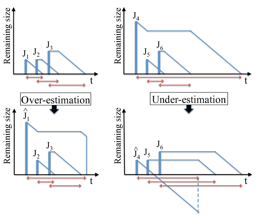
Figure 1: Examples of scheduling without (top) and with (bottom) errors.

In Fig. 1, we provide an illustrative example where a single job size is over- or under-estimated while the others are estimated correctly, focusing (because of its simplicity) on SRPTE; sojourn times are represented by the horizontal arrows. The left column of Fig. 1 illustrates the effect of over-estimation. In the top, we show how the scheduler behaves without errors, while in the bottom we show what happens when the size of job $J_{1}$ is over-estimated. The graphs shows the remaining (estimated) processing time of the jobs over time, assuming a normalized service rate of 1. Without errors, $J_{2}$ does not preempt $J_{1}$, and $J_{3}$ does not preempt $J_{2}$. Instead, when the size of $J_{1}$ is over-estimated, both $J_{2}$ and $J_{3}$ preempt $J_{1}$. Therefore, the only penalized job (i.e., experiencing higher sojourn time) is the over-estimated one. Jobs with smaller sizes are always able to preempt an over-estimated job, therefore the basic property of SRPT (favoring small jobs) is not significantly compromised.

The right column of Fig. 1 illustrates the effect of under-estimation. With no estimation errors (top), a large job, $J_{4}$, is preempted by small ones ($J_{5}$ and $J_{6}$). If the size of the large job is under-estimated (bottom), its estimated remaining processing time eventually reaches zero: we call late a job with zero or negative estimated remaining processing time. A late job cannot be preempted by newly arrived jobs, since their size estimation will always be larger than zero. In practice, since preemption is inhibited, the under-estimated job monopolizes the system until its completion, impacting negatively all waiting jobs.

This phenomenon is particularly harmful with heavily skewed job sizes, if estimation errors are proportional to size: if there are few very large jobs and many small ones, a single late large job can significantly delay several small ones, which will need to wait for the late job to complete for an amount of time which is disproportionate to their size before having an opportunity of being served.

Even if the impact of under-estimation seems straightforward to understand, surprisingly no work in the literature has ever discussed it. To the best of our knowledge, we are the first to identify this problem, which significantly influences scheduling policies dealing with inaccurate job size.

In FSPE, the phenomena we observe are analogous: job size over-estimation delays only the over-estimated job; under-estimation can result in jobs terminating in the virtual PS queue before than in the real system; this is impossible in absence of errors due to the dominance result introduced in Section 4.1. We therefore define late jobs in FSPE as those whose execution is completed in the virtual system but not yet in the real one and we notice that, analogously to SRPTE, also in FSPE late jobs can never be preempted by new ones, and they block the system until they are all completed.

5 Our Solution

Now that we have identified the issue with existing size-based scheduling policies, we propose a strategy to avoid it. It is possible to envision strategies that update job size estimations as work progresses in an effort to reduce errors; such solutions, however, increase the complexity both in designing systems and in analyzing them. In fact, the effectiveness of such a solution would depend non-trivially on the way size estimation errors evolve as jobs progress: this is inextricably tied to the way estimators are implemented and to the application use case. We propose, instead, a solution that requires no additional job size estimation, based on the intuition that late jobs should not prevent executing other ones. This goal is achievable with simple modifications to preemptive size-based scheduling disciplines such as SRPT and FSP; the key property is that the scheduler takes corrective actions when one or more jobs are late, guaranteeing that newly arrived small jobs will execute soon even when very large late jobs are running.

We conclude this section by showing our proposal, PSBS; it implements this idea while being efficient ($O(\log n)$ complexity) and allowing the usage of different weights to differentiate jobs. Our experimental results show that PSBS achieves almost optimal mean sojourn times for a large variety of workloads, suggesting that more complex solutions involving re-estimations are unlikely to be very beneficial in many practical cases.

5.1 Using PS and LAS for Late Jobs

From our analysis of Section 4.2, we understand that current size-based schedulers behave problematically when one or more jobs become late. Fortunately, it is possible to understand if jobs are late from the internal state of the scheduler: in SRPT, a job is late if its remaining estimated size is less than or equal to zero; in FSP, a job is late if it is completed in the virtual time but not in the real time.

As outlined above, approaches that involve job size re-estimation are difficult to design and evaluate, especially from the point of view of this work, where we do not make any assumption on the job size estimators; our approach, therefore, requires only one size estimation per job.

The key idea of our proposal is that late jobs should not monopolize the system resources. The solution is to modify the scheduler such that it provides service to a set of jobs, which we call eligible jobs, rather than a single job at a time. In particular, we consider the following jobs as eligible when at least one job is late: for our amended version of SRPTE, all the late jobs, plus the non-late job with the highest-priority; for our amended version of FSPE, only the late jobs.

The two cases differ because, in SRPTE, jobs only become late while they are being served since remaining processing time decreases only for them; therefore, non-late jobs need a chance to be served. We serve only one non-late job to minimize unnecessary deviations from SRPTE. In FSPE, conversely, jobs become late depending on the simulated behavior of the virtual time, independently from which jobs are served in the real time.

We take into account two choices for scheduling eligible jobs: PS and LAS (see Section 2.1). PS divides resources evenly between all jobs, while LAS divides resources evenly between the job(s) that received the least amount of service until the current time.

The alternatives proposed so far lead to four scheduling policies that we evaluate experimentally in Section 7:

1. SRPTE+PS. Behaving as SRPTE as long as no jobs are late, switching to PS between all late jobs and the highest-priority non-late job;

2. SRPTE+LAS. As above, but using LAS instead of PS;

3. FSPE+PS. Behaving as FSPE as long as no jobs are late, switching to PS between all late jobs;

4. FSPE+LAS. As above, but using LAS instead of PS.

We point out that, in the absence of errors or just of size underestimations, jobs are guaranteed to be never late; this means that in such cases these scheduling policies will be equivalent to SRPT(E) and FSP(E), respectively. For a more precise description, we point the interested reader to their implementation in our simulator.

5.2 PSBS

In Section 7.1 we show how the scheduling protocols we propose outperform, in most cases, both existing size-based scheduling policies and size-oblivious ones such as PS and LAS. Betweeen the scheduling protocols just introduced, we point out that FSPE+PS is the only one that guarantees to avoid starvation: every job will eventually complete in the virtual time, and therefore will be scheduled in a PS fashion. Conversely, both SRPTE and LAS can starve large jobs if smaller ones are continuously submitted. Due to this property and to the good performance we observe in the experiments of Section 7.2, we consider FSPE+PS a desirable policy. It has, however, a few shortcomings: first, it does not handle weights to differentiate job priorities; second, its implementation is inefficient, requiring $O(n)$ computation where $n$ is the number of jobs running in the emulated system. Here, we propose PSBS, a generalization of FSPE+PS which solves these problems, both allowing different job weights and having an efficient $O(\log n)$ implementation.

5.2.1 Job Weights

Neither FSP nor PS support job differentiation through job weights. In particular, FSP schedules jobs based on their completion time in a virtual time that simulates an environment using PS, which treats all running jobs equally.

To differentiate jobs in PSBS, we use Discriminatory Processor Sharing (DPS) [26] in the place of PS, both in the virtual time and in the scheduling for late jobs. DPS is a generalization of PS whereby each job is given a weight, and resources are shared between processes proportionally to their weight. By assigning a different weight to jobs, we can therefore prioritize important jobs. When all weights are the same, DPS is equivalent to PS; when each job has the same weight PSBS is equivalent to FSPE+PS.

Our handling of weights follows classic algorithms like Weighted Fair Queuing (WFQ) and Weighted Round Robin (WRR), accelerating aging (i.e., the decrease of virtual size) proportionally to weight, so that jobs with higher weight are scheduled earlier. Our result from Section 3 guarantees that PSBS dominates DPS if job sizes are known exactly, while at the same time being an online scheduler, implemented without any knowledge of jobs released in the future.

5.2.2 Implementation

FSP emulates a virtual system running a processor sharing (PS) discipline and keeps track of its job completion order; FSP then schedules one job at a time following that order. Whenever a new job arrives, FSP needs to update the remaining size of each job in the emulated system to compute the new virtual finish times and the corresponding job completion order. Existing implementations of FSP [2, 27] have $O(n)$ complexity due to the job virtual remaining size update at each arrival.

In our implementation, we reduce the complexity of the update procedure. Before showing the details of the algorithm, we introduce an example to help understand our solution. Consider three jobs ($J_{1}$, $J_{2}$ and $J_{3}$) with sizes $s_{1}=10$, $s_{2}=5$ and $s_{3}=2$ respectively, weights $w_{1}=w_{2}=w_{3}=1$, which arrive at times $t=0$, $t=3$ and $t=5$ respectively. Fig. 2 shows the evolution of the virtual emulated system, i.e., how the remaining virtual size decreases in the virtual time. For instance, when job $J_{3}$ arrives, since it will complete in the virtual time before jobs $J_{1}$ and $J_{2}$, it will be executed immediately in the real system (job $J_{2}$ will be preempted). To compute the completion time, it is possible to calculate the exact virtual remaining size of the jobs currently in the system.

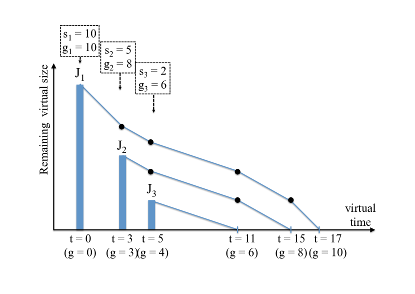
Figure 2: Example of virtual time $t$ and virtual lag $g$, used for sorting jobs.

We instead introduce a new variable, which we call virtual lag $g$. The key idea is that we store, for each job $i$, a job virtual lag $g_{i}$ so that $i$ completes in the virtual time when the virtual lag $g=g_{i}$. We fulfill this property by updating $g$ at a rate that depends on the number of jobs in the system: for each time unit in the virtual time, $g$ increases by $1/w_{v}$, where $w_{v}$ is the sum of the weights $w_{i}$ of each job $i$ running in the virtual emulated system.

Given a job $i$ with weight $w_{i}$ and size $s_{i}$ that arrives at the system when the virtual lag $g$ has a value $g=x$, the job virtual lag is given by $g_{i}=x+s_{i}/w_{i}$. The job virtual lag $g_{i}$ is computed just once, when the job arrives, and it does not need to be updated when other jobs arrive. In fact, only the global virtual lag $g$ needs to be updated according to the number of jobs in the system. Fig. 2 shows the job virtual lag computed when each jobs arrives (value of $g_{i}$ below $s_{i}$) and the value of the global virtual lag $g$ (below the virtual time $t$). Indeed, each job $i$ completes when $g=g_{i}$, but the only variable we update at each job arrival is $g$, leaving untouched the values $g_{i}$ of the job virtual lags. For instance, when job $J_{3}$ arrives, the virtual lag $g$ has value 4, therefore the job virtual lag will be $g_{3}=4+2$ (since the size and the weights of job $J_{3}$ are $s_{3}=2$ and $w_{3}=1$). It takes 6 time units (in the virtual time) to complete job $J_{3}$, which corresponds to 2 time units in the virtual lag.

It is simple to show that, given any positive value for $s_{i}$ and $w_{i}$, the order at which jobs complete in the virtual time and in the virtual lag is exactly the same. Therefore, at each job arrival, it is sufficient to update the global virtual lag $g$, compute the job virtual lag $g_{i}$ and store the object in a priority queue, where the order is kept according to the values of $g_{i}$. The overall complexity is dominated by the maintenance of the priority queue, which is $O(\log n)$, since it is not necessary to update the virtual remaining size of all jobs in the system to compute the completion order.

The implementation of our solution, shown in Algorithm 1, follows the nomenclature used in the original description of FSP [2, Section 4.4]. We remark that, in the absence of errors and when all job weights are the same, PSBS is equivalent to FSP: therefore, our implementation of PSBS is also the first $O(\log n)$ implementation of FSP.

”””Set up the scheduler state.
$\mathcal{O}$ and $\mathcal{E}$ contain $(i,g_{i},w_{i})$ tuples: $i$ is the job id, $g_{i}$ is the value of $g$ at which the job completes in the virtual time and $w_{i}$ is the weight. They are sorted by $g_{i}$. ”””

def Init:

      

      $g\leftarrow 0$ # virtual lag (see text)

      

      $t\leftarrow 0$ # virtual time

      

      # virtual time queue

       $\mathcal{O}\leftarrow$ empty binary min-heap

      

      # “early” jobs completed in real time

       $\mathcal{E}\leftarrow$ empty binary min-heap

      

      # mapping from job ids of late jobs to their weight

       $\mathcal{L}\leftarrow$ empty hashtable

      

      $w_{\mathcal{L}}\leftarrow 0$ # $\sum w_{i}$ for each late job $i$

      

      $w_{v}\leftarrow 0$ # $\sum w_{i}\forall i$ running in virtual time

      

def NextVirtualCompletionTime:

       if $\mathcal{O}$ and/or $\mathcal{E}$ are not empty:

             $\hat{g}\leftarrow\min\{\text{first $g_{i}$ in $\mathcal{O}$},\text{first $g_{i}$ in $\mathcal{E}$\}}$

             return $t+w_{v}(\hat{g}-g)$

      

      else:  return $\emptyset$

      

def UpdateVirtualTime($\hat{t}$):

       if $w_{v}>0$: $g\leftarrow g+(\hat{t}-t)/w_{v}$

       $t\leftarrow\hat{t}$

def VirtualJobCompletion($\hat{t}$):

       UpdateVirtualTime($\hat{t}$)

       if $\text{first $g_{i}$ in $\mathcal{O}$}\leq g$:

             $(i,\_,w_{i})\leftarrow\text{pop($\mathcal{O}$)}$

             $\mathcal{L}[i]\leftarrow w_{i}$

             $w_{\mathcal{L}}\leftarrow w_{\mathcal{L}}+w_{i}$

      

      else: # the virtual job that completes is in $\mathcal{E}$

             $(\_,\_,w_{i})\leftarrow\text{pop($\mathcal{E}$)}$

      

       $w_{v}\leftarrow w_{v}-w_{i}$

def RealJobCompletion($i$):

       if $\mathcal{L}$ is not empty: # we were scheduling late jobs

             $w_{i}\leftarrow pop(\mathcal{L}[i])$

             $w_{\mathcal{L}}\leftarrow w_{\mathcal{L}}-w_{i}$

            

      

      else: # we were scheduling the first job in $\mathcal{O}$

             push pop($\mathcal{O}$) into $\mathcal{E}$

      

      

def JobArrival($\hat{t},i,s_{i},w_{i}$):

       UpdateVirtualTime($\hat{t}$)

       push $(i,g+s_{i}/w_{i},w_{i})$ into $\mathcal{O}$

       $w_{v}\leftarrow w_{v}+w_{i}$

      

def ProcessJob:

       if $\mathcal{L}$ is not empty: return $\left\{(i,w_{i}/w_{\mathcal{L}}):(i,w_{i})\in\mathcal{L}\right\}$

      elif $\mathcal{O}$ is not empty: return $\{(\text{first job id of $\mathcal{O}$},1)\}$

      else:  return $\emptyset$

      

Algorithm 1 PSBS.

Computation is triggered by three events: if a job $i$ of weight $w_{i}$ and estimated size $s_{i}$ arrives at time $\hat{t}$, JobArrival($\hat{t},i,s_{i},w_{i}$) is called; when a job $i$ completes, RealJobCompletion($i$) is called; finally, when a job completes in virtual time at time $\hat{t}$, VirtualJobCompletion($\hat{t}$) is called (NextVirtualCompletionTime is used to discover when to call VirtualJobCompletion). After each event, ProcessJob is called to determine the new set of scheduled jobs: its output is a set of $(j,s)$ pairs where $j$ is the job identifier and $s$ is the fraction of system resources allocated to it.

As auxiliary data structures, we keep two priority queues, $\mathcal{O}$ and $\mathcal{E}$. $\mathcal{O}$ stores jobs that are running both in the real time and in the virtual time, while $\mathcal{E}$ stores “early” jobs that are still running in the virtual time but are completed in the real time. For each job $i$, we store in $\mathcal{O}$ or $\mathcal{E}$ an immutable tuple $(i,g_{i},w_{i})$ containing respectively the job id, the virtual lag $g_{i}$ and the weight. We use binary min-heaps to represent $\mathcal{O}$ and $\mathcal{E}$, using the $g_{i}$ values as ordering key: binary heaps are efficient data structures offering worst-case $O(\log n)$ “push” and “pop” operations, $O(1)$ lookup of the first value and eassentially optimal memory efficiency, by virtue of being an implicit data structure requiring no pointers [28]. In addition, the push operation has of $O(1)$ complexity on average [29]. The state of the scheduler is completed by a mapping $\mathcal{L}$ from the identifiers of late jobs to their weight, a counter $t$ representing the virtual time, and two variables $w_{v}$ and $w_{\mathcal{L}}$ representing the sum of weights for jobs that are respectively active in the virtual time and late. Some additional bookkeeping, not included here for simplicity, would be needed to handle jobs that complete even when they are not scheduled (e.g., because of error conditions or after being killed): we refer the interested reader to the implementation in our simulator. Additional details can be found in the supplemental material.

Complexity Analysis

We consider here average complexity due to the worst-case $O(n)$ complexity of hashtable operations. It is trivial to see that NextVirtualCompletionTime and UpdateVirtualTime have $O(1)$ complexity. Since inserting elements in hashtables has $O(1)$ average complexity, the cost of VirtualJobCompletion is dominated by the pop operations on $\mathcal{O}$ and $\mathcal{E}$: both of them are bound by $O(\log n)$, where $n$ is the number of jobs in the system. Removing an element from a hashtable has $O(1)$ average cost, so the cost of RealJobCompletion is dominated by the pop on $\mathcal{O}$, which has again $O(\log n)$ complexity. JobArrival has $O(1)$ average complexity (remember that pushing elements on a binary heap is $O(1)$ on average).

The ProcessJob procedure, when $\mathcal{L}$ is not empty, has $O(|\mathcal{L}|)$ complexity because the output itself has size $\mathcal{L}$. This is however very unlikely to be a limitation in practical cases, since real-world implementations of schedulers allocate resources one by one in discrete slots: schedulers such as PS or DPS are abstractions of mechanisms such as round-robin or max-min fair schedulers, which can be implemented efficiently; a real-world implementation of PSBS would adopt similar strategy to mimick the DPS-like resource sharing when $\mathcal{L}$ is not empty. We also note that, when there are no job size estimation errors and PSBS is used to implement FSP, $\mathcal{L}$ is guaranteed to always be empty and therefore ProcessJob will have $O(1)$ complexity.

As we have seen, with the exclusion of ProcessJob as discussed above, all the procedures of the scheduler have at most $O(\log n)$ computational complexity. Coupled $O(\log n)$ operations having low constant factors because they are implemented on binary heaps, which are very efficient data structures, we believe that these performance guarantees are sufficient for a very large set of practical situations: for example, CFS – the current Linux scheduler – has $O(\log n)$ complexity since it uses a tree structure [31].

6 Evaluation Methodology

Understanding size-based scheduling when there are estimation errors is not a simple task; analytical studies have been performed only with strong assumptions such as bounded error [9]. Moreover, to the best of our knowledge, the only analytical result known for FSP (without estimation errors) is its dominance over PS, making analytical comparisons between SRPTE-based and FSPE-based scheduling policies even more difficult.

For these reasons, we evaluate our proposals through simulation. The simulative approach is extremely flexible, allowing to take into account several parameters – distribution of the arrival times, of the job sizes, of the errors. Previous simulative studies (e.g., [8]) have focused on a subset of these parameters, and in some cases they have used real traces. In our work, we developed a tool that is able to both reproduce real traces and generate synthetic ones. Moreover, thanks to the efficiency of the implementation, we were able to run an extensive evaluation campaign, exploring a large parameter space. For these reasons, we are able to provide a broad view of the applicability of size-based scheduling policies, and show the benefits and the robustness of our solution with respect to the existing ones.

6.1 Scheduling Policies Under Evaluation

In this work, we take into account different scheduling policies, both size-based and size-oblivious. For the size-based disciplines, we consider SRPT as a reference for its optimality with respect to the MST. When introducing the errors, we evaluate SRPTE, FSPE and our proposals described in Section 5.

As size-oblivious policies, we have implemented the First In, First Out (FIFO) and Processor Sharing (PS) disciplines, along with DPS, the generalization of PS with weights [6]. These policies are the default disciplines used in many scheduling systems – e.g., the default scheduler in Hadoop [32] implements a FIFO policy, while Hadoop’s FAIR scheduler is inspired by PS; the Apache web server delegates scheduling to the Linux kernel, which in turn implements a PS-like strategy [16]. Since PS scheduling divides evenly the resources among running jobs, it is generally considered as a reference for its fairness (see the next section on the performance metrics). Finally, we consider also the Least Attained Service (LAS) [3] policy. LAS scheduling is a preemptive policy that gives service to the job that has received the least service, sharing it equally in a PS mode in case of ties. LAS scheduling has been designed considering the case of heavy-tailed job size distributions, where a large percentage of the total work performed in the system is due to few very large jobs, since it gives higher priority to small jobs than what PS would do.

6.2 Performance Metrics

We evaluate scheduling policies according to two main aspects: mean sojourn time (MST) and fairness. Sojourn time is the time that passes between the moment a job is submitted and when it completes; such a metric is widely used in the scheduling literature. The definition of fairness is more elusive: in his survey on the topic, [33] affirms that “fairness is an amorphous concept that is nearly impossible to define in a universal way”. When the job size distribution is skewed, it is intuitively unfair to expect similar sojourn times between very small jobs and much larger ones; a common approach is to consider slowdown, i.e. the ratio between a job’s sojourn time and its size, according to the intuition that the waiting time for a job should be somewhat proportional to its size. In this work we focus on the per-job slowdown, to check that as few jobs as possible experience “unfair” high slowdown values; moreover, in accordance with Wierman’s definition [34], we also evaluate conditional slowdown, which evaluates the expected slowdown given a job size, verifying whether jobs of a particular size experience an “unfair” high expected slowdown value.

6.3 Parameter Settings

Parameter	Explanation	Default
sigma	$\sigma$ in the log-normal error distribution	0.5
shape	shape for Weibull job size distribution	0.25
timeshape	shape for Weibull inter-arrival time	1
njobs	number of jobs in a workload	10,000
load	system load	0.9

TABLE I: Simulation parameters.

We empirically evaluate scheduling policies in a wide spectrum of cases. Table I synthetizes the input parameters of our simulator; they are discussed in the following.

Job Size Distribution

Job sizes are generated according to a Weibull distribution, which allows us to evaluate both heavy-tailed and light-tailed job size distributions. The shape parameter allows to interpolate between heavy-tailed distributions (shape $<1$), the exponential distribution (shape$=1$), the Raleigh distribution ($\text{shape}=2$) and light-tailed distributions centered around the ‘1’ value ($\text{shape}>2$). We set the scale parameter of the distribution to ensure that its mean is 1.

Since scheduling problems have been generally analyzed on heavy-tailed workloads with job sizes using distributions such as Pareto, we consider a default heavy-tailed case of $\text{shape}=0.25$. In our experiments, we vary the shape parameter between a very skewed distribution with $\text{shape}=0.125$ and a light-tailed distribution with $\text{shape}=4$.

Size Error Distribution

We consider log-normally distributed errors. A job having size $s$ will be estimated as $\hat{s}=sX$, where $X$ is a random variable with distribution

$$\operatorname{Log-\mathcal{N}}(0,\sigma^{2}).$$ (1)

This choice satisfies two properties: first, since error is multiplicative, the absolute error $\hat{s}-s$ is proportional to the job size $s$; second, under-estimation and over-estimation are equally likely, and for any $\sigma$ and any factor $k>1$ the (non-zero) probability of under-estimating $\hat{s}\leq\frac{s}{k}$ is the same of over-estimating $\hat{s}\geq ks$. This choice also is substanciated by empirical results: in our implementation of the HFSP scheduler for Hadoop [15], we found that the empirical error distribution was indeed fitting a log-normal distribution.

The sigma parameter controls $\sigma$ in Equation 1, with a default – used if no other information is given – of 0.5; with this value, the median factor $k$ reflecting relative error is 1.40. In our experiments, we let sigma vary between 0.125 (median $k$ is 1.088) and 4 (median $k$ is 14.85).

It is possible to compute the correlation between the estimated and real size as $\sigma$ varies. In particular, when sigma is equal to 0.5, 1.0, 2.0 and 4.0, the correlation coefficient is equal to 0.9, 0.6, 0.15 and 0.05 respectively.

The mean of this distribution is always larger than 1, and, as sigma grows, the system is biased towards overestimating the aggregate size of several jobs, limiting the underestimation problems that our proposals are designed to solve. Even in this setting, the results in Section 7 show that the improvements we obtain are still significant.

Job Arrival Time Distribution

For the job inter-arrival time distribution, we use again a Weibull distribution for its flexibility to model heavy-tailed, memoryless and light-tailed distributions. We set the default of its shape parameter (timeshape) to 1, corresponding to “standard” exponentially distributed arrivals. Also here, timeshape varies between 0.125 (very bursty arrivals separated by long intervals) and 4 (regular arrivals).

Other Parameters

The load parameter is the mean arrival rate divided by the mean service rate. As a default, we use 0.9 like [8]; in our experiments we let it vary between 0.5 and 0.999. The number of jobs (njobs) in each simulation round is 10,000. For each experiment, we perform at least 30 repetitions, and we compute the confidence interval for a confidence level of 95%. For very heavy-tailed job size distributions (shape $\leq 0.25$), results are very variable and therefore, to obtain stable averages, we performed hundreds and/or thousands of experiment runs, at least until the confidence levels have reached the 5% of the estimated values.

7 Experimental Results

We now proceed to an extensive report of our experimental findings. We first provide a high-level view showing that our proposals outperform PS, excepting only extreme cases of both error and job skew (Section 7.1); we then proceed to a more in-depth comparison of our proposals, to validate our choice of using FSPE+PS as a base for PSBS (Section 7.2). We then evaluate the performance of PSBS against existing schedulers, while varying the two parameters that most influence scheduler performance: shape (Section 7.3) and sigma (Section 7.4). We proceed to show that PSBS handles jobs fairly (Section 7.5) and that job weights are handled correctly (Section 7.6); we conclude our analysis on synthetic workloads by showing that our results hold even while varying settings over the parameter space (Section 7.7). We conclude our analysis by comparing PSBS to existing schedulers on real workloads extracted from Hadoop logs and an HTTP cache (Section 7.8).

For the results shown in the following, parameters whose values are not explicitly stated take the default values in Table I. For readability, we do not show the confidence intervals: for all the points, in fact, we have performed a number of runs sufficiently high to obtain a confidence interval smaller than 5% of the estimated value. Where not otherwise stated, all the $w_{i}$ parameters representing the weight of each job $i$ have always been set to 1.

7.1 Mean Sojourn Time Against PS

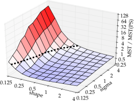
(a) SRPTE.

(b) SRPTE+PS.

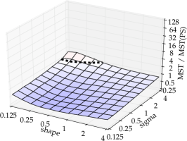
(c) SRPTE+LAS.

(d) FSPE.

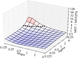
(e) FSPE+PS.

(f) FSPE+LAS.

Figure 3: Mean sojourn time against PS: the dashed line is the boundary where MST is equivalent to that of PS. We recall that a low shape value is associated to high job size skew, while high sigma entails imprecise job size estimates.

We begin our analysis by comparing the size-based scheduling policies, using PS as a baseline because PS and its variants are the most widely used set of scheduling policies in real systems. In Fig. 3 we plot the value of the MST obtained using SRPTE, FSPE and the four alternatives we propose in Section 5.1, normalizing it against the MST of PS. We vary the sigma and shape parameters influencing respectively job size distribution and error rate; we will see that these two parameters are the ones that influence performance the most. Values lower than one (below the dashed line in the plot) represent regions where size-based schedulers perform better than PS.

In accordance to intuition and to what is known from the literature, we observe that the performance of size-based scheduling policies depends on the accuracy of job size estimation: as sigma grows, performance suffers. In addition, from Figures 3a and 3d, we observe a new phenomenon: job size distribution impacts performance even more than size estimation error. On the one hand, we notice that large areas of the plots ($\textrm{shape}>0.5$) are almost insensitive to estimation errors; on the other hand, we see that MST becomes very large as job size skew grows ($\textrm{shape}<0.25$). We attribute this latter phenomenon to the fact that, as we highlight in Section 4, late jobs whose estimated remaining (virtual) size reaches zero are never preempted. If a large job is under-estimated and becomes late with respect to its estimation, small jobs will have to wait for it to finish in order to be served.

As we see in Figures 3b, 3c, 3e and 3f, our proposals outperform PS in a large class of heavy-tailed workloads where SRPTE and FSPE suffer. The net result is that the size-based policies we propose are outperformed by PS only in extreme cases where both the job size distribution is extremely skewed and job size estimation is very imprecise.

It may appear surprising that, when job size skew is not extreme, size-based scheduling can outperform PS even when size estimation is very imprecise: even a small correlation between job size and its estimation can direct the scheduler towards choices that are beneficial on aggregate. In fact, as we see more in detail in the following (Section 7.3), sub-optimal scheduling choices become less penalized as the job size skew diminishes.

7.2 Comparing Our Proposals

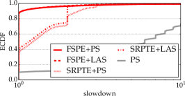
(a) $\text{shape}=0.25$.

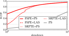
(b) $\text{shape}=1$.

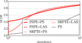
(c) $\text{shape}=4$.

Figure 4: Distribution of per-job slowdown. The two FSPE-based policies perform best, with negligible differences between them.

How do the schedulers we proposed in Section 5.1 compare? In Fig. 4 we examine the empirical cumulative distribution function (ECDF) of the slowdown for all jobs we simulate while varying the shape parameter (sigma maintains its default value of 0.5); we plot the results for PS as a reference and observe that the staircase-like pattern observable in Fig. 4a is a clustering around integer values obtained if a small job gets submitted while $n$ larger ones are running.

We observe that, in general, our proposals pay off: for all values of shape considered, the slowdown distribution of our proposals is well lower than the one of PS. We also observe a difference between the schedulers based on SRPTE and those based on FSPE: a noticeably larger number of jobs experience an optimal slowdown of 1 when using a scheduler based on FSPE. This is because, when using FSPE-based scheduling policies, the number of jobs that are eligible for PS- or LAS-based scheduling is higher: when late jobs exist, only they are eligible to be scheduled, unlike what happens in SRPTE-based policies; as a consequence, several small jobs suffer in SRPTE-based policies because they are preempted too aggressively: as soon as they become late, even if they are the only late job in the system. This confirms the soundness of the design policy we adopted in Section 5.1: minimizing the number of eligible jobs for PS- or LAS-based scheduling. Fig. 4 shows that even allowing to schedule a single non-late job can hurt performance.

Since the number of late jobs is generally small, differences in scheduling between FSPE+PS and FSPE+LAS are rare. This is confirmed by noticing that the lines for the two schedulers in Fig. 4 are essentially analogous; we conclude that FSPE+PS and FSPE+LAS have essentially analogous performance. This fact and the property that FSPE+PS avoids starvation, as noted in Section 5.2, motivated us to develop PSBS as a generalization of FSPE+PS.

7.3 Impact of Shape

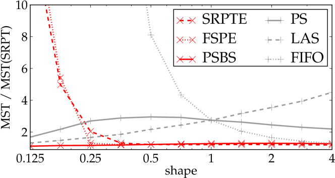
Figure 5: Impact of shape. PSBS behaves close to optimally in all cases.

After validating the choice of PSBS as a generalization of FSPE+PS, we now examine how it performs when compared to the optimal MST that SRPT obtains. In the following Figures, we show the ratio between the MST obtained with the scheduling policies we implemented and the optimal one of SRPT, while fixing sigma to its default value of 0.5.

From Fig. 5, we see that the shape parameter is fundamental for evaluating scheduler performance. We notice that PSBS has almost optimal performance for all shape values considered, while SRPTE and FSPE perform poorly for highly skewed workloads. Regarding non size-based policies, PS is outperformed by LAS for heavy-tailed workloads (shape $<1$) and by FIFO for light-tailed ones having $\text{shape}>1$; PS provides a reasonable trade-off when the job size distribution is unknown. When the job size distribution is exponential (shape $=1$), non size-based scheduling policies perform analogously; this is a result which has been proven analytically (see e.g. the work by [35] and the references therein). It is interesting to consider FIFO: in it, jobs are scheduled in series, and job priority is not correlated with size: indeed, the MST of FIFO is equivalent to the one of a random scheduler executing jobs in series [36]. FIFO can be therefore seen as the limit case for a size-based scheduler such as FSPE or SRPTE when estimations carry no information at all about job sizes; the fact that errors become less critical as skew diminishes can be therefore explained with the similar patterns observed for FIFO.

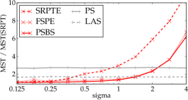
(a) $\text{shape}=0.25$

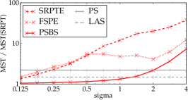
(b) $\text{shape}=0.177$

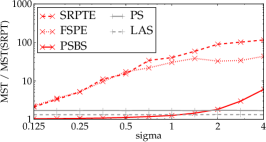
(c) $\text{shape}=0.125$

Figure 6: Impact of error on heavy-tailed workloads, sorted by growing skew.

7.4 Impact of Sigma

The shape of the job size distribution is fundamental in determining the behavior of scheduling algorithms, and heavy-tailed job size distributions are those in which the behavior of size-based scheduling differs noticeably. Because of this, and since heavy-tailed workloads are central in the literature on scheduling, we focus on those.

In Fig. 6, we show the impact of the sigma parameter representing error for three heavily skewed workloads. In all three plots, the values for FIFO fall outside of the plot. These plots demonstrate that PSBS is robust with respect to errors in all the three cases we consider, while SRPTE and FSPE suffer as the skew between job sizes grows. In all three cases, PSBS performs better than PS as long as sigma is lower than 2: this corresponds to lax bounds on size estimation quality, requiring a correlation coefficient between job size and its estimate of 0.15 or more.

In all three plots, PSBS performs better than SRPTE; the difference between PSBS and FSPE, instead, is discernible only for $\textrm{shape}<0.25$. We explain this difference by noting that, when several jobs are in the queue, size reduction in the virtual queue of FSPE is slow: hence, less jobs become late and therefore non preemptable. As the distribution becomes more heavy-tailed, more jobs become late in FSPE and differences between FSPE and PSBS become significant, reaching differences of even around one order of magnitude.

In particular in Fig. 6b, there are areas ($0.5<\text{sigma}<2$) in which increasing errors decreases (slightly) the MST of FSPE. This counterintuitive phenomenon is explained by the characteristics of the error distribution: the mean of the log-normal distribution grows as sigma grows, therefore the aggregate amount of work for a set of several jobs is more likely to be over-estimated; this reduces the likelihood that several jobs at once become late and therefore non-preemptable. In other words, FSPE works better with estimation means that tend to over-estimate job size; however, it is always better to use PSBS, which provides a more reliable and performant solution to the same problem.

In additional experiments – not included due to space limitations – we observed similar results with other error distributions; in cases where errors tend towards underestimations, we find that the improvements that PSBS gives over FSPE and SRPTE are even more important.

7.5 Fairness

We now consider fairness, intending – as discussed in Section 6.2 – that jobs’ running time should be proportional to their size, and therefore slowdowns should not be large.

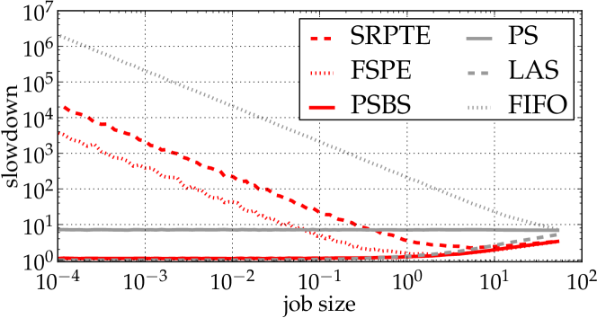
Figure 7: Mean conditional slowdown. PSBS outperforms PS, the scheduler often taken as a reference for fairness.

Conditional Slowdown

To better understand the reason for the unfairness of FIFO, SRPTE and FSPE, in Fig. 7 we evaluate mean conditional slowdown, showing average slowdown (job sojourn time divided by job size) against job size, using our default simulation parameters. The figure has been obtained by sorting jobs by size and binning them into 100 job classes having similar size and containing the same number of jobs; points plotted are obtained by averaging job size and slowdown in each of the 100 classes.

The lines of FIFO, SRPTE and FSPE are almost parallel for smaller jobs because, below a certain size, job sojourn time is essentially independent from job size: indeed, it depends on the total size of older (for FIFO) or late (for SRPTE and FSPE) jobs at submission time.

We confirm experimentally that the expected slowdown in PS is constant, irrespectively of job size [34]; PSBS and LAS, on the other hand, have close to optimal slowdown for small jobs. PSBS has a better MST because it performs better for larger jobs, which are more penalized in LAS.

(a)

(b)

Figure 8: Per-job slowdown: full CDF (top) and zoom on the 10% more critical cases (bottom).

Per-Job Slowdown

Our results testify that, for PSBS and similarly to LAS, slowdown values are homogeneous across classes of job sizes: neither small nor big jobs are penalized when using PSBS. This is a desirable result, but the reported results are still averages: to ensure that sojourn time is commensurate to size for all jobs, we need to investigate the per-job slowdown distribution.

In Fig. 8, we plot the CDF of per-job slowdown for our default parameters. By serving efficiently smaller jobs, size-based scheduling techniques and LAS manage to obtain an optimal slowdown of 1 for most jobs. However, some jobs experience very high slowdown: those with slowdown larger than 100 are around 1% for FSPE and around 8% for SRPTE. PS, LAS, and PSBS perform well in terms of fairness, with no jobs experiencing slowdown higher than 100 in our experiment runs. While PS is generally considered the reference for a “fair” scheduler, it obtains slightly better slowdown than LAS and PSBS only for the most extreme cases, while being outperformed for all other jobs.

7.6 Job Weights

(a) $\text{shape}=0.25$

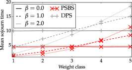
(b) $\text{shape}=1$

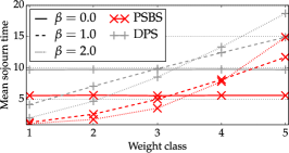
(c) $\text{shape}=4$

Figure 9: Using weights to differentiate jobs: PSBS outperforms DPS.

We now consider how PSBS handles job weights. We consider workloads generated with all the default values shown in Table I. Since we are not aware of representative workloads where job priorities and job sizes are known together, we resort to a simple uniform distribution. We randomly assign jobs to different weight classes numbered from 1 to 5 with uniform probability: a job $i$ in weight class $c_{i}$ has weight $w_{i}=1/c_{i}^{\beta}$, where $\beta\geq 0$ is a parameter that allows us to tune how much we want to skew scheduling towards favoring high-weight jobs. A $\beta=0$ value corresponds to uniform weights, $w_{i}=1$ for each job; as $\beta$ grows, job weights differentiate so that more and more resources are assigned to high-weight jobs.

In Fig. 9, we plot the mean sojourn time for jobs in each weight class. Jobs have a mean size of 1: therefore, the best MST obtainable would be 1, which corresponds to the bottom of the graph. We compare the results of PSBS with those obtained by generalized processor sharing (DPS) while using the same weights.

For workloads ranging between heavily skewed ($\text{shape}=0.25$) to close to uniform ($\text{shape}=4$), PSBS outperforms DPS. Obviously, $\beta=0$ leads to uniform MST between weight classes; raising the values of $\beta$ improves the performance of high-weight jobs to the detriment of low-weight ones. When $\beta=2$, the MST of jobs in class 1 is already very close to the optimal value of 1; we do not consider values of $\beta>2$ because it would impose performance losses to low-weight jobs without significant benefits to high-weight ones. It is interesting to point out that the trade-off due to the choice of $\beta$ is not uniform across values of shape: when the workload is close to uniform ($\text{shape}=4$), improvements in sojourn times for high-weight jobs are quantitatively similar to the losses paid by low-weight ones; this is because high-weight jobs are likely to preempt low-weight ones with similar sizes. Conversely, with heavily skewed workloads ($\text{shape}=0.25$) sojourn time improvements for high-weight jobs are smaller than losses for low-weight ones: this is because, in skewed workloads, large high-weight jobs are likely to preempt small low-weight ones: this results in small improvements in sojourn time for the high-weight jobs, counterbalanced by large losses for the low-weight ones.

7.7 Other Settings

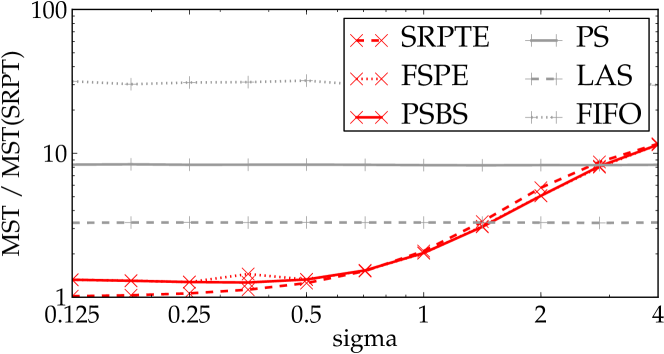
(a) $\alpha=2$

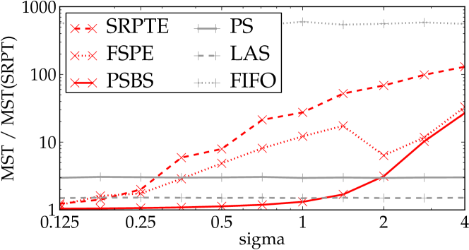
(b) $\alpha=1$

Figure 10: Pareto job size distributions, sorted by growing skew.

Until here, we focused on the sigma and shape parameters, because they are the ones that we found out to have the most influence on scheduler behavior. We now examine the impact of other settings that deviate from our defaults.

Pareto Job Size Distribution

In the literature, workloads are often generated using the Pareto distribution. To help comparing our results to the literature, in Fig. 10 we show results for job sizes having a Pareto distribution, using $x_{m}=0$ and $\alpha=\{1,2\}$. The results we observe for the Weibull distribution are still qualitatively valid for the Pareto distribution; the value of $\alpha=1$ is roughly comparable to a shape of 0.15 for the Weibull distribution, while $\alpha=2$ is comparable to a shape of around 0.5, where the three size-based disciplines we take into account still have similar performance.

Impact of Other Parameters

We have studied the impact of other parameters, such as the load, the timeshape and the njobs, and the results are consistent with the ones showed in the previous sections. The interested reader can find the details in the supplemental material.

7.8 Real Workloads

We now consider two real workloads to confirm that the phenomena we observed are not an artifact of the synthetic traces that we generated, and that they indeed apply in realistic cases. From the traces we obtain two data points per job: submission time and job size. In this way, we move away from the assumptions of the $GI/GI/1$ model, and we provide results that can account for more general cases where periodic patterns and correlation between job size and submission times are present.

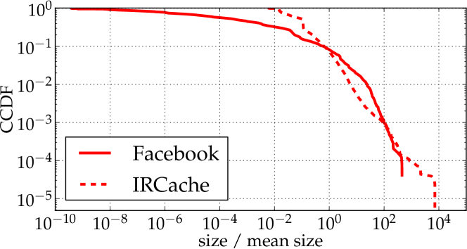
Figure 11: CCDF for the job size of real workloads.

Hadoop at Facebook

We consider a trace from a Facebook Hadoop cluster in 2010, covering one day of job submissions. The trace has been collected and analized by [37]; it is comprised of 24,443 jobs and it is available online. For the purposes of this work, we consider the job size as the number of bytes handled by each job (summing input, intermediate output and final output): the mean size is 76.1 GiB, and the largest job processes 85.2 TiB. To understand the shape of the tail for the job size distribution, in Fig. 11 we plot the complementary CDF (CCDF) of job sizes (normalized against the mean); the distribution is heavy-tailed and the largest jobs are around 3 orders of magnitude larger than the average size. For homogeneity with the previous results, we set the processing speed of the simulated system (in bytes per second) in order to obtain a load (total size of the submitted jobs divided by total length of the submission schedule) of 0.9.

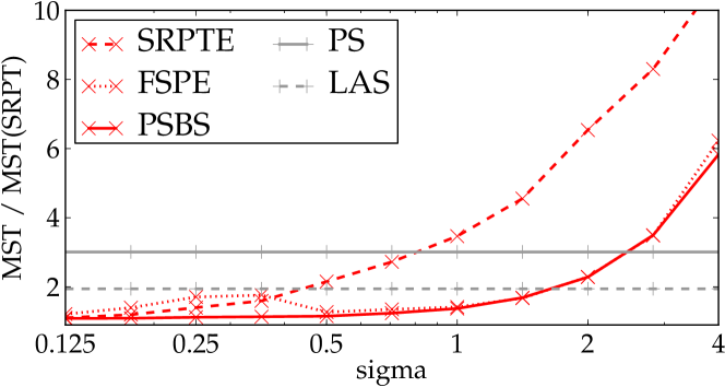
Figure 12: MST of the Facebook workload.

In Fig. 12, we show MST, normalized against optimal MST, while varying the error rate. These results are very similar to those in Fig. 6: once again, FSPE and PSBS perform well even when job size estimation errors are far from negligible. These results show that this case is well represented by our synthetic workloads, when shape is around 0.25.

We performed more experiments on these traces; extensive results are available in a technical report [38].

Web Cache

IRCache is a research project for web caching; traces from the caches are freely available. We performed our experiments on a one-day trace of a server from 2007 totaling 206,914 requests; the mean request size in the traces is 14.6KiB, while the maximum request size is 174 MiB. In Fig. 11 we show the CCDF of job size; as compared to the Facebook trace analyzed previously, the workload is more heavily tailed: the biggest requests are four orders of magnitude larger than the mean. As before, we set the simulated system processing speed in bytes per second to obtain a load of 0.9.

Figure 13: MST of the IRCache workload.

In Fig. 13 we plot MST as the sigma parameter controlling error varies. Since the job size distribution is heavy-tailed, sojourn times are more influenced by job size estimation errors (notice the logarithmic scale on the $y$ axis), confirming the results we have from Fig. 3. The performance of FSPE does not worsen monotonically as error grows, but rather becomes better for $0.5<\text{sigma}<1$; this is a phenomenon that we also observe – albeit to a lesser extent – for synthetic workloads in Fig. 6b and for the Facebook workload in Fig. 12. The explanation provided in Section 7.4 applies: since the mean of the log-normal distribution grows as sigma grows, the aggregate amount of work for a given set of jobs is likely to be over-estimated in total, reducing the likelihood that several jobs at once become late and therefore non-preemptable. Also here, we still remark that PSBS consistently outperforms FSPE.

8 Conclusion

This work shows that size-based scheduling is an applicable and performant solution in a wide variety of situations where job size is known approximately. Limitations shown by previous work are, in a large part, solved by the approach we took for PSBS; analogous measures can be taken in other preemtpive size-based disciplines.

PSBS is a generalization of FSP, and we have proven analytically that, in the absence of errors, it dominates DPS; to the best of our knowledge, PSBS is also the first $O(\log n)$ implementation of FSP.

With PSBS, system designers do not need to worry about the problems created by job size under-estimations. PSBS also solves a fairness problem: while FSPE and SRPTE penalize small jobs and results in slowdown values which are not proportionate to their size, PSBS has an optimal slowdown equal to 1 for most small jobs.

We maintain that, thanks to its efficient implementation, solid performance in case of estimation errors, and support for job weights, PSBS is a practical size-based policy that can guide the design of schedulers in real, complex systems. We argue that it is worthy to try size-based scheduling, even if inaccurate estimates can be produced to estimate job sizes: our proposal, PSBS, is reasonably easy to implement and provides close to optimal response times and good fairness in all but the most extreme of cases.

We released our simulator as free software; it can be reused for: (i) reproducing our experimental results; (ii) prototyping new scheduling algorithms; (iii) predicting system behavior in particular cases, by replaying traces.

Matteo Dell’Amico is a researcher at Symantec Research Labs; his research revolves on the topic of distributed computing. He received his M.S. (2004) and Ph.D. (2008) in Computer Science from the University of Genoa (Italy); during his Ph.D. he also worked at University College London. Between 2008 and 2014 he was a researcher at EURECOM. His research interests include data-intensive scalable computing, peer-to-peer systems, recommender systems, social networks, and computer security.

Damiano Carra received his Laurea in Telecommunication Engineering from Politecnico di Milano, and his Ph.D. in Computer Science from University of Trento. He is currently an Assistant Professor in the Computer Science Department at University of Verona. His research interests include modeling and performance evaluation of peer-to-peer networks and distributed systems.

Pietro Michiardi received his M.S. in Computer Science from EURECOM and his M.S. in Electrical Engineering from Politecnico di Torino. Pietro received his Ph.D. in Computer Science from Telecom ParisTech (former ENST, Paris). Today, Pietro is a Professor of Computer Science at EURECOM. Pietro currently leads the Distributed System Group, which blends theory and system research focusing on large-scale distributed systems (including data processing and data storage), and scalable algorithm design to mine massive amounts of data. Additional research interests are on system, algorithmic, and performance evaluation aspects of computer networks and distributed systems.

Appendix A Supplemental material

A.1 Simulator Implementation Details

Our simulator is available under the Apache V2 license. It has been conceived with ease of prototyping in mind: for example, our implementation of FSPE as described in Section 4 requires 53 lines of code. Workloads can be both replayed from real traces and generated synthetically.

The simulator has been written with a focus on computational efficiency. It is implemented using an event-based paradigm, and we used efficient data structures based on B-trees. As a result of these choices, a “default” workload of 10,000 jobs is simulated in around half a second, while using a single core in our 2011 laptop with an Intel T7700 CPU. We use IEEE 754 double-precision floating point values to represent time and job sizes.

A.2 Additional experiments

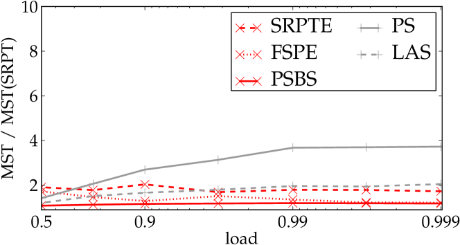
(a) Varying load.

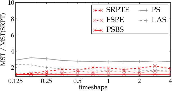
(b) Varying timeshape.

Figure 14: Impact of load and timeshape.

In Fig. 14, we show the impact of load and timeshape, keeping sigma and shape at their default values. Fig. 14a shows that performance of size-based scheduling protocols is not heavily impacted by load, as the ratio between the MST obtained and the optimal one remains roughly constant (note that the graph shows a ratio, and not the absolute values which increase as the load increases); conversely, size-oblivious schedulers such as PS and LAS deviate more from optimal as the load grows. Fig. 14b shows the impact of changing the timeshape parameter: with low values of timeshape, job submissions are bursty and separated by long pauses; with high values job submissions are more evenly spaced. We note that size-based scheduling policies respond very well to bursty submissions where several jobs are submitted at once: in this case, adopting a size-based policy that focuses all the system resources on the smallest jobs pays best; as the intervals between jobs become more regular, SRPTE and FSPE become slightly less performant; PSBS remains close to optimal.

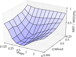
(a) Varying load.

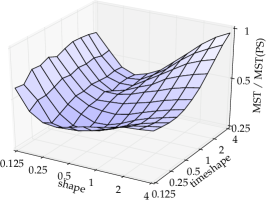
(b) Varying timeshape.

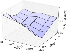
(c) Varying njobs.

Figure 15: PSBS against PS.

With Fig. 15, we show that the results of Fig. 14 generalize to other parameter choices: by letting shape vary together with load, timeshape and njobs, we notice that PSBS always performs better than PS. The V-shaped pattern, where the difference in performance between the two schedulers is larger for “central” values of the shape parameter is essentially caused by PS performing closer to optimal for extreme values of the shape parameter, as we can see in Fig. 5.

References

- Schrage and Miller [1966] L. E. Schrage and L. W. Miller, “The queue M/G/1 with the shortest remaining processing time discipline,” Operations Research, vol. 14, no. 4, pp. 670–684, 1966.