Spin dynamics of Mn impurities and their bound acceptors in GaAs

Abstract

We present results of tight-binding spin-dynamics simulations of individual and pairs of substitutional Mn impurities in GaAs. Our approach is based on the mixed quantum-classical scheme for spin dynamics, with coupled equations of motions for the quantum subsystem, representing the host, and the localized spins of magnetic dopants, which are treated classically. In the case of a single Mn impurity, we calculate explicitly the time evolution of the Mn spin and the spins of nearest-neighbors As atoms, where the acceptor (hole) state introduced by the Mn dopant resides. We relate the characteristic frequencies in the dynamical spectra to the two dominant energy scales of the system, namely the spin-orbit interaction strength and the value of the $p$-$d$ exchange coupling between the impurity spin and the host carriers. For a pair of Mn impurities, we find signatures of the indirect (carrier-mediated) exchange interaction in the time evolution of the impurity spins. Finally, we examine temporal correlations between the two Mn spins and their dependence on the exchange coupling and spin-orbit interaction strength, as well as on the initial spin-configuration and separation between the impurities. Our results provide insight into the dynamic interaction between localized magnetic impurities in a nano-scaled magnetic-semiconductor sample, in the extremely-dilute (solotronics) regime.

I INTRODUCTION:

Recently, remarkable progress has been achieved in describing the electronic and magnetic properties of individual dopants in semiconductors, both experimentallyYakunin et al. (2004); Kitchen et al. (2006); Bocquel et al. (2013) and theoretically Tang and Flatté (2004); Strandberg et al. (2009); Mahani et al. (2014), offering exciting prospects in future electronic devices. In view of novel potential applications, which involve communication between individual magnetic dopants, mediated by electronic degrees of freedom of the host, the focus of this research field has been shifting towards fundamental understanding and control of spin dynamics of these atomic-scale magnetic centers. Importantly, the development of advanced spectroscopic techniques has opened up the possibility to probe the dynamics of single spin impurities experimentally Khajetoorians et al. (2013). Some specific examples include inelastic tunneling spectroscopy of atomic-scale magnetic structures Hirjibehedin et al. (2006), optical manipulation of spin-centers in semiconductors Fuchs et al. (2009), magnetic resonance imaging D. Rugar and Chui (2004); Grinolds et al. (2011, 2014) and time-resolved scanning tunneling spectroscopy Loth et al. (2010) on single spins. These advances pose new challenges for theory, calling for a fully microscopic time-dependent description of spin dynamics of individual spin impurities in the solid-state environment.
The most suitable approach to study the time evolution of spin systems, which is applicable at ultrashort time ($\lesssim 100$ ps) and length ($\lesssim 1$ nm) scales and does not rely on phenomenological parameters, is ab initio spin dynamics (SD). A natural framework for this approach is provided by the extension of density functional theory (DFT) to time domain and noncollinear spins (time-dependent spin DFT, or TD-SDFT), with several practical schemes developed to date Antropov et al. (1996, 1995); Kurth et al. (2005); F hnle et al. (2005); Skubic et al. (2008); Stamenova and Sanvito (2013). However, due to computational demands, the system sizes that can be treated with this approach are limited to only a handful of atoms Stamenova and Sanvito (2013). In practice, numerical implementations typically rely on approximations. A well-known example is the adiabatic ab initio SD model by Antropov et al. Antropov et al. (1996, 1995), which is based on a Born-Oppenheimer(BO)-type approximation for spin degrees of freedom in materials with localized magnetic moments. Because of the difference in the characteristic energy scales for itinerant and localized spins, this model treats the directions of the local magnetic moments as slow classical variables, while averaging over the fast electronic degrees of freedom. Such separation leads to an equation of motion for the classical moments interacting with an effective field.
Antropov’s SD model provides the theoretical framework for large-scale implementations of atomistic spin dynamics, such as the one by Skubic et al. Skubic et al. (2008). In the latter approach, the equation of motion for the localized magnetic moments is augmented by a phenomenological damping term (in analogy with Landau-Lifshitz-Gilbert equation) and by a stochastic (Langeven) term, which accounts for the effect of finite temperature. This scheme was used to investigate magnetic ordering and correlations in clusters of Mn-doped GaAs at finite temperature Hellsvik et al. (2008). We also mention that, apart from standard atomistic spin-dynamics approaches, beyond mean-field dynamical models have been developed Morandi et al. (2009), which specifically address ultrafast photoenhanced magnetization dynamics in dilute magnetic semiconductors (DMSs), in particular (Ga, Mn)As Wang et al. (2007).
In this work we employ the mixed quantum-classical SD model Stamenova and Sanvito (2010), which is similar in spirit albeit different in some important aspects from Antropov’s adiabatic SD, to study the dynamics of individual and pairs of Mn impurities in GaAs. Although our model assumes a partition into a quantum subsystem, representing the electrons of the host (GaAs), and a classical subsystem, representing the localized magnetic moments of the dopants (Mn), the interaction between the two subsystems is treated at the level of the Ehrenfest approximation Horsfield et al. (2004), as opposed to the BO approximation. This results in a system of coupled equations of motion, with the two subsystems evolving simultaneously and experiencing each other as time-varying classical fields. As already known from its application to electron-ion dynamics  Horsfield et al. (2004), such scheme is able to capture non-adiabatic effects on the fast electronic time scale (fs), which are inaccessible by the BO approximation. Recently, Ehrenfest SD has been used to study the effects of electrostatic gating in atomistic spin conductors Pertsova et al. (2011).
In order to describe the underlying electronic structure of the semiconductor host, we use a microscopic tight-binding (TB) model for GaAs with parameters fitted to DFT calculations. This gives our approach a computational edge compared to purely ab initio SD, which relies on the Kohn-Sham Hamiltonian Antropov et al. (1996). The spins of Mn dopants are introduced in the Hamiltonian as classical vectors exchange coupled to the instantaneous spin-densities of the nearest-neighbors As atoms, in the spirit of the $p$-$d$ exchange interaction. In the static regime, this TB model has already proved successful in describing experimentally observed properties of single Mn dopants and their associated acceptor states in GaAs Strandberg et al. (2009); Mahani et al. (2014).
Here we explore the solotronics limit of DMSs Koenraad and Flatté (2011) in the time domain by probing explicitly the time evolution of individual substitutional Mn dopants in a finite nanometer-size cluster of GaAs. From the time-dependent spin-trajectories of single-impurity spins, we identify the characteristic energy scales of the dynamics, associated with intrinsic interactions present in the system, namely the $p$-$d$ exchange interaction and the spin-orbit interaction (SOI). Furthermore, we study the time evolution of two Mn-impurity spins upon an arbitrary perturbation of one of the spins. The SD simulations allow us to address explicitly the time-dependent (dynamic) indirect exchange interaction between the spins, which is expected to differ from its static counterpart Fransson (2010), and is relevant for nanostructures with magnetic impurities Costa et al. (2008). We map out the temporal correlations between the two localized spins, expressed in terms of a classical spin-spin correlation function, as a function of the SOI, $p$-$d$ exchange interaction, spatial separation, and the initial orientations of the spins ( e.g. ferromagnetic, antiferromagnetic and noncollinear configurations). The variations in strength and time scale of the correlations, inferred from behavior of the spin-spin correlation function for different system parameters, can be used as an indicative measure of dephasing of individual impurity spins due to their interaction with the host and other impurities.
The paper is organized as follows. In Section II we describe the details of our theoretical approach. In Section III we discuss the results of numerical simulations. Section III.1 is concerned with the effect of SOI and exchange coupling strength on the time evolution of a single Mn spin. In Section III.2 we study the dynamical interplay between two spatially-separated Mn impurities, coupled indirectly by carrier-mediated exchange interaction. Finally we draw some conclusions.

II THEORETICAL MODEL

II.1 Tight-binding Hamiltonian

We begin to lay out the computational framework of our SD simulations by first defining the respective Hamiltonians of the two subsystems. The time-dependent Hamiltonian of the GaAs host (quantum subsystem), incorporating a number of substitutional Mn atoms on Ga sites, takes the following form

$$\hat{H}_{el}(t) =\sum_{ii^{\prime},\mu\mu^{\prime},\sigma}t_{\mu\mu^{\prime}}^{ii^{\prime}}\hat{c}_{i\mu\sigma}^{{\dagger}}\hat{c}_{i^{\prime}\mu^{\prime}\sigma}+J_{pd}\sum_{m}\sum_{n[m]}\vec{S}_{m}(t)\cdot\hat{\vec{s}}_{n}$$

$$+\sum_{i,\mu\mu^{\prime},\sigma\sigma^{\prime}}\lambda_{i}\langle\mu,\sigma|\hat{\vec{L}}\cdot\hat{\vec{s}}|\mu^{\prime},\sigma^{\prime}\rangle\hat{c}_{i\mu\sigma}^{{\dagger}}\hat{c}_{i\mu^{\prime}\sigma^{\prime}}$$

$$+\frac{e^{2}}{4\pi\varepsilon_{0}\varepsilon_{r}}\sum_{m}\sum_{i\mu\sigma}\frac{\hat{c}_{i\mu\sigma}^{{\dagger}}\hat{c}_{i\mu\sigma}}{|\vec{r}_{i}\mathbf{-}\vec{R}_{m}|}+V_{\rm Corr},$$ (1)

where $i$($i^{\prime}$) is the atomic index that runs over all atoms, $m$ runs over the Mn atoms, and $n[m]$ over the nearest-neighbors (NN) of $m$-the Mn atom; $\mu$($\mu^{\prime}$) labels atomic orbitals ($s$, $p_{x,y,z}$) and $\sigma$($\sigma^{\prime}$) is the spin index; $t_{\mu\mu^{\prime}}^{ii^{\prime}}$ are the Slater-Koster parameters Chadi (1977) and $\hat{c}_{i\mu\sigma}^{{\dagger}}$($\hat{c}_{i\mu\sigma}$) is the creation(annihilation) operator. Below, we briefly discuss the meaning of all the terms on the right-hand side of Eq. (1). For a more detailed description the reader is referred to Ref. Strandberg et al., 2009.

The first term in Eq. (1) is the nearest-neighbors $sp^{3}$ Slater-Koster Hamiltonian Slater and Koster (1954); Papaconstantopoulos and Mehl (2003) that reproduces the band structure of bulk GaAs Chadi (1977). The second term represents the antiferromagnetic ($p$-$d$) exchange coupling between the Mn spin $\vec{S}_{m}$ (originating from the $d$-levels of the dopant and treated here as a classical vector) and the nearest-neighbor As $p$-spins, $\hat{\vec{s}}_{n}=1/2\sum_{\pi\sigma{\sigma^{\prime}}}\hat{c}_{n\pi\sigma}^{\dagger}\vec{\tau}_{\sigma{\sigma^{\prime}}}\hat{c}_{n\pi{\sigma^{\prime}}}$, where $\vec{\tau}_{\sigma{\sigma^{\prime}}}$ are elements of the Pauli matrices $\vec{\tau}=\{\tau^{\alpha}\}$ ($\alpha=x,y,z$) and the orbital index $\pi$ runs over three As $p$-orbitals. We chose the value of the exchange coupling $J_{pd}=1.5$ eV, which has been been reported in the literature Timm and MacDonald (2005); Ohno (1998). Note that $\vec{S}_{m}$ is a unit vector and the magnitude of the Mn magnetic moment (5/2) is absorbed by the exchange coupling parameter.

The third term represents the one-body intra-atomic (on-site) SOI, where $\hat{\vec{L}}$ is the orbital moment operator, $\hat{\vec{s}}$ is the spin operator, $|\mu,\sigma\rangle$ are spin- and orbital-resolved atomic orbitals, corresponding to atom $i$, and $\lambda_{i}$ are the renormalized spin-orbit-splitting parameters Chadi (1977) ($\lambda_{\mathrm{As}}=0.14$ eV, $\lambda_{\mathrm{Ga}}=0.058$ eV and $\lambda_{\mathrm{Mn}}=0.058/2$ eV).

The fourth term represents the long-range repulsive Coulomb potential, dielectrically screened by the host material, with $\epsilon_{r}=12$ for bulk GaAs Teichmann et al. (2008); Lee and Gupta (2011). $\vec{r}_{i}$ and $\vec{R}_{m}$ denote the position of atom $i$ and the $m$-th classical spin, respectively. The last term, $V_{\rm Corr}$, is the central-cell correction to the impurity potential. This consists of the on-site part $V_{\mathrm{\rm on}}$, acting on the Mn ion, and the off-site part $V_{\mathrm{\rm off}}$, which affects the NN As atoms and is important for capturing the physics of the $p$-$d$ hybridization, in addition to the exchange interaction ($J_{pd}$). The value $V_{\mathrm{\rm on}}=1.0$ eV is inferred from the Mn ionization energy, and we set $V_{\mathrm{\rm off}}=2.4$ eV to reproduce the experimentally observed position of the Mn-induced acceptor level in bulk GaAs Schairer and Schmidt (1974); Lee and Anderson (1964); Chapman and Hutchinson (1967); Linnarsson et al. (1997).

We note that the time-dependence in the electronic Hamiltonian is carried by the Mn classical spins, $\vec{S}_{m}(t)$. At time $t$, the classical Hamiltonian of the $m$-th Mn spin is written as

$$H_{S}(t) =J_{pd}\sum_{n[m]}\langle\hat{\vec{s}}_{n}\rangle(t)\cdot\vec{S}_{m}(t).$$ (2)

This describes the exchange coupling between $\vec{S}_{m}$ and the total instantaneous spin-density of the NN As $p$-spins, defined as a sum of expectation values $\langle\hat{\vec{s}}_{n}\rangle(t)=\mathrm{Tr}\left[\hat{\rho}(t)\hat{\vec{s}}_{n}\right]$, where $\hat{\rho}(t)$ is the density matrix of the electronic subsystem at time $t$.

The dynamical properties of substitutional Mn atoms in a GaAs matrix are obtained by performing time-dependent SD simulations for a super-cell-type structure, consisting of a cubic cluster with $32$ atoms and periodic boundary conditions applied in three dimensions. The equations of motion which, together with the definitions of the quantum and classical Hamiltonians [Eqs. (1) and (2)], make up the core of the SD simulation, are described in the next section.

II.2 Equations of motion

The time evolution of the quantum subsystem is governed by the Liouville-von Neumann equation for the density matrix, while the localized spins, representing the Mn magnetic moments, evolve according to its classical analogue. Thus the system of coupled equations of motion reads

$$\left\{\begin{aligned} \dfrac{d\hat{\rho}(t)}{dt}&=\dfrac{i}{\hbar}\left[\hat{\rho}(t),\hat{H}_{el}(t)\right]\quad\\ \dfrac{d\vec{S}_{m}(t)}{dt}&=\left\{\vec{S}_{m}(t),H_{S}(t)\right\},\end{aligned}\right.$$ (3)

where $\left[\,,\,\right]$ denotes the commutator and $\left\{\,,\,\right\}$ the Poisson bracket. Using the classical analogue of the commutation relations for $\vec{S}_{m}$ Yang and Hirschfelder (1980), we can calculate explicitly the Poisson bracket and the classical equation of motion becomes

$$\dfrac{d\vec{S}_{m}(t)}{dt} =\dfrac{J_{pd}}{S}\sum_{n[m]}\left\langle\hat{\vec{s}}_{n}\right\rangle(t)\times\vec{S}_{m}(t)$$ (4)

where $S$ is the magnitude of $\vec{S}_{m}$.

As one can see from Eq. (3), the quantum and the classical subsystems evolve according to their respective equations of motion but are coupled through instantaneous exchange terms, which enter the time-dependent Hamiltonians $\hat{H}_{\rm el}(t)$ [Eq. 1] and $H_{S}(t)$ [Eq. 2]. Such coupled system represents the Ehrenfest approximation to spin dynamics Horsfield et al. (2004). This is in contrast to the BO approximation, in which the fast (quantum) degrees of freedom are integrated out. The equations of motion are integrated numerically using the fourth-order Runge-Kutta algorithm. The typical duration of the simulation is of the order of $10$ ps. We chose a time step $dt=0.001$ fs, which insures that the total energy is conserved within an error of $10^{-9}$ eV.

III RESULTS AND DISCUSSION

III.1 Single Mn impurity

We first consider a single Mn impurity replacing a Ga in the center of a 4-atom GaAs cluster. A smaller cluster size allows us to increase the simulation time up to $10$ ps, in order to understand the evolution of the spins and all the energy scales involved in the dynamics. In Section III.2 the size of the cluster will be increased to 32 atoms to study the SD in the presence of two Mn spins.

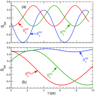
Figure 1: (Color online) Time evolution of the total spin of the system $\vec{S}^{\mathrm{tot}}$ for two choices of the perturbation, (a) $\theta=\phi=5^{\circ}$, and (b) $\theta=\phi=45^{\circ}$. Different components of the total spin are marked by arrows.

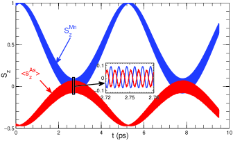
Figure 2: (Color online) Time evolution of the $z$-components of the spins of the Mn impurity ($S^{\mathrm{Mn}}_{z}$) and its NN As atoms ($\langle s^{\mathrm{As}}_{z}\rangle$). The inset shows the zoom-in into smaller time scale.

Before the start of the simulation (at $t$=$0$), the orientation of the classical Mn spin is fixed along the [001] direction. This corresponds to the $z$-axis, $\vec{S}_{m}(0)\parallel z$, or $\theta=\varphi=0$ in spherical coordinates, where $\phi$ is the azimuthal angle and $\theta$ is the polar angle. The calculations of magnetic anisotropy landscape for a Mn impurity in bulk GaAs, described with the classical-spin model used in this work, have shown that the [001] direction is the easy axis, while the plane perpendicular to it ($x$-$y$) is the hard plane Strandberg et al. (2009). For this equilibrium orientation, the electronic density matrix is constructed as $\hat{\rho}(0)=\sum_{\nu}f_{\nu}|\psi_{\nu}\rangle\langle\psi_{\nu}|$, where $\{\psi_{\nu}\}$ are the eigenfunctions of $\hat{H}_{el}(0)$ (see Eq. 1) and $f_{\nu}$ are Fermi-Dirac occupation numbers. The initial NN As spin-density, entering the classical Hamiltonian in Eq. (2), is calculated as $\langle\vec{s}^{\mathrm{As}}\rangle(0)=\sum_{n[m]}\langle\hat{\vec{s}}_{n}(0)\rangle=\sum_{n[m]}\mathrm{Tr}\left[\hat{\rho}(0)\hat{\vec{s}}_{n}\right]$.
In order to initiate the SD, the Mn spin is tilted from its preferential axis by angles $\theta$ and $\varphi$. This procedure represents an arbitrary external perturbation, applied locally to the Mn magnetic moment, e.g. a laser pulse or an external magnetic field. As an output of the simulation we obtain the time-dependent Cartesian components of the Mn spin, which will be denoted as $\vec{S}^{\mathrm{Mn}}$ throughout this section, as well as the time-dependent expectation value of the spin at any given atom $i$ of the cluster, $\langle\vec{s}_{i}\rangle$. We will focus in particular on the total spin $\langle\vec{s}^{\mathrm{As}}\rangle$ of the NN As atoms, where the Mn-induced spin-polarized acceptor state resides, and the total spin of the system defined as $\vec{S}^{\mathrm{tot}}=\vec{S}^{\mathrm{Mn}}+\sum_{i}\langle\vec{s}_{i}\rangle$, where $i$ runs over all Ga and As atoms.
Figure 1 shows the time evolution of the three components of the total spin $\vec{S}^{\mathrm{tot}}$ for two different choices of the perturbation, namely $\theta=\varphi=5^{\circ}$ and $\theta=\varphi=45^{\circ}$. The first choice corresponds to a weak perturbation since at the start of the simulation the Mn spin deviates only slightly from its preferential axis. We will use this type of perturbation in this section. Throughout the next section, III.2, we will use a slightly stronger perturbation, $\theta=\varphi=10^{\circ}$, unless specified otherwise.
As one can see from Fig. 1(a), all three components of $\vec{S}^{\mathrm{tot}}$ exhibit long-period ($\approx 5.5$ ps) oscillations, which appear by turning on the SOI. Note that without SOI the three components of the total spin are constants of motion and do not change during the time evolution. We conclude that in the case of a weak perturbation the dynamics of the total magnetic moments is mainly driven by the SOI. This is expected since the Mn spin remains in equilibrium with the spins of the NN As atoms. However, a strong perturbation ($\theta=\phi=45^{\circ}$) brings about the interplay between $\vec{S}^{\mathrm{Mn}}$ and $\langle\vec{s}^{\mathrm{As}}\rangle$, governed by the exchange coupling $J_{pd}$. This results in short-period ($\approx 500$ fs) oscillations, superimposed on the long-period and large-amplitude precession due to SOI [see Fig. 1(b)].
A similar effect, namely the appearance of pronounced oscillations due to $J_{pd}$, will be observed if we artificially scale up the exchange constant. Note also that the strong perturbation forces the $z$-component of the total spin to oscillate between two easy axes (parallel or anti-parallel to the $z$-axis), while in the case of the weak perturbation $\vec{S}^{\mathrm{tot}}$ remains above the $x$-$y$ plane ($S^{\mathrm{tot}}_{z}>0$).
The comparison between panels 1(a) and (b) also indicates that the resulting dynamics   and the oscillation frequency are sensitive to initial conditions, especially for strong perturbations beyond the linear-response regime.
Figure 2 shows the time evolution of the $z$-components of the Mn spin and the spin of the NN As atoms. Similarly to $S^{\mathrm{tot}}_{z}$ [Fig. 1(a)], the dynamics is governed by the long-period precession. However, the zoom-in into smaller times reveals fast oscillations due to $J_{pd}$. $S^{\mathrm{Mn}}_{z}$ and $\langle s^{\mathrm{As}}_{z}\rangle$ are oscillating in anti-phase, in accordance with the antiferromagnetic nature of the $p$-$d$ exchange coupling.
In order to understand how the characteristic energy scales of the system control its dynamics, we perform SD simulations with modified values of exchange and SOI parameters. As a references set of parameters, we consider the values of the spin-orbit splittings $\lambda_{i}$ and the exchange interaction $J_{pd}$ typically used in our TB model for (Ga,Mn)As. Next, we consider two cases: (i) the exchange interaction is unchanged and the SOI strength is $10\lambda_{i}$ and (ii) the SOI is unchanged and the exchange interaction is $4J_{pd}$. The time evolution of the Mn and NN As spins, calculated with the reference set and with the modified parameters, is shown in Figs. 3(a) and (b), respectively.

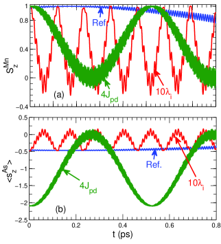
Figure 3: (Color online) Time evolution of the $z$-components of the Mn spin (a) and the spin of the NN As atoms (b) for three different choices of exchange and SOI parameters: (i) the reference case (see text for details), (ii) the case in which $\lambda_{\mathrm{i}}$ is increased by a factor of $10$ and (iii) the case in which $J_{pd}$ is increased by a factor of $4$. Only the first 800 fs of the total simulation time of $10$ ps are shown.

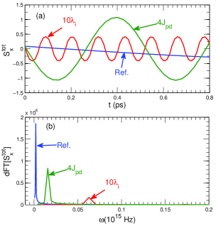
Figure 4: (Color online) (a) Time evolution of the $x$-component of the total spin of the system and (b) its discrete Fourier transform, for three different choices of exchange and SOI parameters. Notations are the same as in Fig. 3.

From the simulation with the reference set, we identify two main periods (frequencies), namely the long-period (low-frequency) oscillations and the short-period (high-frequency) oscillations. As mentioned before, these two characteristic periods are most likely associated with SOI and with exchange interaction, respectively, since $J_{pd}$ is several orders of magnitude larger than $\lambda_{i}$. This is further confirmed by the simulations with the modified parameters. Increasing the SOI strength, while keeping $J_{pd}$ unchanged, leads to a decrease of the long period. At the same time the period of rapid oscillations, superimposed on the dominant long-period precession, remains practically unchanged.
Increasing the exchange parameter by a factor of $4$ yields a significant decrease of the short period oscillations. However, there is also a noticeable change (decrease) in the long period oscillations. This is due to the fact that, in principle, one should not expect the two energy scales to affect the dynamics in a completely independent way. The complex dynamics of our combined quantum-classical system results from the interplay of the interactions (rather than simply from a superposition of harmonic motions with different frequencies). The change in $J_{pd}$ has the strongest effect on both short-period and long-period dynamics since it is the largest energy scale in the system.

The effect of the two energy scales can be also observed in the time evolution of the total spin. The time-dependent $x$-component of the total spin and its discrete Fourier transform (dFT) are shown in Fig. 4(a) and (b), respectively. For all three choices of parameters the long-period oscillations due to SOI are the most pronounced. The period of these oscillations is approximately $5.5$ ps for the reference set, which is equivalent to the frequency of $10^{12}Hz$. The latter can be associated with the position of the major peak in the corresponding dFT [see Fig. 1(b)]. Increasing the SOI strength leads to an increase of the characteristic period and to a shift of the characteristic frequency to the higher range. An increase of the exchange coupling parameter has a similar effect although the shift is smaller.

III.2 Two Mn impurities

In this section we focus on the dynamical interaction between two spatially separated Mn spins. We use a GaAs cluster illustrated in Fig. 5. The effects of the interaction parameters (exchange coupling and SOI), initial configuration of the spins and the separation between the impurity atoms on the dynamics will be investigated. Throughout this section the two classical spins are labeled as $\vec{S}^{1}$ and $\vec{S}^{2}$.

Figure 5: (Color online) A finite cluster of GaAs, consisting of $32$ atoms, with two Mn impurities. The separation between the impurities is $d\approx 0.8$ nm.

We first consider the situation when the two Mn spins are initially pointing along the $z$-direction. At the start of the simulation, one of the Mn spins is tilted by a small angle, $\theta=\varphi=10^{\circ}$, from its initial orientation. Figure 6 shows the time evolution of the $x$-components of both Mn spins and the spins of the corresponding NN As atoms for three different values of the exchange interaction (similar curves are obtained for other spin-components). The dynamics is almost identical for the two Mn spins, which is a signature of the ferromagnetic coupling between the two. Each of the localized spins is coupled antiferromagnetically to the spins of its NN As atoms, resulting in characteristic anti-phase oscillations.

The SD simulations reveal a short delay, or response time (of the order of $1$ fs for $J_{pd}=1.5$ eV), between the perturbation and the response of the second spin. The response time decreases with increasing the strength of the exchange interaction $J_{pd}$ between each of the individual Mn spins and the spins of the NN As atoms. This means that the spin perturbation, generated by the precession of the first (tilted) spin is transferred more efficiently to the second spin, when the exchange interaction between the Mn impurity spins and the host carriers is stronger. As a result, the effective dynamical interaction between the two impurity spins is enhanced. We can identify a characteristic time-interval $\tau_{d}$ (time delay) such that when the two curves, corresponding to the two Mn spins, are shifted by $\tau_{d}$, they appear to oscillate in a similar way ($\tau_{d}=10$ fs for $J_{pd}=1.5$ eV). This is essentially the time needed to establish the correlation between the two Mn spins. The value of $\tau_{d}$ decreases with $J_{pd}$. When the time delay is taken into account, the short period oscillations of the spins can be simply superimposed on each other, as shown in Figs. 7(a) and (b).

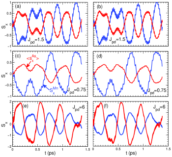
Figure 6: (Color online) The time evolution of the $x$-components of the two Mn spins (blue curves) and the spins of their respective NN As atoms (red curves) for (a,b) $J_{pd}=1.5$ eV, (c,d) $J_{pd}=0.75$ eV and (e,f) $J_{pd}=6$ eV. Left panels are for the first (tilted) Mn spin and right panels are for the second Mn.

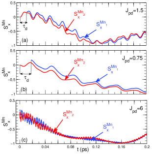
Figure 7: (Color online) Time evolution of the $x$-components of the two Mn spins during the first 200 fs from the start of the simulation, for (a) $J_{pd}=1.5$ eV, (b) $J_{pd}=0.75$ eV and (c) $J_{pd}=6$ eV. Notations are the same as in Fig. 6. Note that the blue curves (tilted spin) in panels (a) and (b) are shifted by the time delay $\tau_{\mathrm{d}}$ (see text for details) to show the similarity in the time evolution of the two spins at later times.

In order to understand how the electronic subsystem (GaAs host) mediates the propagation of spin disturbance between the localized spins, depending on the system parameters, we calculate the classical spin-spin correlation function Stamenova and Sanvito (2010)

$$C(S^{1}_{x},S^{2}_{x},\Delta{t}) =\frac{1}{N}\int{S^{1}_{x}(t)S^{2}_{x}(t+\Delta{t})dt}\;,$$ (5)

where $\Delta t$ is the time lag and $N$ is the normalization factor

$$N =\left\{\int{\left[S^{1}_{x}(t)\right]^{2}dt}\right\}^{\frac{1}{2}}\cdot\left\{\int{\left[S^{2}_{x}(t)\right]^{2}dt}\right\}^{\frac{1}{2}}.$$ (6)

Here we focus on the temporal correlations between the transverse ($x$) components of the spins, corresponding to deflections away from the easy axis. However, longitudinal components have also been considered and the resulting correlation functions show a similar behavior.

A few remarks are in order about the definition and the meaning of the classical cross-correlation function in Eqs. (5) and (6). In principle, for continuous functions of time, the integrals in the cross-correlation function are taken over the total simulation time $T$ in the limit $T\rightarrow\infty$, i.e. $\int\rightarrow\lim\limits_{T\rightarrow\infty}\int\limits_{0}^{T}$. For functions sampled on a finite time-interval $T$, the integrals are replaced by finite sums and the correlation function becomes Buck et al. (2002)

$$C(S^{1}_{x},S^{2}_{x},\Delta{t}) =\frac{1}{N}\sum_{i=0}^{N_{st}-\Delta{t}}{S^{1}_{x}(t_{i})\cdot S^{2}_{x}(t_{i}+\Delta{t})}\;,$$ (7)

where $t_{i}=i\cdot dt$, $\Delta t=j\cdot dt$ and $j$ runs from $1$ to $N_{st}$, with $N_{st}=T/dt$ being the total number of time steps. The normalization factor now reads

$$N =\left\{\sum_{i=0}^{N_{st}}{S^{1}_{x}(t_{i})\cdot S^{1}_{x}(t_{i})}\right\}^{\frac{1}{2}}\cdot\left\{\sum_{i=0}^{N_{st}}{S^{2}_{x}(t_{i})\cdot S^{2}_{x}(t_{i})}\right\}^{\frac{1}{2}}.$$ (8)

In this work we adopt the latter definition.

The cross-correlation function $C$, defined above, measures the similarity in the temporal profiles of two signals (in this case the two Mn spins) over the total simulation time, as a function of the time lag $\Delta{t}$ applied to one of them (this simply means that one of the signals is probed at a later time $t+\Delta{t}$ compared to the other one). The properties of the correlation function are described below.

The amplitude of $C$ at a given $\Delta t$ is a direct measure of the correlation between the two signals: if the correlation function has a node ($C=0$), the two signals are completely uncorrelated, while $C=1$ means that the signals are essentially identical; note that due to the normalization factor, $\mathrm{max}\left\{|C|\right\}\leq 1$. Let us first consider two sinusoidal signals, which have the same period but differ by a phase. The correlation function $C$ in this case is also a sinusoidal function with the same period. The value of $C$ at zero time lag depends on the phase difference between the two signals and varies in the interval $[-1,1]$. In the ideal case of an infinite integration interval, such correlation function would oscillate forever without decay, with an amplitude changing between $-1$ to $1$. If we now add a random contribution to the second signal, the amplitude of oscillations of the correlation function will decrease, since the coherence between the two signals is hindered.

However, for signals sampled on a finite time-interval, an additional issue affects the amplitude of the correlation function. Indeed, the integration interval, i.e. the number of terms in the finite sum in Eq. (7), becomes smaller as the time lag increases. Therefore, the amplitude of the correlation function decreases with the time lag and vanishes for $\Delta t$ equal to the total simulation time (even for two identical sinusoidal signals). This decay is linear as a function of the time lag in the above example and it is negligible when the maximum time lag is much smaller than the integration interval.

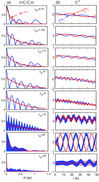
Figure 8: (Color online) (a) The absolute value of the correlation function $\left|C(S^{1}_{x},S^{2}_{x},\Delta{t})\right|$, plotted as a function of the time lag $\Delta t$, for different values of $J$. The fitting exponential functions $a\cdot e^{-\Delta{t}/\tau}$ are shown in red. (b) Time evolution of the $x$-component of the first (blue curve) and second spin (red curve).

Hence, we conclude that for realistic signals, two distinct factors affect the amplitude of the correlation function: (i) the coherence, or the phase difference between the two signals at a given time lag, which may result in an increase or a decrease of the amplitude and is physically meaningful, and (ii) the decay of the amplitude as a function of the time lag due to finite integration interval, which is inherent in the definition of the correlation function for sampled signals [see Eq. (7)]. In practice, it is problematic to separate the artificial decay due to finite integration intervals from the decay due to the gradual loss of coherence (dephasing) between the signals with increasing time lag. However, any increase or non-linear decay of $C$ can be associated with the level of coherence. It is also meaningful to compare the oscillating behavior and the decay of the correlation function for different system parameters, with respect to a reference parameter set. As shown below, the information extracted from the correlation function will be used mainly as a comparative measure of the temporal correlations between the two Mn spins.
Figure 8(a) shows the absolute value of $C(S^{1}_{x},S^{2}_{x},\Delta{t})$ as a function of the time lag $\Delta t$, for different values of the exchange coupling $J_{pd}$. The curves are fitted to an exponential function

$$f(\Delta t) =a\cdot e^{-\Delta{t}/\tau}.$$ (9)

where $a$ is a constant and $\tau$ is the characteristic decay time, with parameters listed in Table 1. The constant $a$ indicates the degree of correlation between the two spins while $\tau$ is the combined measure of the intrinsic decay due to limited integration interval and the fluctuations due to the phase difference between the two spins for increasing time lag. While the period of the oscillations and the constant $a$ are more robust, the value of $\tau$ depends on the integration interval $T$ (here $T=2$ ps) and it gradually goes to zero as the time lag becomes comparable to $T$. Although the value of $\tau$ for a given $J_{pd}$ does not necessarily indicate the decay due to dephasing of the two spins, comparing this value for different panels in Fig. 8(a) provides insight into how quickly the correlation dies out for different $J_{pd}$.

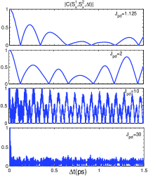
Figure 9: (Color online) (a) The absolute value of the correlation function $\left|C(S^{1}_{x},S^{2}_{x},\Delta{t})\right|$, plotted as a function of the time lag $\Delta t$, for different values of $J_{pd}$. Note that the integration scheme for the correlation function used here differs from the rest of the paper (see text for details).

Table 1: Parameters for the fitting functions in Fig. 8(a). The correlation function for different $J_{pd}$.

$J_{pd}$ (eV)	a	$\tau$ (fs)
0.75	1.0	155
1.125	0.66	389
1.5	0.69	328
2.0	0.6	508
6.0	0.69	586
10.0	0.34	718
20.0	0.6	200
30.0	0.61	15

To further clarify the issues related to the definition of the correlation function, we present in Fig. 9 the absolute value of $C(S^{1}_{x},S^{2}_{x},\Delta{t})$ calculated using a different integration scheme. Here the total simulation time is $T=4$ ps and the integration interval is $[0+\Delta t,T/2+\Delta t]$ ps, i.e. the sum in Eq. (7) runs from $i=j$ to $i=N_{st}/2+j$. Therefore, as the time lag increase, the integration interval remains constant ($T/2=2$ ps). The results obtained with this integration scheme clearly show that the decay of the correlation function seen in Fig. 8(a) is, indeed, partly caused by the dephasing between the two spins at larger time lags. Notably, the decay in the first two panels of Fig. 9, which is not caused by the decrease in the integration interval, is in agreement with the corresponding panels in Fig. 8(a). The slower decay for $J_{pd}=10$ eV and the very fast decay for $J_{pd}=30$ eV are also in agreement with Fig. 8(a) and with the values of the fitting parameters in Table 1. We should also mention that for all cases considered, the exponential fitting curve has better fitting statistics than a linear fit. This further confirms that $\tau$ captures part of the decay coming from the dephasing of the two spins. However, in the rest of the paper, we use the value of $\tau$ as a comparative rather than absolute measure of the dephasing.
We will now discuss in detail the behavior of the correlation function for different values of $J_{pd}$, shown in Fig. 8(a). The peak in the amplitude of the correlation function occurs at a very early time compared to the total simulation time. This confirms the observation that the transfer of the spin perturbation between the two spins, mediated by the host carriers, happens on a very fast time scale, e.g. $\sim 10$ fs (see Fig. 7). The degree of correlation at $\Delta t=0$, $a$, is maximum for $J_{pd}=0.75$ and nearly constant ($a\approx 0.6-0.7$) for other values (except a somewhat special intermediate case of $J_{pd}=10$ eV). In contrast, the decay time $\tau$ varies significantly with $J_{pd}$. It reaches its maximum for $J_{pd}\approx 10$ eV and decreases afterward. For exchange interactions in this range, the system is in a transient regime, before it undergoes a transition to a new dynamical state in which the Mn spins are effectively decoupled.

The long-period oscillations of the correlation function for $J_{pd}<10$ eV indicate that the frequency of precession of the tilted spin of precession of the tilted spin is not comparable to, i.e. it is much smaller than the characteristic electronic frequency or “electron ticking time”. The latter is the inverse of the time needed for the spin perturbation to travel forth and back between the two spins. For $J_{pd}\gtrsim 10$ eV these frequencies become comparable, and the correlation function oscillates very rapidly as a function of the time lag. It is also for a $J_{pd}$ around this value that the temporal correlations become long-ranged (the value $\tau$ is maximum in Table 1). This essentially means that the dynamical coupling between the localized spins is the strongest in this regime. Going over to yet larger values of $J_{pd}$, the carriers are too localized to transfer the spin perturbation efficiently, and therefore the spins become decoupled. This is also consistent with the short decay time of the correlation function $\tau\approx 15$ fs for $J_{pd}=30$ eV.

This behavior is consistent with time evolution of the transverse components of the spins [right panels of Fig. 8]. Except for a short time delay for small values of $J_{pd}$, the motion of the two spins is correlated for $J_{pd}\lesssim 10$ eV. However, for very large values of $J_{pd}$ the second spin completely looses the high-frequency component and even oscillates in anti-phase with the first spin, disrupting the ferromagnetic coupling between the two.
For a better understanding of the correlation between the two spins, we consider Mn atoms at different separations. The time-dependent trajectories of the two spins, when they are nearest neighbors (separation $d=0.4$ nm), reveal that the time delay for the second spin, observed in Fig. 7, is now shorter due to closer distance. More importantly the two spins are now behaving as they are strongly coupled. Figure 10(a) shows the correlation function and the exponential fitting curves for the case when the Mn atoms are nearest neighbors, for different values of the exchange coupling (the parameters of the fitting are listed in Table 2). As one can see, even for very large $J_{pd}=30$ eV, the spins are not completely decoupled: the decay time $\tau$ is roughly an order of magnitude larger than in the case of larger separation.
Comparing Tables 1 and 2 gives us some information about the dependence of the correlation between the spins on their separation. The characteristic decay time is consistently larger at smaller separation indicating that spins stay correlated longer. Note that the strength of correlation, given by parameter $a$, does not change dramatically for the values of $J_{pd}$ considered here and is close to the one found at larger separation ($a$ is maximum for $J_{pd}$ and is slightly smaller than average for extremely large $J_{pd}$).

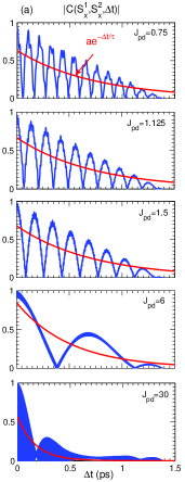
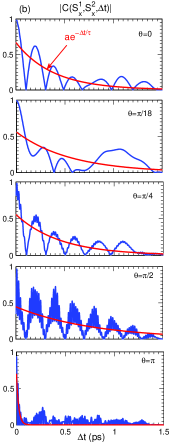
Figure 10: (Color online) (a) The absolute value of the correlation function $\left|C(S^{1}_{x},S^{2}_{x},\Delta{t})\right|$, plotted as a function of the time lag (blue curves), and the corresponding exponential fitting functions (red curves), for different values of $J_{pd}$. The Mn spins are nearest-neighbors. (b) The same correlation function for the case when the second spin is initiated at different angles ($\theta$ varies from $0$ to $\pi$ and $\phi=0$, $J_{pd}$ is fixed at the reference value).

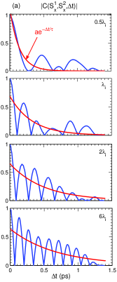
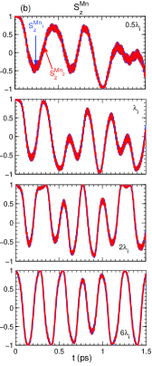
Figure 11: (Color online) (a) The absolute value of the correlation function $\left|C(S^{1}_{x},S^{2}_{x},\Delta{t})\right|$, plotted as a function of the time lag (blue curves), and the corresponding exponential fitting functions (red curves) for different values of SOI. (b) Time evolution of of the $z$-components of the two spins for the same values of SOI.

Table 2: Parameters for the fitting curves in Fig. 10 (a). Correlation function for different $J_{pd}$ when the Mn atoms are nearest neighbors.

$J_{pd}$ (eV)	a	$\tau$ (fs)
0.75	0.63	740
1.125	0.67	731
1.5	0.68	719
6.0	0.85	513
30.0	0.56	169

Table 3: Parameters for the fitting curves in Fig. 10(b). Correlation function for different initial configurations of Mn spins.

the direction of the second spin at $t=0$
$\phi=0$	a	$\tau$ (fs)
$\theta=0$	0.67	383
$\theta=\pi/18$	0.56	560
$\theta=\pi/4$	0.56	452
$\theta=\pi/2$	0.45	798
$\theta=\pi$	0.7	22.4

Table 4: Parameters for the fitting curves in Fig. 11(a). Correlation function for different SOI strength ($\lambda_{i}$). The $\lambda_{i}$ are the reference values of the spin-orbit interaction strength for the three different atoms in the system.

$\lambda_{i}$	a	$\tau$ (fs)
0.5$\lambda_{i}$	1.11	141.6
$\lambda_{i}$	0.69	328.2
2$\lambda_{i}$	0.65	502.3
6$\lambda_{i}$	0.64	682.5

It is instructive to analyze the dependence of the correlation function on the initial orientation of the two Mn spins, as it provides insight into which configuration is more favorable for long-range temporal correlations. Such analysis is presented in Fig. 10(b). At $t=0$ the first spin is pointing along $[001]$ direction while the second spin is tilted by an angle $\theta$ (we set $\varphi=0$). We consider a ferromagnetic (FM), $\theta=0$, antiferromagnetic (AFM), $\theta=\pi$, and non-collinear (NC), $0<\theta<\pi$, configurations. The parameters for the exponential fitting functions are listed in Table 3. The spins are most correlated for the FM configuration. In the NC case, the spins are still correlated and the characteristic decay time is even larger then in the FM case. However, the level of correlation is smaller, in particular for $\theta=\pi/2$. For the AFM configuration, the spins become completely decoupled, with the correlation function decaying rapidly within the first $\sim 20$ fs.
Finally, we probe the correlation function for different SOI [Fig. 11(a)]. The strength of SOI directly affects the magnetic anisotropy of the Mn magnetic moment, i.e. the magnetic anisotropy increases with increasing $\lambda_{i}$. Based on this, one might expect that for larger SOI the two Mn spins will not be able to cross the hard plane during their time evolution (the anisotropy barrier in the $x$-$y$ plane defined by $\theta=\pi/2$ and arbitrary $\varphi$). However, the analysis of the time-dependent longitudinal components of the two spins reveals the opposite. According to Fig. 11(b), $S_{z}^{1,2}(t)$ oscillate, switching between $[001]$ to $[00\bar{1}]$ directions, for all value of $\lambda_{i}$ considered. Therefore the anisotropy energy is not high enough to prevent the Mn spins from crossing the hard plane. However, as $\lambda_{i}$ increases, the Mn spins tend to spend less time around the hard plane and oscillate more rapidly between the two easy-axis directions.
Interestingly, the temporal correlations between the spins become stronger. As one can see from Table 4, which contains the parameters of the fitting functions, $\tau$ increases with $\lambda_{i}$ while $a$ saturates to a value of $0.6$ typical for our system. Similar to the case of increasing $J_{pd}$ (for $J_{pd}<10$ eV), the frequency of the long-period oscillations in the dynamics of the Mn spins increases and becomes comparable (although still smaller) to the electron ticking rate. This results in more rapidly oscillating correlation functions and larger decay times.

IV Conclusions

In this paper we studied the time evolution of substitutional Mn impurities in GaAs, using quantum-classical spin-dynamics simulations, based on the microscopic tight-binding model and the Ehrenfest approximation. We described the effect of spin-orbit and exchange interactions on the dynamical spectrum. A remarkable feature emerging from our simulations are long-period ($\sim 5.5$ ps) oscillations of the total magnetic moment due to the presence of the spin-orbit interaction.
Furthermore, we studied the spin dynamics in a system consisting of two separated Mn impurities. We calculated the classical spin-spin correlation functions as a measure of the effective dynamical coupling between the impurity spins. Our results demonstrate the dependence of this coupling on the properties of the electronic subsystem (GaAs), as well as on the spatial configuration of the impurity atoms and the initial orientation of their spins.
We find that increasing the exchange coupling facilitates the dynamical communication between the spins, mediated by the electronic degrees of freedom of the host. However, very strong exchange interaction tends to decouple the two spins as the host carriers become localized. For smaller spacial separation between the impurity atoms, the characteristic decay time of the correlation function increases significantly for all values of $J_{pd}$. When the spins are initialized in the same direction (or slightly tilted) they remain ferromagnetically coupled, with a characteristic in-phase oscillation pattern, over times of the order of few hundred femtoseconds. In contrast to this, when starting from an antiferromagnetic configuration, the decay time decrease to tens of femtoseconds. Increasing the spin-orbit interaction strength seems to have a similar effect as the exchange interaction (at least for small values of $J_{pd}$), i.e. the temporal correlations between the two spins become more long-ranged. We note, however, that the energy scale associated with the spin-orbit interaction is orders of magnitude smaller than that of the exchange interaction.
The role of the electronic subsystem of the host material, as well as the effects of inter- and intra-atomic interactions (exchange and spin-orbit interactions), on the dynamics of individual atomic-scale magnets are important questions that are becoming accessible experimentally. The present study contributes to fundamental understanding of spin dynamics in such devices, which is crucial for future applications in solotronics.