Optimization-based smoothing algorithm for triangle meshes over arbitrarily shaped domains

Abstract

This paper describes a node relocation algorithm based on nonlinear optimization which delivers excellent results for both unstructured and structured plane triangle meshes over convex as well as non-convex domains with high curvature. The local optimization scheme is a damped Newton’s method in which the gradient and Hessian of the objective function are evaluated exactly. The algorithm has been developed in order to continuously rezone the mesh in arbitrary Lagrangian-Eulerian (ALE) methods for large deformation penetration problems, but it is also suitable for initial mesh improvement. Numerical examples highlight the capabilities of the algorithm.

Keywords: mesh; triangle; smoothing; optimization; large deformation; arbitrary Lagrangian-Eulerian

1 Introduction

In every mesh-based numerical method the convergence of the solution algorithms and the accuracy of the solution results depend on the quality of the mesh. Mesh improvement usually becomes necessary, at least in postprocessing the originally generated mesh. Mesh improvement is often initiated if a quality measure drops below a certain value specified by the user. Physical quality measures are employed in the adaptive numerical methods for initial boundary value problems. Geometric quality measures, including the size, aspect ratio, and skew of a mesh element, can be evaluated independently of the physical solution and usually at lower computational costs [1, 2, 3, 4].

The quality improvement of a mesh can be governed by quality evolution and is done by repeated application of appropriate tools. Smoothing is a tool intended to improve mesh quality by node relocation. It represents a class of homeomorphic maps between meshes which keep the connectivity of the original mesh unchanged. Smoothing plays a crucial role in the arbitrary Lagrangian-Eulerian (ALE) methods used for large deformation problems with interfaces in computational solid and fluid dynamics [5, 6, 7, 8, 9, 10, 11]; see [12, 13] for a review. ALE methods combine the advantages of the purely Lagrangian and purely Eulerian approaches. The computational mesh is not fixed but can move independent of the material at an arbitrary velocity prescribed by the smoothing scheme.

Since ALE methods must frequently relocate the mesh nodes when advancing solution of the considered problem in time, an essential requirement for the smoothing scheme is efficiency with respect to computational costs. Another requirement closely connected with efficiency is locality, that means to process only a set of flagged nodes which may vary between the time steps. When using local procedures, attention must be drawn to the strategy in order to globally smooth the mesh. This holds for all local improvement tools. Any improved mesh entity may deteriorate the quality of neighboring entities. The third requirement imposed on a smoothing algorithm is stability. A stable smoothing algorithm will not distort a mesh any more than it is currently distorted [7]. For an algorithm to be reliable, this should be independent of the domain’s shape.

Automatic mesh smoothing procedures which are not governed by quality evolution are called direct or heuristic smoothing algorithms. Examples include Laplacian smoothing [4], smoothing by weighted averaging [14], and Giuliani’s method [15]. These methods provide closed-form expressions for the new node location which is supposed to smooth the associated ball of elements sharing that node. Even though these methods are computationally attractive, they cannot ensure quality improvement for arbitrarily shaped domains. As will be shown later, the heuristic smoothing algorithms proposed in [14] and [15] fail on a non-convexly distorted mesh.

Another class of algorithms is referred to as physically-based smoothing. In these algorithms, physical properties are assigned to the mesh entities and then a specific initial boundary value problem is solved over a dummy time step in order to determine the nodal displacements. Examples of physically-based smoothing methods are reported in [16, 8]. The success of such a procedure, however, is by pure chance. It cannot be ensured that any mesh processed is not worse than before, i.e. that the smoothing scheme is stable.

The drawbacks of heuristic and physically-based smoothing techniques when dealing with non-convex meshes can be avoided if the new node positions are determined through an optimization process. In contrast to the other two approaches, optimization-based smoothing algorithms are governed by geometric quality evolution using an objective function whose minimum is associated with a properly smoothed mesh, or a part of it. Early references include [17, 18] which are concerned with the global optimization of two-dimensional structured grids. One of the first mesh smoothing algorithms that use principles of local optimization is developed in [19]. Several refinements of the local approach and its generalization to unstructured three-dimensional meshes are provided, for example, in [20, 21]. Development continued up to the present, with focuses on unstructured quadrilateral meshes [22], unstructured triangle meshes [23], structured quadrilateral meshes [24], and general unstructured polyhedral meshes [25]. These algorithms share the basic structure of all optimization procedures [26, sec. 1.5] but differ in the methods to determine the descent direction and step size, and particularly in the objective function.

The remainder of this paper is concerned with the development of an optimization-based smoothing algorithm for two-dimensional triangle meshes, which shall be referred to as the OSMOT (Optimization-based SMOothing of Triangle meshes) algorithm. The mesh can be an originally generated mesh but the main objective of this research is to efficiently smooth distorted meshes over non-convex domains arising in ALE finite element simulations of penetration problems. Section 2 describes the procedure to globally improve the mesh. The global algorithm encloses local algorithms to smooth the boundary mesh and the internal mesh which are outlined in Sections 3 and 4, respectively. Extensions of the algorithm are discussed in Section 5. The numerical examples presented in Section 6 highlight that the new algorithm delivers excellent results for both unstructured and structured plane triangle meshes over convex as well as non-convex domains with high curvature. The paper closes with some concluding remarks in Section 7.

2 Global algorithm

2.1 General setup and initialization

Let $\mathcal{M}$ be a two-dimensional triangle mesh in the Euclidian space $\mathcal{S}=\mathbb{R}^{2}$ and let $\mathcal{N}(\mathcal{M})$ be the set of all nodes in the mesh. The position vector of a node $P_{0}\in\mathcal{N}(\mathcal{M})$ is given by $\mathbold{x}_{0}=(x_{0},y_{0})^{\mathrm{T}}\in\mathbb{R}^{2}$ with respect to the canonical basis of $\mathbb{R}^{2}$. The superscribed ${\mathrm{T}}$ denotes the transpose of a matrix. Some frequently used geometric primitives of triangles are compiled in Appendix A

The current procedure assumes that all nodes of the mesh are allowed to be moved, except for the boundary nodes that essentially define the shape of the meshed domain. The set of internal nodes lying in the interior of the mesh is denoted by $\mathcal{N}_{\mathrm{int}}\subset\mathcal{N}$. The non-movable boundary nodes divide the boundary into a number of $n_{\mathrm{bnd}}$ distinct sub-boundaries, and the set of all movable nodes of the $j$-th sub-boundary is denoted by $\mathcal{N}^{j}_{\partial}$, with $j\in\{1,\ldots,n_{\mathrm{bnd}}\}$.

The algorithms intended to smooth the interior of a mesh generally can not directly be applied to the boundary mesh. In most cases the quality improvement of a distorted boundary mesh can be achieved by simple heuristic procedures. Weighted averaging [14] is used here, whereas a new optimization-based procedure is applied to smooth the internal mesh. These are local algorithms in order to render the global improvement of the whole mesh more effective.

The implemented local algorithms require additional topological information. In particular, the local algorithm for internal nodes works on the ball of elements associated with some node $P_{0}\in\mathcal{N}$. A ball is the disjoint union $\mathcal{B}(P_{0})\overset{\mathrm{def}}{=}\bigcup_{n_{\mathrm{el}}}\!\triangle(P_{0})$ of all $n_{\mathrm{el}}$ elements $\triangle$ in a mesh sharing $P_{0}$, the vertex of the ball. Locally, the numbering of the nodes in each triangle element of the ball is reordered such that the signed area of the element (A1) is positive and the location of the local node $0\in\triangle$ in $\mathcal{S}=\mathbb{R}^{2}$ coincides with that of $P_{0}$. The reordering of the local node numbers ensures that for each element $\triangle\!\subset\mathcal{B}$ the vertex of the ball can be addressed by $\mathbold{x}_{0}\in\mathbb{R}^{2}$, the position vector of the local node $0\in\triangle$.

2.2 Selection of the nodes to be moved

Smoothing is initiated if at least one mesh element fails a quality check. Stated loosely, a geometrically high quality mesh is made up of more or less equal-sized elements with low distortion. The two main groups of geometric quality measures are accordingly referred to as size measures and shape measures. The group of shape measures includes measures for the aspect ratio and skew of an element [3].

For simplicial elements a size measure can be established by taking the ratio of a reference radius $R_{\mathrm{ref}}$ and the circumcircle radius $R$:

$$Q_{1}\overset{\mathrm{def}}{=}\frac{R_{\mathrm{ref}}}{R}\;.$$ (1)

However, $Q_{1}$ is a fair size measure only if the physical element is almost regular, since $R$ can be finite even if element volume is not (degenerate element).

A widely-used and versatile shape measure for simplicial elements because it covers aspect ratio and skew is the normalized radius ratio of the incircle and circumcircle [1, 2, 23]:

$$Q_{2}\overset{\mathrm{def}}{=}m\frac{r}{R}\qquad\in[0,1]\;.$$ (2)

The normalization factor $m$ is the dimension of the simplex, with $m=2$ (triangle) or $m=3$ (tetrahedron). A simplicial element is equilateral if $Q_{2}=1$, and has zero volume if $Q_{2}=0$.

The geometric quality $Q_{\triangle}$ of each mesh element $\triangle\!\in\mathcal{M}$ is compared with a minimal acceptable quality $Q_{\mathrm{min}}$. The nodes of the elements that fail the quality check are flagged. Hence, the set of flagged nodes intended for relocation is given by

$$\mathcal{N}^{\prime}\overset{\mathrm{def}}{=}\{P\in\mathcal{N}(\mathcal{M})\,|\,\mbox{$P\in\mathcal{N}(\triangle)$ and $\triangle\!\in\mathcal{M}$ and $Q_{\triangle}<Q_{\mathrm{min}}$}\}\,,$$ (3)

with $\mathcal{N}^{\prime}\subset\mathcal{N}$. Computational costs of the global algorithm can be considerably reduced by processing only the flagged nodes by the local smoothing algorithms. Because the total number of boundary nodes is not very large in two-dimensional meshes, however, it would be adequate to relocate all movable boundary nodes without any prior quality check.

2.3 Global iteration

The globally improved mesh is obtained by looping over the flagged nodes of the mesh repeatedly. Hence, smoothing of the whole mesh is achieved in an iterative fashion. Alg. 1 provides the pseudocode of the entire procedure.

Input: triangle mesh $\mathcal{M}$, locations of the nodes $\mathcal{N}(\mathcal{M})$

Output: smoothed mesh

1 initialize $i=0$, specify $i_{\mathrm{max}}$ and $Q_{\mathrm{min}}$;

2 specify set of movable nodes $\mathcal{N}^{j}_{\partial}$ for every sub-boundary $j\in\{1,\ldots,n_{\mathrm{bnd}}\}$;

3 specify set of movable internal nodes $\mathcal{N}_{\mathrm{int}}$;

4 foreach $P_{0}\in\mathcal{N}^{j}_{\partial}$ with $j\in\{1,\ldots,n_{\mathrm{bnd}}\}$ do

5       determine neighboring nodes $P_{1},P_{2}$;

6      

7foreach $P_{0}\in\mathcal{N}_{\mathrm{int}}$ do

8       determine ball of elements $\mathcal{B}(P_{0})=\bigcup_{n_{\mathrm{el}}}\!\triangle(P_{0})$;

9      

10loop elements and evaluate element quality $Q_{\triangle}$;

11 if $Q_{\triangle}<Q_{\mathrm{min}}$ then flag nodes of element (set of all flagged nodes is $\mathcal{N}^{\prime}$);

12;

13while global iteration step $i\leq i_{\mathrm{max}}$ do

14       foreach $P_{0}\in\mathcal{N}^{j}_{\partial}$ with $j\in\{1,\ldots,n_{\mathrm{bnd}}\}$ do

15             determine new location to smooth boundary mesh (Alg. 2);

16      foreach $P_{0}\in(\mathcal{N}^{\prime}\cap\mathcal{N}_{\mathrm{int}})$ do

17             smooth ball $\mathcal{B}(P_{0})$ of internal mesh (Alg. 3);

18            

19      $i\leftarrow i+1$;

Algorithm 1 Global mesh smoothing.

3 Local algorithm for boundary nodes

The heuristic algorithm of Aymone et al. [14] efficiently smoothes mesh boundaries. The boundary node $P_{0}\in\mathcal{N}^{j}_{\partial}$ intended for relocation has two neighbors, $P_{1}$ and $P_{2}$, which also belong to the boundary. To relocate $P_{0}$, one assumes that the three points lie on a sufficiently smooth curve

$$c:\,\,[-1,1] \rightarrow\ \mathcal{S}=\mathbb{R}^{2}$$ (4)

$$\xi \mapsto\ c(\xi)\,,\;\exists c^{-1}\,,$$

with $c(-1)=P_{1}$, $c(0)=P_{0}$, and $c(1)=P_{2}$. The position vector of a point $c(\xi)$ is $\mathbold{c}(\xi)\overset{\mathrm{def}}{=}\mathbold{x}(c(\xi))$. Now the boundary curve through $P_{1},P_{0},P_{2}$ considered in [14] is a polynomial of degree two such that $\mathbold{c}(\xi)$, with $\xi\in[-1,1]$, has the exact representation

$$\mathbold{c}(\xi)=\sum_{k=0}^{2}N_{k}(\xi)\,\mathbold{x}_{k}\;.$$ (5)

Here $\mathbold{x}_{k}$, $k\in\{0,1,2\}$, are the position vectors of $P_{k}$ in $\mathcal{S}$, and $N_{k}$ are quadratic interpolation functions for $\mathbold{c}$ and $P_{k}$ having the particular form

$$N_{0}(\xi)\overset{\mathrm{def}}{=}1-\xi^{2}\,,\qquad N_{1}(\xi)\overset{\mathrm{def}}{=}\tfrac{1}{2}(\xi^{2}-\xi)\,,\qquad\mbox{and}\qquad N_{2}(\xi)\overset{\mathrm{def}}{=}\tfrac{1}{2}(\xi^{2}+\xi)\,.$$ (6)

A straightforward quality measure for the local boundary mesh formed by $P_{1},P_{0},P_{2}$ is

$$Q_{\mathrm{bnd}}\overset{\mathrm{def}}{=}\frac{\min(\|\mathbold{x}_{1}-\mathbold{x}_{0}\|,\|\mathbold{x}_{2}-\mathbold{x}_{0}\|)}{\max(\|\mathbold{x}_{1}-\mathbold{x}_{0}\|,\|\mathbold{x}_{2}-\mathbold{x}_{0}\|)}\qquad\in[0,1]\,,$$ (7)

with $\|\mathbold{x}_{k}-\mathbold{x}_{l}\|=\sqrt{(x_{k}-x_{l})^{2}+(y_{k}-y_{l})^{2}}$ and $k,l\in\{0,1,2\}$. $Q_{\mathrm{bnd}}=1$ means that the location of the node $P_{0}$ equalizes the distances (best quality). In [14], weighted averaging is applied to determine a natural coordinate $\xi^{\prime}_{0}\in[-1,1]$ of $P_{0}$ that smoothes the boundary curve. By using the distances $\|\mathbold{x}_{1}-\mathbold{x}_{0}\|$ and $\|\mathbold{x}_{2}-\mathbold{x}_{0}\|$ as weights one arrives at

$$\xi^{\prime}_{0}=\frac{\|\mathbold{x}_{2}-\mathbold{x}_{0}\|-\|\mathbold{x}_{1}-\mathbold{x}_{0}\|}{\|\mathbold{x}_{1}-\mathbold{x}_{0}\|+\|\mathbold{x}_{2}-\mathbold{x}_{0}\|}\,.$$ (8)

The new position vector $\mathbold{x}^{\prime}_{0}$ of $P_{0}$ that smoothes the boundary curve can be obtained from (5) by using the coordinate $\xi=\xi^{\prime}_{0}$, so that $\mathbold{x}^{\prime}_{0}=\mathbold{c}(\xi^{\prime}_{0})$. The procedure is summarized in Alg. 2.

Input: neighboring nodes $P_{1},P_{2}$ of every $P_{0}\in\mathcal{N}^{j}_{\partial}$

Output: smoothed position of $P_{0}\in\mathcal{N}^{j}_{\partial}$

1 read locations of nodes $\mathbold{x}_{0}=\mathbold{x}(P_{0})$, $\mathbold{x}_{1}=\mathbold{x}(P_{1})$, and $\mathbold{x}_{2}=\mathbold{x}(P_{2})$;

2compute distances $\|\mathbold{x}_{1}-\mathbold{x}_{0}\|$ and $\|\mathbold{x}_{2}-\mathbold{x}_{0}\|$;

3natural coordinate to equalize distances is $\xi^{\prime}_{0}=\frac{\|\mathbold{x}_{2}-\mathbold{x}_{0}\|-\|\mathbold{x}_{1}-\mathbold{x}_{0}\|}{\|\mathbold{x}_{1}-\mathbold{x}_{0}\|+\|\mathbold{x}_{2}-\mathbold{x}_{0}\|}$;

4location of $P_{0}$ smoothing the local boundary mesh is
$\mathbold{x}^{\prime}_{0}=\sum_{k=0}^{2}N_{k}(\xi^{\prime}_{0})\,\mathbold{x}_{k}$, with $N_{k}$ given by (6);

Algorithm 2 Local smoothing for boundary nodes.

4 Local optimization algorithm for internal nodes

4.1 General remarks

Finding the best location of mesh nodes in terms of geometric element quality constitutes an optimization problem which can be solved using optimization theory [26, 27]. Let $\mathcal{X}\subset\mathbb{R}^{m}$ be a feasible region, $\mathbold{x}\in\mathcal{X}$, and $f:\mathcal{X}\rightarrow\mathbb{R}$ a function. The general optimization problem can then be stated as follows:

$$\mbox{minimize}\;f(\mathbold{x})\qquad\mbox{subject to}\;\mathbold{x}\in\mathcal{X}\,.$$

The function $f$ is called the objective function, and the optimization problem is called unconstrained if $\mathcal{X}=\mathbb{R}^{m}$. In the remainder of this paper, the objective function is assumed to be twice continuously differentiable in the Fréchet-sense on $\mathcal{X}$, i.e. of class $C^{2}$ such that its gradient $\boldsymbol{\nabla}\!f(\mathbold{x})\in\mathbb{R}^{m}$ and its Hessian $\mathbold{H}_{\!f}(\mathbold{x})\in\mathbb{R}^{m\times m}$ at point $\mathbold{x}\in\mathcal{X}$ do exist.

Determination of global minimizers is challenging. However, it is usually sufficient to determine a local minimizer and to iterate the global minimum. In this context the following first- and second-order conditions are of fundamental importance. Proofs can be found in [26, sec. 1.4].

Theorem 1.

(i) If $f:\mathcal{X}\rightarrow\mathbb{R}$ is continuously differentiable on $\mathcal{X}\subset\mathbb{R}^{m}$ and $\mathbold{x}^{\prime}\in\arg\min_{\mathbold{x}\in\mathcal{X}}f(\mathbold{x})$ is a local minimizer of $f$, then

$$\boldsymbol{\nabla}\!f(\mathbold{x}^{\prime})=\boldsymbol{0}\,.$$

(ii) If $\mathbold{x}^{\prime}\in\mathcal{X}$ is a local minimizer of $f$, and $f$ is of class $C^{2}$ on $\mathcal{X}$, then $\boldsymbol{\nabla}\!f(\mathbold{x}^{\prime})=\boldsymbol{0}$ and the Hessian $\mathbold{H}_{\!f}(\mathbold{x}^{\prime})$ is positive semidefinite, i.e. $\mathbold{x}^{\mathrm{T}}\mathbold{H}_{\!f}\,\mathbold{x}\geq 0$ for every $\mathbold{x}\in\mathbb{R}^{m}$ with $\mathbold{x}\neq\boldsymbol{0}$.

(iii) Let $f$ be $C^{2}$ on $\mathcal{X}$, $\mathbold{x}^{\prime}\in\mathcal{X}$, $\boldsymbol{\nabla}\!f(\mathbold{x}^{\prime})=\boldsymbol{0}$, and let $\mathbold{H}_{\!f}(\mathbold{x}^{\prime})$ be positive definite such that $\mathbold{x}^{\mathrm{T}}\mathbold{H}_{\!f}\,\mathbold{x}>0$ for every $\mathbold{x}\in\mathbb{R}^{m}$ with $\mathbold{x}\neq\boldsymbol{0}$, then $\mathbold{x}^{\prime}$ is a strict local minimizer.

Finding a local minimizer to solve the optimization problem usually is an iterative procedure. Let $\mathcal{J}\in\mathbb{N}$ be an index set and $j,j+1\in\mathcal{J}$. For a given $\mathbold{x}^{j}$, the iterative procedure takes the form

$$\mathbold{x}^{j+1}=\mathbold{x}^{j}+\lambda^{j}\mathbold{d}^{j}\,,$$ (9)

where $\mathbold{d}\in\mathbb{R}^{m}$ is a descent direction of $f$ at $\mathbold{x}$ satisfying $(\boldsymbol{\nabla}\!f(\mathbold{x}))^{\mathrm{T}}\mathbold{d}<0$. Once a starting point $\mathbold{x}^{j=0}$, a step size $\lambda^{j=0}>0$, and a tolerance $\varepsilon>0$ have been specified, a termination criterion of the form

$$\|\boldsymbol{\nabla}\!f(\mathbold{x}^{j})\|<\varepsilon$$ (10)

is checked. If this criterion is met, then $\mathbold{x}^{j}\approx\mathbold{x}^{\prime}$ is an approximate minimizer of $f$. If the criterion is not met, the descent direction $\mathbold{d}^{j}$ supposed to point to the minimum of the objective function is determined by some method. Thereafter, a so-called line search is carried out in order to determine the step size $\lambda^{j}$ satisfying

$$f(\mathbold{x}^{j}+\lambda^{j}\mathbold{d}^{j})<f(\mathbold{x}^{j})\,.$$ (11)

An effective step size rule is highly desirable to ensure a sufficient decrease in the objective function. The iterative procedure continues with the repeated evaluation of the termination criterion using $\mathbold{x}^{j+1}=\mathbold{x}^{j}+\lambda^{j}\mathbold{d}^{j}$.

4.2 Objective function

The choice of an objective function is crucial to the success of optimization-based mesh smoothing. It must be composed of geometric quality measures to ensure that the optimization is governed by quality evolution. The class of local objective functions for triangle meshes considered here takes the form [23]

$$W(\mathbold{x}_{0})\overset{\mathrm{def}}{=}\sum_{n_{\mathrm{el}}}w(\mathbold{x}_{0})\,,\qquad\mbox{with}\quad w(\mathbold{x}_{0})\overset{\mathrm{def}}{=}\left(\frac{R(\mathbold{x}_{0})}{R_{\mathrm{ref}}}\right)^{\beta}\left(\frac{R(\mathbold{x}_{0})}{r(\mathbold{x}_{0})}\right)^{\gamma}\;.$$ (12)

$n_{\mathrm{el}}$ is the number of triangles in the ball $\mathcal{B}(P_{0})=\bigcup_{n_{\mathrm{el}}}\triangle(P_{0})$ associated with the internal node $P_{0}\in\mathcal{N}^{\prime}$ whose position vector is $\mathbold{x}_{0}$, $\beta$ and $\gamma$ are constant positive weighting exponents, and $R_{\mathrm{ref}}>0$ is a constant reference radius.

The class of local objective functions defined through (12) takes into account the size quality measure (1) and the shape quality measure (2). The weighting exponents $\beta$ and $\gamma$ control the domination of the worst element. For example, if $\gamma$ is large and $\beta$ is moderate, then the most distorted element contributes more to the sum than a too large element or any of the remaining elements. For the purpose of the present work, the values $\beta=1.0$, $\gamma=3.0$, and $R_{\mathrm{ref}}=1.0$ have been assigned to all elements in a mesh; see also [23].

4.3 Descent direction

The first-order necessary condition (Theorem 1(i)) in conjunction with (12) defines a homogeneous system of generally nonlinear algebraic equations, $\boldsymbol{\nabla}W(\mathbold{x}_{0}^{\prime})=\boldsymbol{0}$, whose solution is $\mathbold{x}^{\prime}_{0}\in\arg\min_{\mathbold{x}_{0}\in\mathcal{X}}W(\mathbold{x}_{0})$, the new location of the vertex of the ball $\mathcal{B}(P_{0})$. The solution can be approximated by Newton’s method. Let $\mathbold{x}^{j}_{0}$ be a close-enough guess of the local minimizer. For $W:\mathcal{X}\rightarrow\mathbb{R}$ being a $C^{2}$-function in the neighborhood of $\mathbold{x}^{j}_{0}$, the linearization of $\boldsymbol{\nabla}W(\mathbold{x}^{\prime}_{0})=\boldsymbol{0}$ about $\mathbold{x}^{j}_{0}$ leads to

$$\boldsymbol{\nabla}W(\mathbold{x}_{0}^{j})+\mathbold{H}_{\!W}(\mathbold{x}_{0}^{j})\cdot(\mathbold{x}_{0}^{\prime}-\mathbold{x}_{0}^{j})\approx\boldsymbol{0}\,.$$ (13)

Provided that the gradient $\boldsymbol{\nabla}W$ is a sufficiently smooth function, then any guess $\mathbold{x}_{0}^{j+1}$ for which $\boldsymbol{\nabla}W(\mathbold{x}_{0}^{j})+\mathbold{H}_{\!W}(\mathbold{x}_{0}^{j})\cdot(\mathbold{x}_{0}^{j+1}-\mathbold{x}_{0}^{j})=\boldsymbol{0}$ is a better approximation than $\mathbold{x}_{0}^{j}$. If $\mathbold{H}_{\!W}$ is regular on $\mathcal{X}\subset\mathbb{R}^{2}$, this latter condition results in the iterative scheme

$$\mathbold{x}_{0}^{j+1}=\mathbold{x}_{0}^{j}-(\mathbold{H}_{\!W}^{-1}\boldsymbol{\nabla}W)(\mathbold{x}_{0}^{j})\,,\qquad\mbox{and}\quad\lim_{j\rightarrow\infty}\mathbold{x}_{0}^{j+1}=\mathbold{x}_{0}^{\prime}\,.$$ (14)

By linearity,

$$\boldsymbol{\nabla}W(\mathbold{x}_{0}^{j})=\sum_{n_{\mathrm{el}}}\boldsymbol{\nabla}w(\mathbold{x}_{0}^{j})\qquad\mbox{and}\qquad\mathbold{H}_{\!W}(\mathbold{x}_{0}^{j})=\sum_{n_{\mathrm{el}}}\mathbold{H}_{\!w}(\mathbold{x}_{0}^{j})\,.$$ (15)

Closed-form expressions for the components of the gradient $\boldsymbol{\nabla}w(\mathbold{x}_{0}^{j})$ and the Hessian $\mathbold{H}_{\!w}(\mathbold{x}_{0}^{j})$ are available through (A3)–(A6); see Appendix B for a straightforward calculation.

By locality of Newton’s method, the iterative scheme (14) converges only if the starting point $\mathbold{x}_{0}^{j=0}$ is a close-enough guess of the solution. When the starting point is far away from the solution it is not guaranteed that the Hessian is invertible and positive definite at every $\mathbold{x}_{0}^{j}\in\mathcal{X}$ and that Newton’s direction, $-(\mathbold{H}_{\!W}^{-1}\boldsymbol{\nabla}W)(\mathbold{x}_{0}^{j})$, is indeed a descent direction satisfying

$$(\boldsymbol{\nabla}W)^{\mathrm{T}}\mathbold{H}_{\!W}^{-1}\boldsymbol{\nabla}W>0\;.$$ (16)

In these cases solution may diverge. Even if the starting point is close to solution, the Hessian may still be non-positive definite such that no strict local minimizer of the objective function exists (cf. Theorem 1(iii)).

In order to ensure convergence at non-positive definite Hessians, a modified Newton’s method is employed. The particular approach used in this work was suggested by Goldstein and Price [28]. It substitutes the steepest descent direction $-\boldsymbol{\nabla}W(\mathbold{x}_{0}^{j})$ instead of $-(\mathbold{H}_{\!W}^{-1}\boldsymbol{\nabla}W)(\mathbold{x}_{0}^{j})$ for $\mathbold{d}^{j}$ in (14) whenever $\mathbold{H}_{\!W}$ is not regular or positive definite at $\mathbold{x}_{0}^{j}$. The check for positive definiteness is done by the angle criterion [26]. To this end, define

$$\cos\theta^{j}\overset{\mathrm{def}}{=}-\frac{(\boldsymbol{\nabla}W(\mathbold{x}_{0}^{j}))^{\mathrm{T}}\mathbold{d}^{j}}{\|\boldsymbol{\nabla}W(\mathbold{x}_{0}^{j})\|\|\mathbold{d}^{j}\|}$$ (17)

at the $j$-th iteration. If $\cos\theta^{j}>0$ for $\mathbold{d}^{j}=-(\mathbold{H}_{\!W}^{-1}\boldsymbol{\nabla}W)(\mathbold{x}_{0}^{j})$, then Newton’s direction is indeed a descent direction ($\mathbold{H}_{\!W}$ is positive definite) and the iterative scheme converges. If, on the other hand, $\cos\theta^{j}\leq 0$ for $\mathbold{d}^{j}=-(\mathbold{H}_{\!W}^{-1}\boldsymbol{\nabla}W)(\mathbold{x}_{0}^{j})$, then $\mathbold{d}^{j}=-\boldsymbol{\nabla}W(\mathbold{x}_{0}^{j})$ is used as the descent direction, satisfying $\cos\theta^{j}>0$ when substituted into (17) as long as $\mathbold{x}_{0}^{j}$ is not a minimizer of $W$. This can be implemented as follows:

$$\mathbold{d}^{j}\overset{\mathrm{def}}{=}\left\{\begin{array}[]{ll}-\boldsymbol{\nabla}W(\mathbold{x}_{0}^{j}),&\hbox{if $\det\mathbold{H}_{\!W}(\mathbold{x}_{0}^{j})<\delta$ or if $\cos\theta^{j}<\eta$,}\\ -(\mathbold{H}_{\!W}^{-1}\boldsymbol{\nabla}W)(\mathbold{x}_{0}^{j}),&\hbox{otherwise,}\\ \end{array}\right.$$ (18)

where $\delta>0$ and $\eta>0$ are reasonable tolerances.

4.4 Line search and step size rule

It remains to determine the size of the steps with which the optimization procedure approaches the local minimum of the objective function. A too large step size may overshoot the minimum, whereas a tiny step size would decelerate the overall procedure. Therefore, it is a mandatory goal to let the programm determine an appropriate size for every step by a line search.

Inexact line search is preferable from a computational viewpoint provided that there is an effective step size rule which gives a sufficient decrease in the objective function. One of such rules is the widely-used Armijo rule [29],

$$W(\mathbold{x}_{0}^{j}+\lambda^{j}\mathbold{d}^{j})-W(\mathbold{x}_{0}^{j})\leq\tfrac{1}{2}\lambda^{j}(\boldsymbol{\nabla}W(\mathbold{x}_{0}^{j}))^{\mathrm{T}}\mathbold{d}^{j}\,,$$ (19)

resulting in a so-called backtracking line search [26]. In a backtracking line search, for given $W(\mathbold{x}_{0}^{j})$, $\boldsymbol{\nabla}W(\mathbold{x}_{0}^{j})$, $\mathbold{d}^{j}$, and $\lambda^{j=0}=1.0$, the condition (19) is checked. If it is satisfied, then $\lambda^{j+1}=\lambda^{j}$ and $\mathbold{x}_{0}^{j+1}=\mathbold{x}_{0}^{j}+\lambda^{j}\mathbold{d}^{j}$. If the condition is not satisfied, the current guess of the minimizer is used in the next iteration and the step size is bisected, that is,

$$\mathbold{x}_{0}^{j+1}=\mathbold{x}_{0}^{j}\qquad\mbox{and}\qquad\lambda^{j+1}=\frac{\lambda^{j}}{2}\,,$$ (20)

respectively.

4.5 Optimization procedure

The entire local optimization procedure for internal nodes is provided by Alg. 3. The included tolerances have been chosen to $\varepsilon=10^{-8}$, $\delta=10^{-6}$, and $\eta=0.05$ for all the numerical examples presented in Section 6. Note that the algorithm is independent of the specific objective function assigned to a ball of elements. It might be attractive to implement alternative functions for which evaluation of the gradient and Hessian is much cheaper or which better reflect the user’s needs.

Input: ball $\mathcal{B}(P_{0})$ associated with every $P_{0}\in(\mathcal{N}^{\prime}\cap\mathcal{N}_{\mathrm{int}})$

Output: smoothed ball

1 specify tolerances $\varepsilon$, $\delta$, and $\eta$;

2 initialize $j=0$, $\mathbold{x}_{0}^{j=0}=\mathbold{x}(P_{0})$, and $\lambda^{j=0}=1.0$;

3 while damped Newton iteration step $j\leq j_{\mathrm{max}}$ do

4       initialize $W(\mathbold{x}_{0}^{j})\!=\!0$, $W(\mathbold{x}_{0}^{j}+\lambda^{j}\mathbold{d}^{j})\!=\!0$, $\boldsymbol{\nabla}W(\mathbold{x}_{0}^{j})\!=\!\boldsymbol{0}$, $\mathbold{H}_{\!W}(\mathbold{x}_{0}^{j})\!=\!\boldsymbol{0}$;

5       while element in the ball $e\leq n_{\mathrm{el}}$ do

6             read and store locations of nodes $\mathbold{x}_{0}^{j}$, $\mathbold{x}_{1}$, and $\mathbold{x}_{2}$;

7            compute element objective function $w(\mathbold{x}_{0}^{j})$;

8            compute $\boldsymbol{\nabla}w(\mathbold{x}_{0}^{j})$ and $\mathbold{H}_{\!w}(\mathbold{x}_{0}^{j})$ (B);

9            $W(\mathbold{x}_{0}^{j})\leftarrow W(\mathbold{x}_{0}^{j})+w(\mathbold{x}_{0}^{j})$;

10            $\boldsymbol{\nabla}W(\mathbold{x}_{0}^{j})\leftarrow\boldsymbol{\nabla}W(\mathbold{x}_{0}^{j})+\boldsymbol{\nabla}w(\mathbold{x}_{0}^{j})$;

11            $\mathbold{H}_{\!W}(\mathbold{x}_{0}^{j})\leftarrow\mathbold{H}_{\!W}(\mathbold{x}_{0}^{j})+\mathbold{H}_{\!w}(\mathbold{x}_{0}^{j})$;

12      if $\|\boldsymbol{\nabla}W(\mathbold{x}_{0}^{j})\|<\varepsilon$ then

13            exit (location of $P_{0}$ is optimal);

14      else

15            Descent Direction:

16            if $\det\mathbold{H}_{\!W}(\mathbold{x}_{0}^{j})<\delta$ then

17                  steepest descent $\mathbold{d}^{j}=-\boldsymbol{\nabla}W(\mathbold{x}_{0}^{j})$;

18            else

19                  Newton’s direction $\mathbold{d}^{j}=-(\mathbold{H}_{\!W}^{-1}\boldsymbol{\nabla}W)(\mathbold{x}_{0}^{j})$;

20                  $\cos\theta^{j}=-(\boldsymbol{\nabla}W(\mathbold{x}_{0}^{j}))^{\mathrm{T}}\mathbold{d}^{j}/(\|\boldsymbol{\nabla}W(\mathbold{x}_{0}^{j})\|\|\mathbold{d}^{j}\|)$;

21                  if $\cos\theta^{j}<\eta$ then

22                        steepest descent $\mathbold{d}^{j}=-\boldsymbol{\nabla}W(\mathbold{x}_{0}^{j})$;

23                  

24            Line Search:

25            while element in the ball $e\leq n_{\mathrm{el}}$ do

26                   compute element objective function $w(\mathbold{x}_{0}^{j}+\lambda^{j}\mathbold{d}^{j})$;

27                  $W(\mathbold{x}_{0}^{j}+\lambda^{j}\mathbold{d}^{j})\leftarrow W(\mathbold{x}_{0}^{j}+\lambda^{j}\mathbold{d}^{j})+w(\mathbold{x}_{0}^{j}+\lambda^{j}\mathbold{d}^{j})$;

28            if $W(\mathbold{x}_{0}^{j}+\lambda^{j}\mathbold{d}^{j})-W(\mathbold{x}_{0}^{j})\leq\tfrac{1}{2}\lambda^{j}(\boldsymbol{\nabla}W(\mathbold{x}_{0}^{j}))^{\mathrm{T}}\mathbold{d}^{j}$ then

29                  update nodal location $\mathbold{x}_{0}^{j+1}=\mathbold{x}_{0}^{j}+\lambda^{j}\mathbold{d}^{j}$, whereas $\lambda^{j+1}=\lambda^{j}$;

30            else

31                  update step size $\lambda^{j+1}=\tfrac{1}{2}\lambda^{j}$, whereas $\mathbold{x}_{0}^{j+1}=\mathbold{x}_{0}^{j}$;

32            

33      

34location of $P_{0}$ smoothing the ball is $\mathbold{x}^{\prime}_{0}=\mathbold{x}^{j}_{0}$;

Algorithm 3 Local optimization-based smoothing for internal nodes.

5 Extensions to the current algorithm

The current algorithm can be naturally extended to adaptive smoothing, to three dimensions, to higher-order elements, and to surface meshes. The purpose of the following section is to discuss these extensions.

The reference radius used in the objective function (12) is an attribute assigned to every element and defines its maximum acceptable size in the mesh. Specifying appropriate $R_{\mathrm{ref}}$ thus controls mesh grading during the optimization process. If the value of the reference radius is not specified by the user but a posteriori by element quality measures based on a numerical solution, then the optimization-based algorithm would account for mesh grading, leading to $r$-adaptive mesh improvement.

The proposed algorithm is based on a simplicial element type, hence it should have a natural extension to three dimensions if the triangles are replaced by tetrahedra. The local optimization algorithm running over the internal nodes has a three dimensional analog because all simplicial elements have a unique incircle and a unique circumcircle, whose radii can be substituted into the objective function (12). In 3d, however, exact evaluation of the gradient and Hessian of the related objective function would yield awfully lengthy expressions. Moreover, for the boundary nodes in 3d smoothing is much more complicated as one will have to deal with surface triangulation connected to 3d elements. A three-dimensional extension of the 2d algorithm presented in Section 3 is proposed in [14], but its suitability for simplicial meshes is not clear.

Extension to non-simplicial and/or higher-order element types with midside nodes would generally require completely different algorithms. However, a non-simplicial element can be divided into simplices which can be processed by the current procedure. For elements with midside nodes, a cheap but probably inadequate approach would be to relocate only the corner nodes of an element and to interpolate the midside nodes.

Smoothing of a surface triangle mesh by using the current algorithm is non-trivial. One method to generate a surface mesh is to regard the domain to be meshed as a parametric surface [4, 30], described by a two-dimensional parametric domain $\mathcal{D}\subset\mathbb{R}^{2}$ and a smooth embedding $\theta:\mathcal{D}\rightarrow\mathbb{R}^{3}$. Once the parametric domain has been meshed, the map $\theta$ establishes the surface mesh. The triangle mesh in the parametric space can be properly smoothed by using the current algorithm, but the resulting quality of the corresponding surface mesh is governed by $\theta$.

6 Numerical examples

This section presents numerical examples highlighting the applicability of the developed smoothing algorithm to different types of meshes and mesh configurations. For reasons of comparison, two additional smoothing algorithms for internal meshes have been implemented. These heuristic algorithms may replace Alg. 3 and likewise process the ball of elements associated with a single internal node. The first is based on weighted averaging and is used in the ALE method of Aymone et al. [14]. The second algorithm has been developed by Giuliani [15]. Its basic ingredient is an objective function whose minimum yields closed-form expressions for the coordinates of the internal node supposed to smooth the ball.

6.1 Patch tests

The example shown in Fig. 1 is a structured square patch consisting of 32 triangle elements. The best quality of the given mesh is obtained if the elements were arranged in a rising diagonals triangle pattern. In the initial configuration, however, elements are severely distorted. Merely the placement of the boundary nodes is optimal. Due to locality of the implemented smoothing algorithms, an acceptable mesh quality cannot be achieved in one step but requires several repetition loops over the balls of elements sharing a common internal node; cf. Alg. 1. However, five to ten loops are sufficient to produce an almost optimal mesh. This is independent of the particular local smoothing algorithm used for the internal mesh.

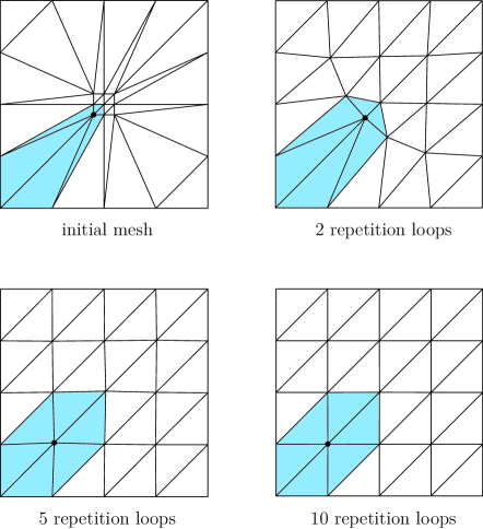
Figure 1: Investigation of the number of repetition loops required to globally improve the mesh. The blue zone indicates the ball of elements sharing the lower left internal node.

In the example, the quality improvement of the ball associated with the lower left internal node (blue zone in Fig. 1) lags behind the other after two iterations. This is a consequence of the current strategy that globally improves the mesh: all balls in the mesh are processed in a fixed order in every repetition loop. It might be more effective to process randomly picked groups of elements, but this has not been implemented yet.

The influence of the smoothing algorithm on mesh grading is investigated in the second example. Graded or anisotropic meshes made up of elements of prescribed size are often present in finite element analysis, e.g. when the computational model contains regions of secondary interest. In these cases it is important to preserve the prescribed element size. Fig. 2a shows a structured triangle mesh zone with constant density interlaced with a coarser structured mesh. The small interface zone is unstructured and contains distorted elements, whereas the structured parts of the mixed mesh are of best quality. An appropriate smoothing algorithm hence would improve the interface zone and would leave the structured zones unchanged.

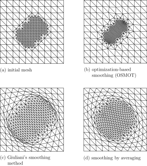
Figure 2: Influence of the smoothing algorithm on mesh grading after 1000 repetition loops.

It can be seen from Fig. 2b that after 1000 global loops running over the internal nodes the optimization-based algorithm (Alg. 3) results in the mesh with the highest quality. Structure is disturbed only slightly and the node density distribution resp. the size of elements is largely preserved. In contrast to that, Giuliani’s method [15] as well as smoothing by weighted averaging [14] fail the test (Fig. 2c and d, respectively). Both heuristic procedures blow up the finer mesh zone, leading to a mesh with equal-sized elements at repeated application. The quality of elements at the interface deteriorated, Giuliani’s method even caused degenerate elements. The tendency to equalize the size of elements is an undesirable feature which arises from the use of averaged geometric measures in the governing equations of the heuristic algorithms.

6.2 Non-convexly distorted mesh

A non-convexly distorted mesh is a mesh that contains stretched and/or skewed elements in the vicinity of the indented boundary, which probably has a high curvature. The automatic regularization of such a mesh at fixed connectivity is very challenging. On the other hand, problems associated with non-convexly distorted meshes constitute important benchmark problems for the implemented smoothing algorithms.

Backward extrusion is a common numerical example where non-convex regions are created when large material deformation occurs. In this initial boundary value problem a billet is loaded into a heavy walled container and then a die is moved towards the billet, so that the material is pushed through the die. Provided that the die and the container are rigid and their surfaces are rough respectively smooth, it suffices to discretize only the billet by finite elements (Fig. 3). Nodes aligned with the lower horizontal boundary are fixed in vertical direction, whereas nodes at the wall of the container are fixed in horizontal direction. The nodes located directly below the die are horizontally fixed and will be displaced in vertical direction to model the die moving downward.

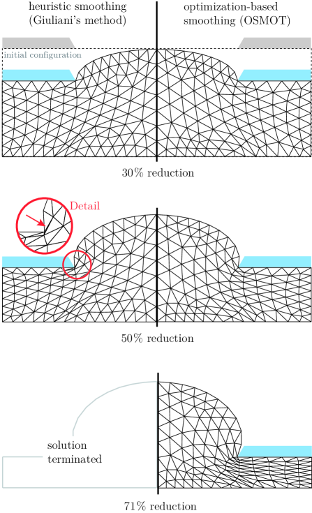
Figure 3: Comparison of an heuristic smoothing method and the developed optimization-based algorithm when applied to the numerical simulation of backward extrusion.

Fig. 3 above shows the edges of the undeformed billet together with the deformed mesh at 30 % height reduction. The left hand side shows the results of the calculation using a heuristic scheme for mesh smoothing. Giuliani’s method [15] for internal meshes has been employed, but smoothing by weighted averaging would yield similar results. The mesh on the right hand side results from the optimization-based smoothing algorithm developed in this paper. In both calculations the simple averaging procedure summarized in Alg. 2 was chosen to smooth the boundary mesh.

The mesh quality of regions immediately under the die is comparable at 30 % height reduction. Near the lower boundary, the optimization-based algorithm produces a slightly smoother mesh. At 50 % reduction, the heavy squeezing of elements around the corner of the die cannot be avoided when using the heuristic method. The area of one element even vanishes, which inhibits convergence of the solution at continued extrusion. Compared to the heuristic method, optimization-based smoothing achieves an excellent mesh regularization. At 50 % height reduction, element squeezing is moderate, even in the non-convexly distorted region at the corner of the die. However, at continued extrusion the fixed mesh connectivity associated with smoothing algorithms limits gains of mesh quality. Calculation terminates at height reductions of more than 71 %. Only a complete remeshing would eliminate degenerate elements so as to continue solution.

6.3 Penetration of a flat-ended pile

The rigorous modeling of penetration is very challenging, especially when the behavior of the penetrated material is highly nonlinear. The final example is concerned with mesh smoothing during the ALE simulation of the penetration of a flat-ended pile into sand. It should be considered as an academic extreme example highlighting the robustness of the new smoothing algorithm when applied to large deformation problems involving indented material boundaries. Details of the ALE method and the constitutive equation used to model the mechanical behavior of sand can be found in [11].

The axisymmetric finite element model is depicted in Fig. 4a. As penetration starts from the ground surface, the initial configuration has a simple geometry. The pile is assumed rigid, its shaft is assumed perfectly smooth, and the pile base is perfectly rough (no sliding). The entire pile skin and the ground surface are modeled as a contact pair using straight segments for the sand surface and accounting for large deformation of the interface. All nodes at the lower boundary of the computational domain are fixed in vertical direction, and the nodes at the vertical boundaries are fixed in radial direction.

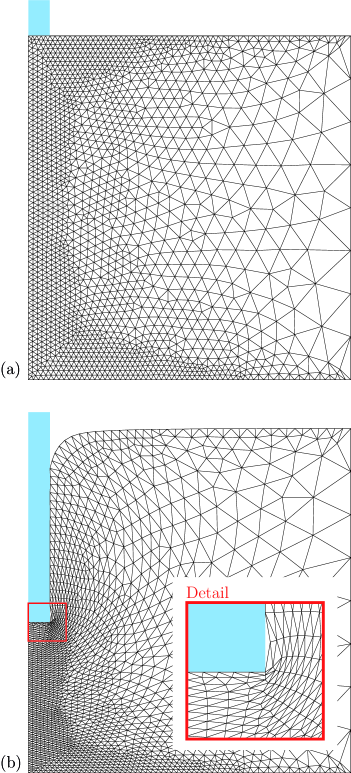
Figure 4: ALE simulation of the penetration of a flat-ended pile using the optimization-based algorithm. (a) Initial mesh, (b) deformed and smoothed mesh at a relative penetration depth of $z/D=4.5$.

For a relative penetration depth of $z/D=4.5$, where $D$ denotes the diameter of the pile, the deformed and smoothed mesh is shown in Fig. 4b. The initially rectangular computational domain is severely deformed by indentation, resulting in a drastic increase of the perimeter-to-area ratio. Elements at the elongated boundary are stretched, i.e. the density of nodes is reduced. On the other hand, the local reduction in height of the domain below the pile base comes along with squeezing of elements. Optimization-based smoothing has indeed improved mesh quality in this example. However, it could not completely avoid element distortion because the mesh topology is fixed, that is, the mesh underneath the pile cannot “get out of the way”. Unless the computational domain would be completely remeshed the numerical model must contain a larger “stockpile” of less deformed mesh in vertical direction in order to achieve a higher mesh quality.

7 Conclusions

Heuristic smoothing algorithms, though they are simple and fast, are inapplicable if the meshed domain becomes non-convex with high curvature. Such situations may occur in initial mesh improvement as well as in numerical simulations of large deformation problems. In order to overcome these problems, an optimization-based smoothing algorithm for triangle meshes has been developed in this paper. The main objective was to continuously rezone the mesh in an arbitrary Lagrangian-Eulerian method for penetration problems [11].

The smoothing algorithm operates iteratively on a local level and distinguishes between boundary nodes and internal nodes. For internal nodes, an optimization procedure has been developed which processes the ball of elements enclosing a common node. It is initiated if the quality measure based on the triangle’s radius ratio drops below a certain value specified by the user. A globally smoothed mesh is pursued by loops repeatedly running over the nodes of elements that fail the quality check. Numerical examples show that the overall procedure, referred to as the OSMOT (Optimization-based SMOothing of Triangle meshes) algorithm, is efficient, extremely robust, and delivers excellent results for both structured and unstructured triangle meshes over arbitrarily shaped (i.e. convex and non-convex) domains.

During penetration, an initially convex computational domain necessarily becomes indented resp. non-convex with high curvature when material boundaries are explicitly resolved by element edges. At drastic changes of the domain’s shape due to large penetration distances mesh quality improvement by smoothing can only be achieved if there is a sufficiently large stockpile of less deformed mesh. This would generally call for numerical models in which the number of finite elements becoming additionally necessary increases disproportionately with the desired penetration distance. In this case, however, it is recommended to completely remesh the computational domain or to try a different modeling technique.

Appendix A Geometric primitives of triangles

Consider a generic element $\triangle\!\subset\mathcal{S}=\mathbb{R}^{2}$ of a plane triangle mesh representing a 2-simplex. The local nodes $0,1,2\in\triangle$ occupy points $\mathbold{x}_{k}=(x_{k},y_{k})^{\mathrm{T}}\in\mathbb{R}^{2}$, with $k\in\{0,1,2\}$. The local connectivity of the generic triangle is predefined by choosing the first node $0$ and then assigning the numbers of the other two nodes $1$ and $2$ in a counter-clockwise manner such that the signed area $A$ given by

$$2A=\det\left(\begin{array}[]{cc}x_{1}-x_{0}&x_{2}-x_{0}\\ y_{1}-y_{0}&y_{2}-y_{0}\\ \end{array}\right)$$ (A1)

is positive. The lengths of the edges are readily available from

$$a\overset{\mathrm{def}}{=}\|\mathbold{x}_{1}-\mathbold{x}_{0}\|\,,\qquad b\overset{\mathrm{def}}{=}\|\mathbold{x}_{2}-\mathbold{x}_{1}\|\,,\qquad\mbox{and}\qquad c\overset{\mathrm{def}}{=}\|\mathbold{x}_{0}-\mathbold{x}_{2}\|\,,$$ (A2)

with $\|\mathbold{x}_{k}-\mathbold{x}_{l}\|=\sqrt{(x_{k}-x_{l})^{2}+(y_{k}-y_{l})^{2}}$ and $k,l\in\{0,1,2\}$. The following relations for triangles are well-known from undergraduate texts in geometry [31]:

semiperimeter: $$s=\tfrac{1}{2}(a+b+c)\,,$$ (A3)

Heron’s formula: $$|A|=\sqrt{s(s-a)(s-b)(s-c)}\,,$$ (A4)

incircle radius: $$r=\dfrac{|A|}{s}\,,$$ (A5)

circumcircle radius: $$R=\dfrac{abc}{4|A|}\,.$$ (A6)

The functional dependence of $s,A,r,$ and $R$ on $(\mathbold{x}_{0},\mathbold{x}_{1},\mathbold{x}_{2})$ is being understood.

Appendix B Gradient and Hessian for mesh optimization

B.1 General remarks

The optimization-based iterative local mesh smoothing algorithm for internal nodes (Alg. 3) requires frequent evaluation of the gradient and Hessian of the element objective function. By assuming that the numbering of the local nodes is in accordance with Section 2.1 and assuming that the locations $\mathbold{x}_{1},\mathbold{x}_{2}$ of the local triangle nodes $1,2\in\triangle$ are constant during the iteration process, the currently implemented objective function for a triangle in the $j$-th iteration takes the form

$$w(\mathbold{x}^{j}_{0})=\frac{R}{R_{\mathrm{ref}}}\left(\frac{R}{r}\right)^{3}=\frac{(abc)^{4}s^{3}}{4^{4}R_{\mathrm{ref}}A^{7}}\;,$$ (B1)

where (A5) and (A6) have been used, and the functional dependence of $a,b,c,s,$ $A,r,R$ on $(\mathbold{x}^{j}_{0},\mathbold{x}_{1},\mathbold{x}_{2})$ is being understood. By dropping the superscribed $j$ indicating the iteration step in what follows, the gradient and Hessian of $w(\mathbold{x}_{0})$ in $\mathbb{R}^{2}$ are the component matrices given by

$$\boldsymbol{\nabla}w(\mathbold{x}_{0})=\left(\begin{array}[]{c}\frac{\partial w}{\partial x_{0}}\\ \frac{\partial w}{\partial y_{0}}\\ \end{array}\right)\qquad\mbox{and}\qquad\mathbold{H}_{\!w}(\mathbold{x}_{0})=\left(\begin{array}[]{ccc}\frac{\partial^{2}w}{\partial x^{2}_{0}}&\frac{\partial^{2}w}{\partial x_{0}\partial y_{0}}\\ \frac{\partial^{2}w}{\partial y_{0}\partial x_{0}}&\frac{\partial^{2}w}{\partial y^{2}_{0}}\\ \end{array}\right)\,,$$ (B2)

respectively. The geometric primitives of triangles provided in A enable the straightforward calculation of the components of $\boldsymbol{\nabla}w(\mathbold{x}_{0})$ and $\mathbold{H}_{\!w}(\mathbold{x}_{0})$, see below. Note that the derivatives of $b=\sqrt{(x_{2}-x_{1})^{2}+(y_{2}-y_{1})^{2}}$ with respect to $\mathbold{x}_{0}$, that is, $\frac{\partial b}{\partial x_{0}},\frac{\partial b}{\partial y_{0}},\frac{\partial^{2}b}{\partial x_{0}\partial y_{0}}$, etc., identically vanish.

B.2 First derivatives of objective function

$$\frac{\partial w}{\partial x_{0}}=\; \frac{1}{4^{4}R_{\mathrm{ref}}}\left(\frac{s^{3}}{A^{7}}\frac{\partial}{\partial x_{0}}(abc)^{4}+\frac{(abc)^{4}}{A^{7}}\frac{\partial}{\partial x_{0}}s^{3}+(abc)^{4}s^{3}\frac{\partial}{\partial x_{0}}A^{-7}\right)$$ (B3)

$$\frac{\partial w}{\partial y_{0}}=\; \frac{1}{4^{4}R_{\mathrm{ref}}}\left(\frac{s^{3}}{A^{7}}\frac{\partial}{\partial y_{0}}(abc)^{4}+\frac{(abc)^{4}}{A^{7}}\frac{\partial}{\partial y_{0}}s^{3}+(abc)^{4}s^{3}\frac{\partial}{\partial y_{0}}A^{-7}\right)$$ (B4)

B.2.1 Extensions

$$\frac{\partial}{\partial x_{0}}(abc)^{4}=\; 4b(abc)^{3}(cC_{1x}+aC_{2x})$$ (B5)

$$\frac{\partial}{\partial y_{0}}(abc)^{4}=\; 4b(abc)^{3}(cC_{1y}+aC_{2y})$$ (B6)

$$\frac{\partial}{\partial x_{0}}s^{3}=\; 3s^{2}C_{3x}$$ (B7)

$$\frac{\partial}{\partial y_{0}}s^{3}=\; 3s^{2}C_{3y}$$ (B8)

$$\frac{\partial}{\partial x_{0}}A^{-7}=\; -\frac{7}{2A^{9}}\big{[}(2s-b)(s-a)(s-c)C_{3x}$$

$$+s(s-b)(s-c)C_{4x}+s(s-a)(s-b)C_{5x}\big{]}$$ (B9)

$$\frac{\partial}{\partial y_{0}}A^{-7}=\; -\frac{7}{2A^{9}}\big{[}(2s-b)(s-a)(s-c)C_{3y}$$

$$+s(s-b)(s-c)C_{4y}+s(s-a)(s-b)C_{5y}\big{]}$$ (B10)

$$\frac{\partial A}{\partial x_{0}}=\; -\frac{A^{8}}{7}\frac{\partial}{\partial x_{0}}A^{-7}$$ (B11)

$$\frac{\partial A}{\partial y_{0}}=\; -\frac{A^{8}}{7}\frac{\partial}{\partial y_{0}}A^{-7}$$ (B12)

B.2.2 Abbreviations

$$C_{1x}\overset{\mathrm{def}}{=}\; \frac{\partial a}{\partial x_{0}}=\frac{\partial}{\partial x_{0}}\left((x_{1}-x_{0})^{2}+(y_{1}-y_{0})^{2}\right)^{\frac{1}{2}}=-\frac{x_{1}-x_{0}}{a}$$ (B13)

$$C_{1y}\overset{\mathrm{def}}{=}\; \frac{\partial a}{\partial y_{0}}=\frac{\partial}{\partial y_{0}}\left((x_{1}-x_{0})^{2}+(y_{1}-y_{0})^{2}\right)^{\frac{1}{2}}=-\frac{y_{1}-y_{0}}{a}$$ (B14)

$$C_{2x}\overset{\mathrm{def}}{=}\; \frac{\partial c}{\partial x_{0}}=\frac{\partial}{\partial x_{0}}\left((x_{0}-x_{2})^{2}+(y_{0}-y_{2})^{2}\right)^{\frac{1}{2}}=\frac{x_{0}-x_{2}}{c}$$ (B15)

$$C_{2y}\overset{\mathrm{def}}{=}\; \frac{\partial c}{\partial y_{0}}=\frac{\partial}{\partial y_{0}}\left((x_{0}-x_{2})^{2}+(y_{0}-y_{2})^{2}\right)^{\frac{1}{2}}=\frac{y_{0}-y_{2}}{c}$$ (B16)

$$C_{3x}\overset{\mathrm{def}}{=}\; \frac{\partial s}{\partial x_{0}}=\frac{1}{2}\left(\frac{\partial a}{\partial x_{0}}+\frac{\partial b}{\partial x_{0}}+\frac{\partial c}{\partial x_{0}}\right)=\frac{1}{2}(C_{1x}+C_{2x})$$ (B17)

$$C_{3y}\overset{\mathrm{def}}{=}\; \frac{\partial s}{\partial y_{0}}=\frac{1}{2}\left(\frac{\partial a}{\partial y_{0}}+\frac{\partial b}{\partial y_{0}}+\frac{\partial c}{\partial y_{0}}\right)=\frac{1}{2}(C_{1y}+C_{2y})$$ (B18)

$$C_{4x}\overset{\mathrm{def}}{=}\; \frac{\partial(s-a)}{\partial x_{0}}=\frac{\partial s}{\partial x_{0}}-\frac{\partial a}{\partial x_{0}}=C_{3x}-C_{1x}$$ (B19)

$$C_{4y}\overset{\mathrm{def}}{=}\; \frac{\partial(s-a)}{\partial y_{0}}=\frac{\partial s}{\partial y_{0}}-\frac{\partial a}{\partial y_{0}}=C_{3y}-C_{1y}$$ (B20)

$$C_{5x}\overset{\mathrm{def}}{=}\; \frac{\partial(s-c)}{\partial x_{0}}=\frac{\partial s}{\partial x_{0}}-\frac{\partial c}{\partial x_{0}}=C_{3x}-C_{2x}$$ (B21)

$$C_{5y}\overset{\mathrm{def}}{=}\; \frac{\partial(s-c)}{\partial y_{0}}=\frac{\partial s}{\partial y_{0}}-\frac{\partial c}{\partial y_{0}}=C_{3y}-C_{2y}$$ (B22)

B.3 Second derivatives of objective function

$$\frac{\partial^{2}w}{\partial x_{0}^{2}}=\; \frac{1}{4^{4}R_{\mathrm{ref}}}\left(\frac{s^{3}}{A^{7}}\frac{\partial^{2}}{\partial x_{0}^{2}}(abc)^{4}+\frac{(abc)^{4}}{A^{7}}\frac{\partial^{2}}{\partial x_{0}^{2}}s^{3}+s^{3}(abc)^{4}\frac{\partial^{2}}{\partial x_{0}^{2}}A^{-7}\right.$$

$$+\frac{2}{A^{7}}\frac{\partial}{\partial x_{0}}(abc)^{4}\frac{\partial}{\partial x_{0}}s^{3}+2s^{3}\frac{\partial}{\partial x_{0}}(abc)^{4}\frac{\partial}{\partial x_{0}}A^{-7}$$

$$\left.+2(abc)^{4}\frac{\partial}{\partial x_{0}}s^{3}\frac{\partial}{\partial x_{0}}A^{-7}\right)$$ (B23)

$$\frac{\partial^{2}w}{\partial y_{0}^{2}}=\; \frac{1}{4^{4}R_{\mathrm{ref}}}\left(\frac{s^{3}}{A^{7}}\frac{\partial^{2}}{\partial y_{0}^{2}}(abc)^{4}+\frac{(abc)^{4}}{A^{7}}\frac{\partial^{2}}{\partial y_{0}^{2}}s^{3}+s^{3}(abc)^{4}\frac{\partial^{2}}{\partial y_{0}^{2}}A^{-7}\right.$$

$$+\frac{2}{A^{7}}\frac{\partial}{\partial y_{0}}(abc)^{4}\frac{\partial}{\partial y_{0}}s^{3}+2s^{3}\frac{\partial}{\partial y_{0}}(abc)^{4}\frac{\partial}{\partial y_{0}}A^{-7}$$

$$\left.+2(abc)^{4}\frac{\partial}{\partial y_{0}}s^{3}\frac{\partial}{\partial y_{0}}A^{-7}\right)$$ (B24)

$$\frac{\partial^{2}w}{\partial x_{0}\partial y_{0}}=\; \frac{1}{4^{4}}\left(\frac{s^{3}}{A^{7}}\frac{\partial^{2}}{\partial x_{0}\partial y_{0}}(abc)^{4}+\frac{1}{A^{7}}\frac{\partial}{\partial x_{0}}(abc)^{4}\frac{\partial}{\partial y_{0}}s^{3}\right.$$

$$+s^{3}\frac{\partial}{\partial x_{0}}(abc)^{4}\frac{\partial}{\partial y_{0}}A^{-7}+\frac{1}{A^{7}}\frac{\partial}{\partial y_{0}}(abc)^{4}\frac{\partial}{\partial x_{0}}s^{3}$$

$$+\frac{(abc)^{4}}{A^{7}}\frac{\partial^{2}}{\partial x_{0}\partial y_{0}}s^{3}+(abc)^{4}\frac{\partial}{\partial x_{0}}s^{3}\frac{\partial}{\partial y_{0}}A^{-7}$$

$$+s^{3}\frac{\partial}{\partial y_{0}}(abc)^{4}\frac{\partial}{\partial x_{0}}A^{-7}+(abc)^{4}\frac{\partial}{\partial y_{0}}s^{3}\frac{\partial}{\partial x_{0}}A^{-7}$$

$$\left.+s^{3}(abc)^{4}\frac{\partial^{2}}{\partial x_{0}\partial y_{0}}A^{-7}\right)=\frac{\partial^{2}w}{\partial y_{0}\partial x_{0}}$$ (B25)

B.3.1 Extensions

$$\frac{\partial^{2}}{\partial^{2}x_{0}}(abc)^{4}=\; 12b(abc)^{2}(cC_{1x}+aC_{2x})^{2}$$

$$+4b(abc)^{3}(cD_{1x}+aD_{2x}+2C_{1x}C_{2x})$$ (B26)

$$\frac{\partial^{2}}{\partial^{2}y_{0}}(abc)^{4}=\; 12b(abc)^{2}(cC_{1y}+aC_{2y})^{2}$$

$$+4b(abc)^{3}(cD_{1y}+aD_{2y}+2C_{1y}C_{2y})$$ (B27)

$$\frac{\partial^{2}}{\partial x_{0}\partial y_{0}}(abc)^{4}=\; 12b(abc)^{2}(cC_{1x}+aC_{2x})(cC_{1y}+aC_{2y})$$

$$+4b(abc)^{3}(cE_{1}+C_{1x}C_{2y}+C_{1y}C_{2x}+aE_{2})$$ (B28)

$$\frac{\partial^{2}}{\partial x_{0}^{2}}s^{3}=\; 6sC_{3x}^{2}+3s^{2}D_{3x}$$ (B29)

$$\frac{\partial^{2}}{\partial y_{0}^{2}}s^{3}=\; 6sC_{3y}^{2}+3s^{2}D_{3y}$$ (B30)

$$\frac{\partial^{2}}{\partial x_{0}\partial y_{0}}s^{3}=\; 6sC_{3x}C_{3y}+3s^{2}E_{3}$$ (B31)

$$\frac{\partial^{2}}{\partial x_{0}^{2}}A^{-7}=\; \frac{63}{A^{9}}\left(\frac{\partial A}{\partial x_{0}}\right)^{2}$$

$$-\frac{7}{2A^{9}}\big{[}(s-a)\{(s-b)(sD_{5x}+(s-c)D_{3x}+2C_{3x}C_{5x})$$

$$+(s-c)(sD_{3x}+2C_{3x}^{2})+2sC_{3x}C_{5x}\}$$

$$+(s-b)\{(s-c)(sD_{4x}+2C_{3x}C_{4x})+2sC_{4x}C_{5x}\}$$

$$+2s(s-c)C_{3x}C_{4x}\big{]}$$ (B32)

$$\frac{\partial^{2}}{\partial y_{0}^{2}}A^{-7}=\; \frac{63}{A^{9}}\left(\frac{\partial A}{\partial y_{0}}\right)^{2}$$

$$-\frac{7}{2A^{9}}\big{[}(s-a)\{(s-b)(sD_{5y}+(s-c)D_{3y}+2C_{3y}C_{5y})$$

$$+(s-c)(sD_{3y}+2C_{3y}^{2})+2sC_{3y}C_{5y}\}$$

$$+(s-b)\{(s-c)(sD_{4y}+2C_{3y}C_{4y})+2sC_{4y}C_{5y}\}$$

$$+2s(s-c)C_{3y}C_{4y}\big{]}$$ (B33)

$$\frac{\partial^{2}}{\partial x_{0}\partial y_{0}}A^{-7}=\; \frac{63}{A^{9}}\frac{\partial A}{\partial y_{0}}\frac{\partial A}{\partial x_{0}}$$

$$-\frac{7}{2A^{9}}\big{[}(s-a)\{(s-b)(C_{3x}C_{5y}\!+\!(s-c)E_{3}+C_{5x}C_{3y}+sE_{5})$$

$$+(s-c)(2C_{3x}C_{3y}+sE_{3})+s(C_{5x}C_{3y}+C_{3x}C_{5y})\}$$

$$+s(s-c)(C_{3x}C_{4y}+C_{4x}C_{3y})+(s-b)\{s(C_{4x}C_{5y}+C_{5x}C_{4y})$$

$$+(s-c)(C_{3x}C_{4y}+C_{4x}C_{3y}+sE_{4})\}\big{]}$$ (B34)

B.3.2 Abbreviations

$$D_{1x}\overset{\mathrm{def}}{=}\; \frac{\partial^{2}a}{\partial x_{0}^{2}}=\frac{\partial}{\partial x_{0}}\left(-\frac{x_{1}-x_{0}}{a}\right)=\frac{x_{1}-x_{0}}{a^{2}}C_{1x}+\frac{1}{a}$$ (B35)

$$D_{1y}\overset{\mathrm{def}}{=}\; \frac{\partial^{2}a}{\partial y_{0}^{2}}=\frac{\partial}{\partial y_{0}}\left(-\frac{y_{1}-y_{0}}{a}\right)=\frac{y_{1}-y_{0}}{a^{2}}C_{1y}+\frac{1}{a}$$ (B36)

$$D_{2x}\overset{\mathrm{def}}{=}\; \frac{\partial^{2}c}{\partial x_{0}^{2}}=-\frac{x_{0}-x_{2}}{c^{2}}C_{2x}+\frac{1}{c}$$ (B37)

$$D_{2y}\overset{\mathrm{def}}{=}\; \frac{\partial^{2}c}{\partial y_{0}^{2}}=-\frac{y_{0}-y_{2}}{c^{2}}C_{2y}+\frac{1}{c}$$ (B38)

$$D_{3x}\overset{\mathrm{def}}{=}\; \frac{\partial^{2}s}{\partial x_{0}^{2}}=\frac{\partial}{\partial x_{0}}\left(\frac{\partial}{\partial x_{0}}\frac{a+b+c}{2}\right)=\frac{1}{2}(D_{1x}+D_{2x})$$ (B39)

$$D_{3y}\overset{\mathrm{def}}{=}\; \frac{\partial^{2}s}{\partial y_{0}^{2}}=\frac{\partial}{\partial y_{0}}\left(\frac{\partial}{\partial y_{0}}\frac{a+b+c}{2}\right)=\frac{1}{2}(D_{1y}+D_{2y})$$ (B40)

$$D_{4x}\overset{\mathrm{def}}{=}\; \frac{\partial^{2}(s-a)}{\partial x_{0}^{2}}=\frac{\partial^{2}s}{\partial x_{0}^{2}}-\frac{\partial^{2}a}{\partial x_{0}^{2}}=D_{3x}-D_{1x}$$ (B41)

$$D_{4y}\overset{\mathrm{def}}{=}\; \frac{\partial^{2}(s-a)}{\partial y_{0}^{2}}=\frac{\partial^{2}s}{\partial y_{0}^{2}}-\frac{\partial^{2}a}{\partial y_{0}^{2}}=D_{3y}-D_{1y}$$ (B42)

$$D_{5x}\overset{\mathrm{def}}{=}\; \frac{\partial^{2}(s-c)}{\partial x_{0}^{2}}=\frac{\partial^{2}s}{\partial x_{0}^{2}}-\frac{\partial^{2}c}{\partial x_{0}^{2}}=D_{3x}-D_{2x}$$ (B43)

$$D_{5y}\overset{\mathrm{def}}{=}\; \frac{\partial^{2}(s-c)}{\partial y_{0}^{2}}=\frac{\partial^{2}s}{\partial y_{0}^{2}}-\frac{\partial^{2}c}{\partial y_{0}^{2}}=D_{3y}-D_{2y}$$ (B44)

$$E_{1}\overset{\mathrm{def}}{=}\; \frac{\partial^{2}a}{\partial x_{0}\partial y_{0}}=-\frac{\partial}{\partial y_{0}}\left(\frac{x_{1}-x_{0}}{a}\right)=-\frac{(x_{1}-x_{0})(y_{1}-y_{0})}{a^{3}}$$ (B45)

$$E_{2}\overset{\mathrm{def}}{=}\; \frac{\partial^{2}c}{\partial x_{0}\partial y_{0}}=\frac{\partial}{\partial y_{0}}\left(\frac{x_{0}-x_{2}}{c}\right)=-\frac{(x_{0}-x_{2})(y_{0}-y_{2})}{c^{3}}$$ (B46)

$$E_{3}\overset{\mathrm{def}}{=}\; \frac{\partial^{2}s}{\partial x_{0}\partial y_{0}}=\frac{1}{2}\left(\frac{\partial^{2}a}{\partial x_{0}\partial y_{0}}+\frac{\partial^{2}b}{\partial x_{0}\partial y_{0}}+\frac{\partial^{2}c}{\partial x_{0}\partial y_{0}}\right)=\frac{1}{2}(E_{1}+E_{2})$$ (B47)

$$E_{4}\overset{\mathrm{def}}{=}\; \frac{\partial^{2}(s-a)}{\partial x_{0}\partial y_{0}}=\frac{\partial^{2}s}{\partial x_{0}\partial y_{0}}-\frac{\partial^{2}a}{\partial x_{0}\partial y_{0}}=E_{3}-E_{1}$$ (B48)

$$E_{5}\overset{\mathrm{def}}{=}\; \frac{\partial^{2}(s-c)}{\partial x_{0}\partial y_{0}}=\frac{\partial^{2}s}{\partial x_{0}\partial y_{0}}-\frac{\partial^{2}c}{\partial x_{0}\partial y_{0}}=E_{3}-E_{2}$$ (B49)

References

• [1] A. Liu and B. Joe. Relationship between tetrahedron shape measures. BIT, 34:268–287, 1994.
• [2] D. A. Field. Qualitative measures for initial meshes. International Journal for Numerical Methods in Engineering, 47:887–906, 2000.
• [3] P. M. Knupp. Algebraic mesh quality metrics. SIAM Journal on Scientific Computing, 23(1):193–218, 2001.
• [4] P. J. Frey and P.-L. George. Mesh Generation: Application to Finite Elements. HERMES Science Europe Ltd., Oxford, UK, 2000.
• [5] C. W. Hirt, A. A. Amsden, and J. L. Cook. An arbitrary Lagrangian-Eulerian computing method for all flow speeds. Journal of Computational Physics, 14:227–253, 1974.
• [6] T. J. R. Hughes, W. K. Liu, and T. K. Zimmermann. Lagrangian-Eulerian finite element formulation for incompressible viscous flows. Computer Methods in Applied Mechanics and Engineering, 29:329–349, 1981.
• [7] D. J. Benson. An efficient, accurate, simple ALE method for nonlinear finite element programs. Computer Methods in Applied Mechanics and Engineering, 72(3):305–350, 1989.
• [8] M. Nazem, D. Sheng, J. P. Carter, and S. W. Sloan. Arbitrary Lagrangian-Eulerian method for large-strain consolidation problems. International Journal for Numerical and Analytical Methods in Geomechanics, 32(9):1023–1050, 2008.
• [9] S. A. Savidis, D. Aubram, and F. Rackwitz. Arbitrary Lagrangian-Eulerian finite element formulation for geotechnical construction processes. Journal of Theoretical and Applied Mechanics, 38(1-2):165–194, 2008.
• [10] D. Aubram, F. Rackwitz, and S. A. Savidis. An ALE finite element method for cohesionless soil at large strains: Computational aspects and applications. In T. Benz and S. Nordal, editors, Proceedings 7th European Conference on Numerical Methods in Geotechnical Engineering (NUMGE 2010), pages 245–250. CRC Press, London, 2010.
• [11] D. Aubram. An Arbitrary Lagrangian-Eulerian Method for Penetration into Sand at Finite Deformation. Number 62 in Veröffentlichungen des Grundbauinstitutes der Technischen Universität Berlin. Shaker Verlag, Aachen, 2013. http://opus4.kobv.de/opus4-tuberlin/frontdoor/index/index/docId/4755.
• [12] D. J. Benson. Computational methods in Lagrangian and Eulerian hydrocodes. Computer Methods in Applied Mechanics and Engineering, 99(2-3):235–394, 1992.
• [13] J. Donea, A. Huerta, J.-Ph. Ponthot, and A. Rodríguez-Ferran. Arbitrary Lagrangian-Eulerian Methods, volume 1 of Encyclopedia of Computational Mechanics, chapter 14. John Wiley & Sons, Ltd., 2004.
• [14] J. L. F. Aymone, E. Bittencourt, and G. J. Creus. Simulation of 3d metal-forming using an arbitrary Lagrangian-Eulerian finite element method. Journal of Materials Processing Technology, 110:218–232, 2001.
• [15] S. Giuliani. An algorithm for continuous rezoning of the hydrodynamic grid in arbitrary Lagrangian-Eulerian computer codes. Nuclear Engineering and Design, 72:205–212, 1982.
• [16] R. Löhner, K. Morgan, and O. C. Zienkiewicz. Adaptive grid refinement for the compressible Euler equations. In I. Babuška, O. C. Zienkiewicz, J. Gago, and E. R. A. Oliviera, editors, Accuracy Estimates and Adaptive Refinements in Finite Element Computations, pages 281–297. John Wiley & Sons, Ltd., 1986.
• [17] W. D. Barfield. An optimal mesh generator for Lagrangian hydrodynamic calculations in two space dimensions. Journal of Computational Physics, 6:417–429, 1970.
• [18] J. U. Brackbill and J. S. Saltzman. Adaptive zoning for singular problems in two dimensions. Journal of Computational Physics, 46:342–368, 1982.
• [19] S. R. Kennon and G. S. Dulikravich. Generation of computational grids using optimization. AIAA Journal, 24(7):1069–1073, 1986.
• [20] E. A. Dari and G. C. Buscaglia. Mesh optimization: How to obtain good unstructured 3d finite element meshes with not-so-good mesh generators. Structural and Multidisciplinary Optimization, 8:181–188, 1993.
• [21] P. D. Zavattieri, E. A. Dari, and G. C. Buscaglia. Optimization strategies in unstructured mesh generation. International Journal for Numerical Methods in Engineering, 39:2055–2071, 1996.
• [22] M. S. Joun and M. C. Lee. Quadrilateral finite-element generation and mesh quality control for metal forming simulation. International Journal for Numerical Methods in Engineering, 40:4059–4075, 1997.
• [23] H. Braess and P. Wriggers. Arbitrary Lagrangian Eulerian finite element analysis of free surface flow. Computer Methods in Applied Mechanics and Engineering, 190:95–109, 2000.
• [24] P. M. Knupp, L. G. Margolin, and M. Shashkov. Reference Jacobian optimization-based rezone strategies for arbitrary Lagrangian Eulerian methods. Journal of Computational Physics, 176:93–128, 2002.
• [25] V. Dyadechko, R. Garimella, and M. Shashkov. Reference Jacobian rezoning strategy for arbitrary Lagrangian-Eulerian methods on polyhedral grids. Report LA-UR-05-8159, Los Alamos National Laboratory, Los Alamos, USA, 2005.
• [26] W. Sun and Y.-X. Yuan. Optimization Theory and Methods - Nonlinear Programming. Springer Science+Business Media, LLC, 2006.
• [27] D. G. Luenberger and Y. Ye. Linear and Nonlinear Programming. Springer Science+Business Media, LLC, 3rd edition, 2008.
• [28] A. A. Goldstein and J. F. Price. An effective algorithm for minimization. Numerische Mathematik, 10:184–189, 1967.
• [29] L. Armijo. Minimization of functions having Lipschitz continuous first partial derivatives. Computational Mechanics, 16:1–3, 1966.
• [30] P. L. George, H. Borouchaki, P. J. Frey, P. Laug, and E. Saltel. Mesh Generation and Mesh Adaptivity: Theory and Techniques, volume 1 of Encyclopedia of Computational Mechanics, chapter 17. John Wiley & Sons, Ltd., 2004.
• [31] I. N. Bronstein, K. A. Semendjajew, G. Musiol, and H. Mühlig. Handbook of Mathematics. Springer-Verlag Berlin Heidelberg, 5th edition, 2007.